Directional-Sensor Network Deployment Planning for Mobile-Target Search

Abstract

In this paper, a novel time-phased directional-sensor network deployment strategy is presented for the mobile-target search problem, e.g., wilderness search and rescue (WiSAR). The proposed strategy uses probabilistic target-motion models combined with a variation of a standard direct search algorithm to plan the optimal locations of directional-sensors which maximize the likelihood of target detection. A linear sensing model is employed as a simplification for directional-sensor network deployment planning, while considering physical constraints, such as on-time sensor deliverability. Extensive statistical simulations validated our method. One such illustrative experiment is included herein to demonstrate the method’s operation. A comparative study was also carried out, whose summary is included in this paper, to highlight the tangible improvement of our approach versus three traditional deployment strategies: a uniform, a random, and a ring-of-fire type deployment, respectively.

1. Introduction

Wireless sensor networks (WSNs) have been used to effectively monitor various physical phenomena in real-time, where they collect, transmit, and process information in an on-line manner [1]. Their applications include environmental monitoring, [2,3,4,5,6], border security [7], target tracking and localization [8,9,10], urban search and rescue (USAR) [11,12] and lost person detection in wilderness search and rescue (WiSAR) [13,14]. Research in the field, however, often assumes omni-directional sensing models for network-topography planning. This assumption may not hold true for many sensor types, such as video or infrared, which have a directional sensing range [15].

WSNs that utilize directional sensors are, typically, referred to as directional sensor networks (DSNs). In DSNs, a sensor’s sensing model is characterized by a limited angular range in addition to a distal range. Thus, in 2D space, the sensing area of a directional sensor is often modelled as a circular (partial) sector. This contrasts with the sensing area of an omnidirectional sensor, which is a (complete) disk, which is formed when the angular range of a directional sensor is very wide.

Another class of sensing model exists at the other extreme of the spectrum, when the angular range is very small. These are referred to as linear sensing models and represent sensors that have a sensing area that has been constrained to a line, such as a laser [16]. Being a simpler representation of a sensing region, it is typically (computationally) easier to plan the deployment of directional sensors using a linear sensing model. We postulate that the deployment of a directional sensor can be sufficiently approximated by a linear sensing model during deployment planning, with minimal loss in performance, for the problem considered herein.

Determining locations of directional sensors (i.e., positions and orientations—poses) is an important aspect of DSN deployment planning. Pertinent strategies are predominantly formulated with the goal of maximizing some form of coverage. Two common metrics are total area coverage (with minimum holes) (e.g., [17,18,19,20,21,22]) and preferential target coverage (e.g., [23,24,25,26,27]). These objectives are often coupled with secondary objectives such as ensuring connectivity or increasing energy efficiency.

In [18], for example, a tessellation-based approach was used to deploy directional sensors for maximum area coverage. The sensing model is simplified by altering the curved portions of the sector into discretized line segments, forming a hexagonal approximation to the sector. The sensors are then tiled (i.e., placed side by side) into a rectangular deployment area containing polygonal obstacles until either all the sensors are deployed, or the area is fully covered. Coverage holes that naturally develop around obstacles, as a result of the tiling method, are removed by placing auxiliary sensors, which overlap previously deployed sensors.

In [26], directional sensors are deployed to maximize coverage of a number of static target positions (point targets) within a region of interest (RoI). The proposed algorithm is a heuristic that deploys sensors in a sequential manner. The approach starts by determining the distances between the target positions. The coordinates of the target position with the highest number of neighbors is chosen as the optimal sensor position. The orientation of the sensor, placed at these coordinates, is determined by performing a 360° rotation and finding the angle at which the greatest number of neighboring positions are covered. Subsequent sensor poses are determined following the same greedy process.

A substantial area of research within the sensor network literature considers distributed area coverage and coverage control problems. This involves the reconfiguration of mobile sensor networks to maximize total area coverage [28,29,30,31,32,33,34]. This is, typically, performed in bounded regions with resources that can cover a substantial portion of the RoI. However, there are key differences between past research in this area and our work. Mainly, the problem addressed in this paper is not one of maximizing total area coverage: our objective is to maximize the likelihood of detecting a mobile target within an unbounded and growing RoI. The expanding nature of the search implies that one would always have an insufficient number of sensors to cover an appreciable fraction of the search area (i.e., the sensor network only provides sparse coverage). Namely, in our work, it is assumed that the growing search area is significantly larger than the one that can be covered by the available search resources. Achieving non-redundant coverage, where no sensors overlap is, therefore, a given in the scenario considered, and a reconfiguration to maximize total area coverage would not be necessary. Coverage control research also attempts to maximize area coverage using dynamic density functions. The focus of research in this area has been on motion coordination algorithms of mobile robots to optimize for a generalized time-varying density metric; often, with the use of Voronoi tessellations [35,36,37,38]. Although the density functions considered could represent target motion, as in our work, their solutions are not applicable as they typically assume mobile sensors, in contrast to our static sensors (i.e., sensors that cannot be relocated or reoriented once deployed).

As abovementioned, this paper considers the mobile-target search problem, which has been addressed in the literature using a variety of solutions via sensor networks and robotic UAVs/UGVs. Some solutions rely solely on static sensors [39,40]. However, these often do not consider dynamic scenarios where the target-location likelihood function can change over time, nor do they consider an expanding search area. A modified approach, that deals with these issues, is presented in [41] where a static-sensor network is deployed in a time-phased manner allowing for re-planning if new information on the target were to become available. Others consider only mobile search resources [42,43,44]. Although mobile robots (e.g., UGVs) enable the reconfigurability of the network, they are also expensive to deploy and operate as search resources. In contrast, static sensors can be deployed in greater numbers due to their simplicity and low cost. Hybrid approaches have also been considered where a combination of static and mobile search resources are deployed [45,46]. For example, in [46], mobile robots are used to relocate redundant static sensors to locations of coverage holes. The aforementioned target search literature, typically, employs search resources that are either mobile or have omnidirectional sensing models. In contrast, in this paper, we use homogenous static-directional sensors which, to the best of our knowledge, have not been used to address the mobile target search problem.

Several studies have also been conducted in information-acquisition methods during search and rescue operations utilizing Simultaneous Localization and Mapping (SLAM) [47,48,49]. The objective of these problems is to develop path-planning algorithms for mobile robots to enable them to gather information in complex environments; this information can, then, be used to aid in the search. In contrast, our work, assumes information about the environment is, primarily, an a priori known (e.g., locations of obstacles), which enables us to narrow the focus of our work to topology planning for target detection. Thus, SLAM is considered outside of the scope of this paper.

In other pertinent research works, for example, on target tracking [16,50,51,52], the objective is to obtain an accurate estimate of the target trajectory using positional updates provided by sensor measurements. Solutions to this problem, however, are not directly applicable to target detection since they assume that the target’s initial position is an a priori known, which is not the case during target detection. In barrier coverage [53,54,55,56], the problems addressed are a subset of the preferential coverage problem, where sensors are deployed to create a barrier between two RoIs. However, these, typically, consider sensor deployment within a bounded RoI.

Another important consideration, in sensor network deployment planning, is determining the feasibility of the deployment plan. This ensures that the planned network can be realized by the available delivery resources (e.g., robotic unmanned ground vehicles—UGVs). There has been some research considering sensor delivery during deployment planning [14,45,57,58,59,60,61,62,63,64,65,66]. Typically, these determine optimal robot trajectories, for sensor delivery, according to a pre-determined optimal sensor network plan [45,58,59,60,61,65,66,67]. Our earlier work has considered the optimization of a sensor network constrained to the trajectories of mobile search robots, within a WiSAR context [14]. In contrast, herein, instead of sensors being deployed along pre-defined trajectories, the sensors can be deployed at any pose provided such deliveries meet the time constraints. Thus, we incorporate sensor-delivery time considerations directly into our planning algorithm, which has a direct impact on the poses of the optimal/final network topology.

This paper, thus, considers the problem of deployment planning of sparse DSNs that comprise only static sensors, with the goal of maximizing the probability of detecting a mobile-target in a time-expanding RoI. While our own and others’ earlier works have addressed the mobile-target detection problem using dynamically deployed sensor networks, these have only been for omnidirectional sensors, [41,68,69,70,71]. As this work considers directional sensors, a new solution approach is required. For example, part of the proposed methodology contains an orientation optimization which has not been considered in past works with omnidirectional sensors. Similarly, various aspects of our solution approach are tailored to the directional sensing model type.

In the proposed methodology, sensor deployment poses and times are determined, in order of priority, to maximize the number of simulated target trajectories the sensors would cover, and be feasible for a set of delivery resources, while being adaptable if new information is found. Our work is novel in that it provides a solution method to the maximum intersection problem. This is an uncommon geometric problem where the objective is to place a line, within a plane, to maximize the number of intersections it has with a set of pre-existing lines. In the context of our work, this corresponds to planning the deployment of a sensor (representing the additional line) to maximize the number of simulated target trajectories it would intercept (which represent the pre-existing lines).

Our work is also novel in that it provides a novel sensor-delivery method that incorporates delivery-time constraints directly into the sensor-pose optimization to guarantee sensor network deliverability. Specifically, sensor deployment positions and orientations are planned taking into account when they could be delivered to the deployment location, given the sensor deployment plan thus far. This is an approach that, to the best of our knowledge, has not been addressed in the static-sensor delivery literature.

2. Problem Definition and Background

The problem addressed in this paper is one of localizing a mobile, un-trackable target in an unbounded and growing region (e.g., a person lost in the wilderness). Our focus is on the use of directional static-sensor networks, where the term ‘static’ refers to both the (self) immobility of the sensors as well as our inability to relocate them once deployed. A further constraint is that these static sensors have to be deployed by a set of delivery robots (e.g., robotic UGVs), which, typically, move at a maximum and constant speed. These mobile robots are assumed to have no sensing capabilities and, thus, do not take a direct part in the search. Namely, the set of available resources for the search are categorized as static-directional sensors and robotic delivery UGVs.

2.1. Example Application: Wilderness Search and Rescue (WiSAR)

WiSAR is often time-critical, where available search resources would be insufficient to provide a complete (hole-less) distributed coverage; especially, considering that the search area grows with time. As a result, the effectiveness of individual deployed sensors diminishes with time.

A wilderness search, typically, begins with the notification of a missing person (the target); subsequently, information regarding their last known position (LKP), time at which they were present at this position, and information regarding the target’s demographics is obtained. The target’s travel since leaving the LKP remains unknown, thus, a probabilistic model of his/her motion through the RoI is required. This model could be derived from the statistical behavior of the overall demographic group to which the target belongs [72]. Given an estimate of possible motions that the target could follow, an effective sensor deployment for detecting the target can, then, be planned.

This work assumes that there exists a parallel search effort for the target by mobile operatives. It is anticipated that these operatives would provide feedback to the central search controller in real-time for a potential re-planning of the network deployment (e.g., discovering a clue left by the target). Furthermore, we assume the sensors remain operational for the full duration of the search.

2.2. Line Approximation of a Directional-Sensor

The approximation to a linear sensing model can be determined using the mathematical parameters describing a directional sensor. Geometrically, a directional sensor can be modelled by a 4-tuple (P, θ, R_s, α) [15]: P is the (x, y) position of the node, θ is its working orientation, R_s is its sensing range, and α is the angular sensing range, Figure 1a. Our simplified linear sensing model, herein, is modelled using the same mathematical parameters as those of the directional sensor. The difference is that the angular range is set to α = 0. As a result, it resembles a line segment as shown in Figure 1b.

This simplified model is only used to reduce the computational complexity of our planning algorithm. The final solution for the optimal positions and orientations of the linear sensing model is used to construct the directional sensors. The network performance is, then, evaluated with these directional sensors. Herein, the directional sensors that are constructed from a linear sensor plan are referred to as linear-directional sensors.

2.3. Sensor Plan Performance Measure

The objective of our DSN planning is to determine sensor deployments that maximize the probability of detecting the mobile target. Herein, a sensor network deployment plan, D_s, for a set of n sensors, comprises the sensor positions, {(x₁, y₁), …, (x_n, y_n)}, orientations, {θ₁, …, θ_n)} and corresponding placement times, {t₁, …, t_n)}. The optimization problem at hand can, then, be formulated as:

$${\mathrm{maximize} P (S = \mathrm{success}|\mathit{D}}_s),$$

(1)

where S is a binary random variable denoting the success/failure of a search mission (i.e., a successful target detection).

One may note that it is, typically, not feasible to determine the search success probability exactly. Thus, herein, an estimator of the success probability is used as the objective function. It is defined as the proportion of equally feasible target motions that would be detected by a search:

$${P(S = \mathrm{success}|\mathit{D}}_s) \approx \frac{n_{td}}{n_t},$$

(2)

where n_t is the number of equally likely potential target trajectories, and n_td is the number of targets, on their respective trajectories, that would be detected by a sensor in the deployed DSN. Assuming a linear sensing model, Figure 1b, a moving target would be detected when its trajectory crosses a sensor’s sensing range. In our proposed method, the set of n_t trajectories is simulated using the lost target’s demographics. These trajectories represent a statistical sample of all possible trajectories that the target could have taken from the LKP. Thus, the objective of our sensor-network planning is to maximize the number of these simulated trajectories that would be intercepted by the sensor network (i.e., maximizing n_td). Namely, the planned network maximizes the likelihood of a successful target detection as defined by the abovementioned estimator.

2.4. Optimization Metric for Sensor Planning

The simulated target trajectories are also used to plan the sensor deployment poses within our proposed methodology. In our previous work, such target trajectories were used to inform our deployment planning by defining a target location likelihood function to estimate where the target may be at any given time, t, via a density estimate [68]. The simulated trajectories were also used to define iso-probability curves denoting the limits of where a given percentile target could travel up to in all directions [14]. However, herein, we maximize the cumulative number of trajectories intersected by the sensor network directly. A function, f, that describes the number of simulated trajectories intersected by a directional sensor, of a particular sensing range, R_s, if placed in a certain position, (x,y) at time t, and in an orientation θ, can be defined as,

$$n_i=f\left(x_i,y_i,t_i,{\theta }_i,R_s\right),$$

(3)

where n_i is the scalar value representing the number of trajectories intersected by Sensor i at Position (x_i, y_i) and Orientation θ_i, at Time t_i. As the probability of success, defined in Equations (1) and (2), is determined by the number of targets detected, maximizing the number of trajectories intersected, when planning each sensor pose, also maximizes the estimate of the cumulative probability of success. Thus, f can be set as the objective function which needs to be maximized. This is described by

$$N_i=\max \left\{f\left(x_i,y_i,t_i,{\theta }_i,R_s\right)\right\},$$

(4)

where N_i is the number of trajectories intersected at the optimal position, orientation and time for a particular sensor, i. It should be noted that a distinction is made between the set of simulated trajectories used to plan the sensor deployment and the trajectories used to evaluate the sensor network plan_. Specifically, one set of simulated trajectories, n, was used to plan the poses of the sensors and a separate set of trajectories, n_t, was used to test the performance of the final sensor network plan.

3. Proposed Deployment Methodology

The proposed deployment methodology is a three-phase adaptive approach. First, the strategy determines the (original) deployment poses and times for the sensors at hand, prior to the start of the search (i.e., t_start), in an off-line manner. Next, the original deployment plan is initiated where sensors are deployed at their planned poses, at their corresponding deployment times, by their assigned delivery robots. If during this phase, new information becomes available (e.g., a clue is found), then, the third phase of the proposed strategy is invoked, where the deployment poses and times for the remaining (undeployed) sensors are re-optimized. Since the three phases of the methodology are sequential in nature, they are designed to run on commercially available computing devices and can be assumed to run as a finite-state machine. However, a more helpful model for performance and property analysis may be a random-access stored-program (RASP) machine model of computation. Thus, we assume that our algorithm is not limited by the memory available in modern computers.

3.1. Phase 1: Original Network Planning

The off-line planning process is outlined in Figure 2 and detailed in the following sub-sections.

The proposed methodology plans the placement of directional sensors assuming a linear sensing model in an iterative and sequential manner (i.e., one at a time). In this method, the linear sensing model is used as a simplification of the directional sensing model to reduce the computational complexity of our problem and improve computational efficiency. The proposed methodology commences by simulating a set of possible target trajectories, starting from the LKP, Step 1.1. Next, the best possible sub-region, within the RoI, to place a sensor is determined, Step 1.2. Sensor pose optimization is, then, conducted within the optimal sub-region to determine the optimal planned pose, Step 1.3. The process is repeated until all sensor deployment poses and times are determined. Pseudocode for the overall planning methodology, as described in Figure 2, is included in Appendix A.

3.1.1. Step 1.1: Target Trajectory Generation

There exists extensive literature on developing complex probabilistic motion models to predict the behavior of a lost person based on their demographics and environmental features [73]. However, for simplicity, in this work we simulate the target’s possible motion patterns as randomly generated piecewise linear target trajectories that begin from the target’s LKP [68]. These trajectories represent a statistical sample of all the possible trajectories that the actual target could have taken from the LKP and are used to inform our deployment planning.

The simulated trajectories follow an outward propagation model with a target’s potential proclivity to randomly wander factored in. This is characterized by straight-line segments with probabilistic heading changes. The likelihood of a target walking on a particular heading, θ_t, and travelling a distance along that heading, r, in its motion, is given by:

$$P\left(r\right)=U\left(0,d_m\right),$$

(5)

$$P\left({\theta }_t\right)=N\left(\varphi ,{\sigma }_{\theta }^2\right),$$

(6)

where d_m is the maximum distance the target will walk along a heading, σ_θ is the degree to which the target wanders, and ϕ is the heading directly away from the LKP. A normal distribution centered on the direction directly away from the LKP is used to model target heading changes. The outward propagation model is used since historical data suggests that targets continue travelling in their initial direction of motion after leaving the LKP. The velocity of the targets is modelled as a normal distribution centered on the mean target speed v_mean and standard deviation v_std. Detailed pseudocode describing the implementation of the statistical models to create the simulated target trajectories is given in Appendix B.

In the case of multiple targets, for example, Target A, B, C, etc., separate sets of, n_A, n_B, n_C, etc., trajectories would be simulated for each target based on their respective demographics, and their respective LKPs, respectively. The combined set of trajectories would then be used to inform the deployment planning.

Since deployment execution cannot start at the exact moment of notification of a lost target, a specific deployment start time, t_start, from which sensors can start to be deployed is determined by the search commander. Furthermore, as the search cannot continue indefinitely, an end of search time t_end is also defined. As a result, only the portions of the trajectories that occur between t_start and t_end are considered to inform the deployment planning. Figure 3a below shows a set of 100 target trajectories that start at the LKP (0, 0) at t = 0, and move outward randomly until an end of search time of t_end = 7200 s. Figure 3b shows a set of 100 trajectories with a t_end time of 7200 s and with the portions of the trajectory before the t_start time of 3600 s removed. Thus, the search time duration is defined a priori as [t_start, t_end].

3.1.2. Step 1.2: Deployment Sub-Region and Time Determination

An estimate of the number of trajectories that can be intersected in any region can be determined by examining the density of trajectories in that region. The higher the density, the greater the potential of maximizing the cumulative total of simulated trajectory intersections. In our previous work, a non-uniform polar grid-based approach was used for density prediction [50]. However, this method is not suitable to the maximum intersection problem considered here since it only determines the density of trajectories in locally defined areas within the RoI. A global search is required to determine the sub-region with the highest density of trajectories. Thus, herein, a hierarchical multi-resolution variation of pattern-search optimization is proposed [74]. A similar hierarchical direct search approach, but using a genetic algorithm, can be found in [75]. The proposed pattern search optimization determines a sub-region, within the entire search RoI, that contains the highest density of simulated trajectories so that if a sensor was placed within this sub-region it would intersect the maximum number of trajectories possible.

Our strategy uses a hexagonal pattern, shown as the seven black ×s of the pattern search tool in Figure 4. The sub-region corresponding to each point is shown as a circle, whose size is dependent on the pattern size such that a hole-less coverage is achieved. The objective function evaluated for each iteration of the pattern is the number of trajectories that pass within each of the seven circles centered at the crosses (i.e., the density of trajectories within the circular sub-regions). If the circle, in the center of the stencil, contains the highest density of trajectories, then, the size of the stencil is isometrically reduced. A scale factor of 0.75 was selected to ensure the reconfigured stencil fits within the central sub-region, with no coverage holes. If the highest density is found within one of the outer circles, then, the stencil is translated so that the circle that contained the highest density of trajectories is at the center. The density of trajectories, in the new pattern configuration, is, then, evaluated. This process is repeated until the diameter of the circles is the equivalent length of the defined sensing range. Namely, the pattern search stencil is translated and resized until the sub-region with the highest density of trajectories is found. That sub-region (i.e., the one containing the highest density of trajectories), in the pattern’s final configuration, is selected as the final optimal sub-region within which the sensor is deployed.

The proposed pattern, in its initial, final and two intermediary configurations, is shown in Figure 4, overlaid above a set of 100 target trajectories. It should be noted that only four steps of the pattern search process are shown, in Figure 4, for brevity. Using a circular sub-region, with a final configuration diameter that is the same size as the linear sensing range, allows for a more effective orientation optimization (in the subsequent step), compared to the polar grid approach in our previous work [68], as the sensor line can be swept circularly until an optimal orientation, θ, is found. This design was inspired by the patterns seen in sensor network deployment problems involving k-coverage, where multiple omnidirectional sensors overlap to ensure every point in the RoI is covered by at least k sensors [76,77,78].

Deployment time is incorporated into the pattern search optimization. For each sub-region in the hexagonal pattern, a corresponding deployment time is determined by calculating the earliest time at which a robot could deliver there, based on each robot’s relative distance and previous delivery assignments. Namely, the deployment time of a sensor, at a given location, is calculated by adding the time it would take for a robot to get to the deployment position (i.e., the center of the deployment sub-region) to the time at which the robot was at its previous deployment position.

Figure 5 shows the positions and times, of three delivery robots, at their previous deployment positions as well as the next potential deployment position (black ×). This deployment position represents the center of a deployment sub-region. The distances to the potential position are 2820 m, 1084 m, 580 m for Robots 1, 2, and 3, respectively. For a robot speed of 10 m/s, the earliest deployment times, then, are 4008 s, 3879 s, and 3799 s, respectively. Thus, in this example, the earliest deployment time which could be achieved, by Robot 3, is t₃ = 3799 s. It should be noted that the distance of the delivery robot, from the deployment sub-region, is calculated using the position of the center of the sub-region. However, the sensor is actually positioned on the circumference of the sub-region in the following step of our methodology. This assumption is made as the sensing range (i.e., the diameter of the sub-region) is small enough, in the final configuration, to not have a significant effect on the actual deployment time achieved by the robot.

Once the earliest possible deployment time is determined for each sub-region, only the parts of the simulated target trajectories that occur after the sensor becomes active (i.e., when it is deployed) are considered. Namely, the density of trajectories, for each sub-region, would then be the total number of trajectories that pass through it after its corresponding deployment time. This has a direct effect on the choice of the optimal sub-region as earlier deployment times would result in more trajectory presence in each respective sub-region. The optimal deployment sub-region, at each iteration, is the one that contains the highest number of trajectories. If, however, there are no trajectories present within a sub-region, after the determined deployment time, then a deployment in that sub-region is considered infeasible. Namely, the robot would not be able to deliver in time to intercept any of the trajectories passing through that sub-region. It should be noted that this, typically, only occurs in the initial iterations of the pattern search, due to the large distances of the outer sub-regions from the LKP. In the case that none of the circular sub-regions contain any trajectories, the pattern search algorithm is reinitialized at a position closer to the robots. The process is repeated until a feasible sub-region and corresponding deployment time is found. Detailed pseudocode of the pattern search algorithm is given in Appendix C.

3.1.3. Step 1.3: Sensor Pose Determination

In the previous step, only the density of trajectories that pass through the optimal sub-region was determined. In order to maximize the exact number of trajectories that the sensor would intersect, an orientation optimization is conducted on the simulated trajectories within the optimal sub-region. These simulated trajectories can also be represented as multi-segmented lines. A target would be intercepted, then, if one of the multi-segmented lines, belonging to a particular trajectory, intersects the sensing area of the sensor.

The linear sensor is positioned, within the optimal sub-region, such that its sensing line bisects the circular sub-region. Namely, it is positioned on the circumference of the circular sub-region determined in Step 1.2 and oriented to point towards the center of the region. An example of this is shown in Figure 6 for three sensor orientations spaced by 60°.

The optimal orientation, namely, the one that intersects the greatest number of trajectories, is determined using a simple search engine that is implemented practically using the fminsearch function from MATLAB’s optimization toolbox [79]. As the number of target trajectories intersected by a sensor is a discrete function, the optimization is initialized at several different orientations to avoid converging to a local maximum. Practically, whether or not an intersection exists is determined by equating the linear geometric equations of the line-segment representing the sensor (i.e., the linear sensing model) and the multiple line-segments representing each trajectory. Namely, if a trajectory is to be intersected by a sensor, at least one of the multiple segments of a single trajectory must contain an intersection point with the line representing the sensor. Mathematically, this can be solved using the equations of a pair of line segments [80]. One line is connected between points p₁ and p₂ and the other is connected between points p₃ and p₄. This is described by the following equations:

$$p_i=p_1+t_a\left(p_2-p_1\right),$$

(7)

$$p_i=p_3+t_b\left(p_4-p_3\right),$$

(8)

where p_i is the point of intersection of the two lines and t_a and t_b are the offsets of the intersection point for each corresponding line. In the context of this paper, p₁ and p₂ represent the end points of a particular segment of a trajectory and p₃ and p₄ represent the start and end points of the sensor line, respectively. By equating the two and solving the system of linear equations, values for t_a and t_b can be obtained. If both values satisfy the inequalities,

$$\begin{gathered} 0\le t_a\le 1, \\ 0\le t_b\le 1, \end{gathered}$$

then, a point of intersection exists between the two-line segments. The exact coordinates of the intersection can be found by substituting the values of t_a and t_b back into either Equations (7) or (8), respectively. The pseudocode for the orientation optimization process is included in Appendix D.

The set of trajectories that are intersected, in between each pose determination, are removed and resampled to ensure the same level of information is used to plan subsequent poses. For example, after the pose is determined for Sensor A, the simulated trajectories n_a that were intersected by this sensor, out of the total trajectories n, are removed and re-simulated. The new set of simulated trajectories, which consists of the previously non-intersected trajectories and the re-simulated trajectories, would, then, be used to plan the pose of Sensor B. This approach has to be taken to avoid the depletion of target trajectory information and was inspired by the resampling process of a particle filter [81]. This iterative algorithm is followed until all poses have been planned for all the available sensors. The pseudocode for the trajectory re-simulation process is included in Appendix E.

Once the optimal sensor poses, which were planned using the linear sensing model, are determined, they are subsequently converted to the required directional sensors. Namely, the sensor position (x,y), orientation (θ) and sensing range (R_s) of the linear sensing model are combined with the directional sensing angle, α, to form the DSN. This is reflected, visually, in a change from sensors resembling line-segments (Figure 7a) to those resembling sectors (Figure 7b). The linear-directional sensors (directional sensors that are planned using a linear sensing model) are, subsequently, used to test the performance of the network.

Deployment Example:

An example DSN deployment plan obtained via the proposed strategy for 50 sensors each with a 30 m sensing range is given in

Table 1. Some Sensor-Deployment Poses and Times for the DSN shown in Figure 8.

Sensor #	Time of Deployment (s)	Deployment Position (m)	Sensor Orientation (rad)
1	3683	(896, 1418)	1.55
2	3700	(1794, −912)	0.82
3	3701	(355, 1994)	1.16
⋮	⋮	⋮	⋮
28	4287	(−2011, −847)	2.18
29	4293	(−2189, 197)	5.89
⋮	⋮	⋮	⋮
48	4757	(104, 2475)	1.98
49	4807	(−887, 2342)	3.84
50	4902	(−2524, 604)	6.91

and shown in Figure 8. Optimal sensor poses and times were determined for t_start = 3600 s and t_end = 7200 s.

3.2. Phase 2: Network Deployment Execution

This phase of the proposed strategy involves executing the DSN deployment plan, determined in Phase 1. Namely, the sensors at hand are deployed according to the optimal schedule at their optimal poses {(x₁, y₁, θ₁, t₁), …, (x_n, y_n, θ_n, t_n)} by the assigned delivery robotic UGVs. If, however, during the original deployment, new information becomes available regarding the target’s motion, for example, through a clue find, then, Phase 3 of the proposed deployment strategy would be invoked, followed by a deployment execution of the remaining sensors at their newly planned poses and times.

3.3. Phase 3: Network Re-Planning

In this phase, the deployment of the remaining (undeployed) sensors is re-planned around the new LKP (i.e., the clue location). Re-planning is vital, as utilizing the updated knowledge regarding the target location would result in a significantly higher probability of target detection. Re-planning determines new deployment poses and times for the set of undeployed sensors, while considering the past deployment.

This phase follows the same stages as Phase 1 but with the proposed methodology applied around the updated LKP. Figure 9 shows an example of an original deployment plan (i.e., black sensors) and the re-planned network (i.e., magenta sensors) as a result of a clue find, at the blue cross, using 50 sensors with a 50 m sensing range.

4. Results

Extensive simulated search experiments were performed to demonstrate the effectiveness of the proposed deployment methodology. The subsections below first present an illustrative simulated search experiment to demonstrate the method’s operation. A comparative study contrasting the performance of a sensor network planned by the proposed strategy against the performance of alternative sensor network topologies is presented next.

4.1. Illustrative Search Example

In this example, the search starts with the notification of a lost person, last known to be at (x, y) = (0, 0), at a time t = 0. The parameters used to simulate the lost person’s trajectory were a speed of 0.42 m/s, in a general direction of ϕ = −150°. The target wanders from the general direction by σ_θ = π/3 rad and the maximum distance the target will walk along the chosen particular heading is d_m = 100 m. The entirety of the path followed by the target is shown in Figure 10. As can be noted, the terrain also contains large-scale obstacles, such as a lake or a dense forest.

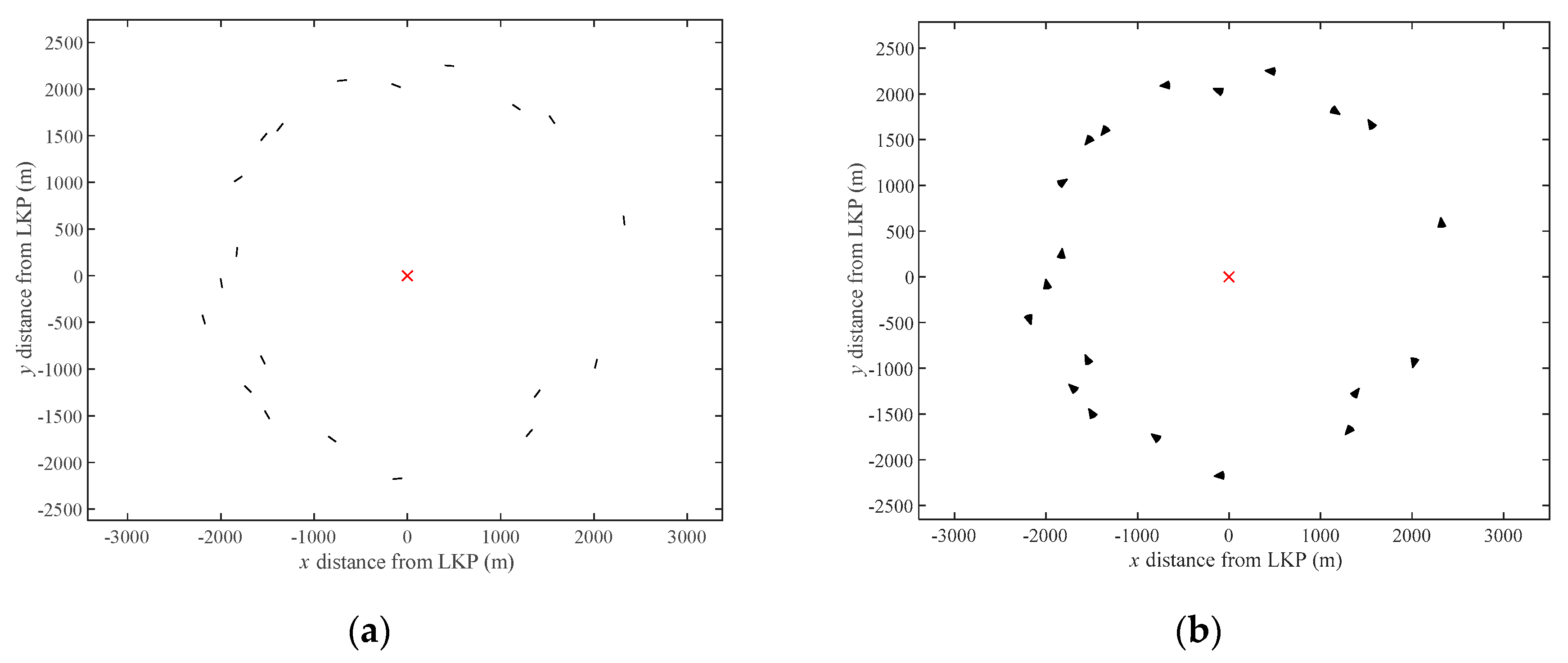
4.1.1. Phase 1: Off-Line Network Planning

The off-line network is planned using n = 50 sensors, each with a sensing range of R_s = 30 m. The search resources are available to deploy at t_start = 1800 s and the search commander has determined an end of search time of t_end = 7200 s.

The network-deployment planning begins with the simulation of 10,000 target motion trajectories, in Step 1.1, using the parameters of the demographic group to which the lost person belongs. For our example, the target walking speeds along the potential paths were sampled from a normal distribution with a mean of 0.5 m/s and a standard deviation of 0.167 m/s. The segments, of the target motions, were created using σ_θ = π/3 and d_m = 100 m. These parameters are the same as that of our target to ensure the simulated trajectories reflect the characteristics of their demographic.

Sensor poses were planned sequentially by first determining an optimal sub-region and corresponding deployment time, in Step 1.2, and, then, determining an optimal pose within this sub-region in Step 1.3 and, finally, constructing the linear-directional sensor from the linear one planned in the previous step. This yielded the positions {(x₁, y₁), …, (x₅₀, y₅₀)}, orientations, {θ₁, …, θ₅₀} and corresponding placement times, {t₁, …, t₅₀} for all n sensors in sorted order with t₁ being the earliest deployment and t₅₀ being the latest. The original deployment plan is shown in Figure 11.

4.1.2. Phase 2: Network Deployment Execution

The deployment plan is, then, executed. However, a clue is found at t = 2355 s at (−1330, −795). At this time, 25 of the original 50 sensors have been deployed. As a result of the clue find, the third phase of the deployment is invoked where the network is re-planned for the remaining sensors according to the updated LKP.

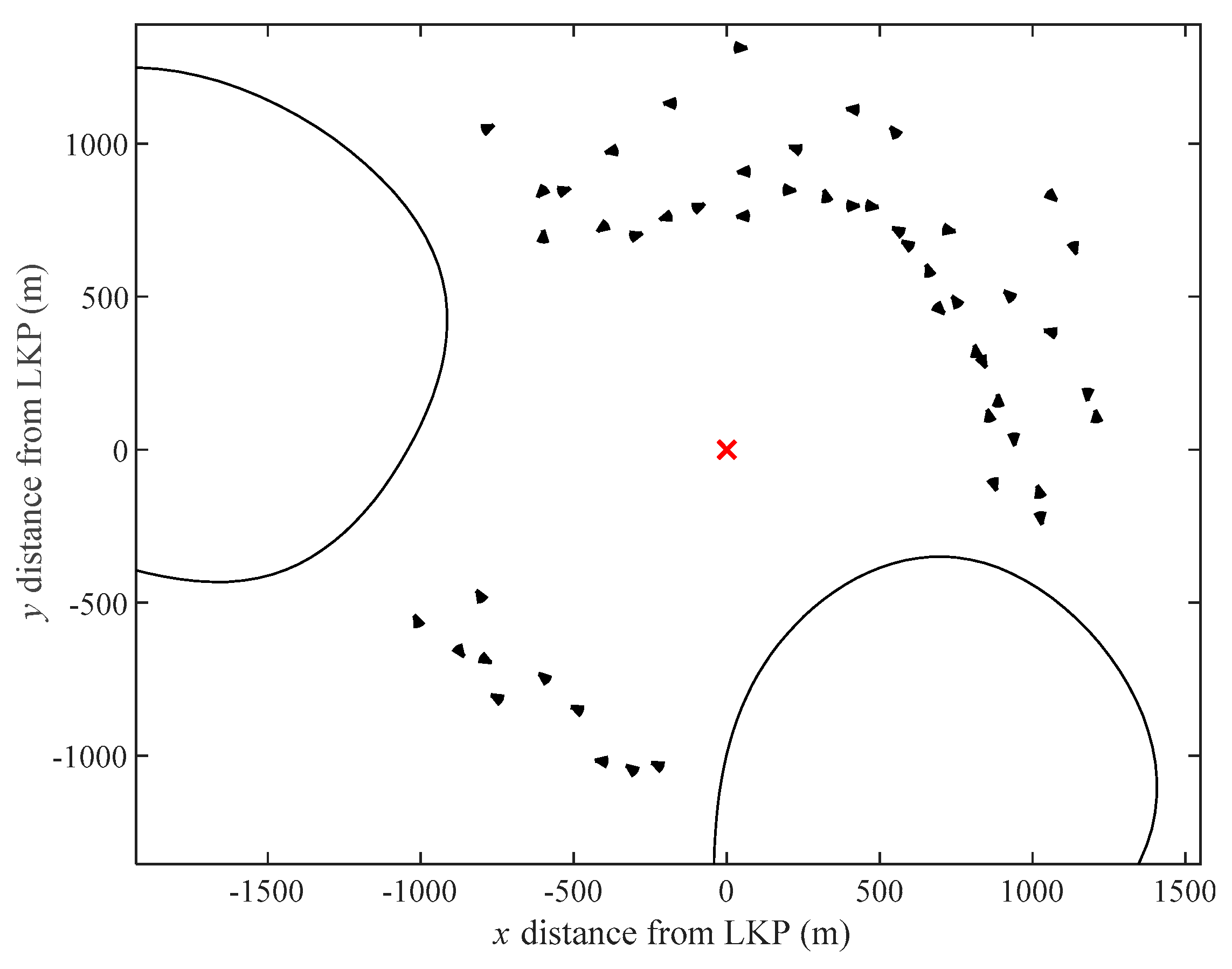
4.1.3. Phase 3: Network Re-Planning

A conservative estimate of the expected time of arrival, using the maximum target speed and the straight-line distance to the clue position, of the target is 1550 s. A deployment plan, centered at this new LKP, is simulated to determine the poses for the remaining 25 sensors. Figure 12 shows the full deployment plan including the original and re-planned poses of the sensors.

The deployment plan is restarted at t₂₆ = 2450 s. The search continued until the target was eventually detected by a re-planned sensor at t = 4850 s, at the position (−1895, −1260). Figure 13 shows a four-frame movie strip from t = 2450 s until the time of interception t = 4850 s.

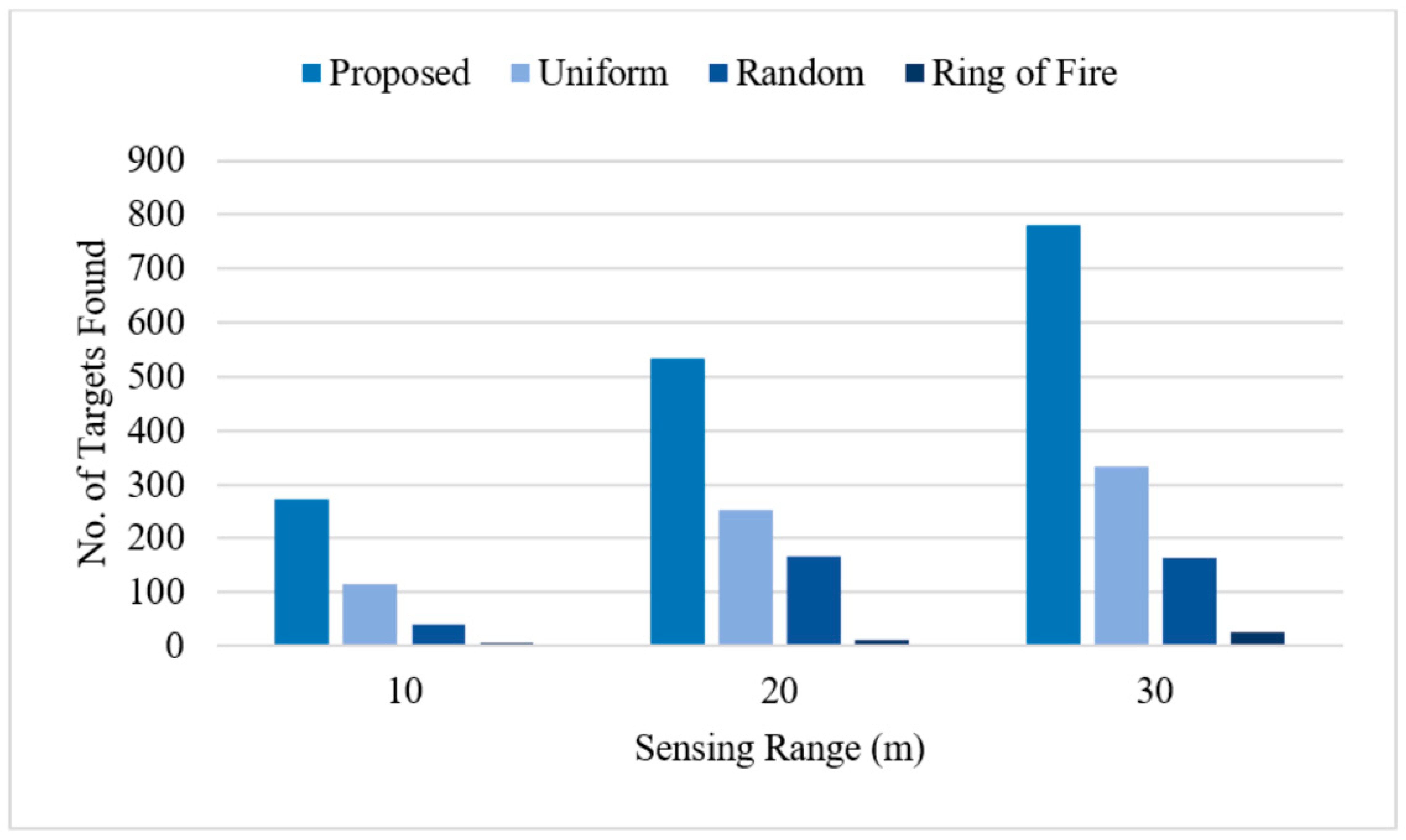
4.2. Comparative Study against Standard Topologies

In order to demonstrate its effectiveness, the proposed deployment methodology was evaluated against several existing deployment strategies. However, no static directional sensor deployment methodologies for mobile target detection exist in the present literature. Furthermore, existing DSN literature does not consider sparse coverage with temporal constraints and as a result a direct competitor cannot be established.

Thus, as a benchmark, herein, our proposed strategy was compared against three common deployment methods: (a) uniform [82], (b) random [83,84], and (c) a ‘ring of fire’ type deployment, which is inspired by the expected topology in a border surveillance application, where search resources are arranged to form a single, air-tight, barrier around a point of interest (i.e., the LKP) [53,54,55,56].

Uniform sensor networks are, typically, deployed by dividing the RoI into either square, triangular or hexagonal grid-based patterns and deploying along the grid vertices [82]. In contrast, our approach utilizes a gradient-based optimization [85]. The optimization evenly spaces out randomly generated deployment positions within a bounded region until a convergence criterion is met. This was practically implemented using the fmincon function in MATLAB’s optimization toolbox. The size of the bounded region is found by determining the furthest distance a target, with the specified demographics, could have travelled by the end of search time, t_end. Directional sensors are, then, deployed at these positions and oriented perpendicular to the LKP as this is the orientation expected to maximize trajectory intersections; this approach is also taken in the random and ring of fire deployments.

For the randomly deployed network, sensor positions are found using random distributions. The random distribution for positions has limits to ensure that each sensor is within the specified region; same as that of the uniform deployment. This type of topology is often used within mobile sensor networks as an initial configuration from which adjustments are made to reach an optimal configuration, based on a target metric such as coverage or connectivity [86]. However, as we are only considering static sensors, the random poses of the sensors represent their final configuration.

The ring of fire network is determined by arranging the available sensors into the largest possible, air-tight, circular boundary around the LKP.

Figure 14 below shows example topologies of the four deployment methods found using 50 sensors with 100 m sensing ranges for a t_start = 3600 s and a t_end = 7200 s.

The sensor network plans of our proposed methodology and the comparative models were tested with the same set of 10,000 trajectories. These represent the test trajectories, n_t, from our estimator of success, which was introduced in Equation (2). The performance of each model was evaluated by determining how many trajectories their respective plans were able to intersect, n_td. This was repeated a number of times and averaged to remove performance bias on any particular set of 10,000 trajectories. The test trajectories were simulated with a mean target walking speed of 0.7 m/s and a standard deviation of 0.23 m/s. The segments, of the target motions, were created using σ_θ = π/3 and d_m = 100 m. For our proposed methodology, the sensors were delivered by 3 delivery robots that travel at a constant speed of 10 m/s. It is assumed that the sensors are deployed all at once for the three benchmark methods (i.e., the deployment time for all of the sensors is the same as the deployment start time t_start = 3600 s).

The results for the comparative study (i.e., the values of n_td achieved by each sensor network plan) are shown for a deployment start time of 1800 s in Figure 15 and Figure 16 and for a start time of 3600 s in Figure 17 and Figure 18, respectively. The end of search time was 5400 s and 7200 s, respectively.

From the results, it is clear that the proposed methodology outperforms all three of the benchmark methods. As expected, a larger sensing range or number of sensors increases the number of targets found. Furthermore, it can be seen that the earlier the deployment starts, a higher total number of targets can be intercepted. This is expected as deploying earlier in the targets’ trajectories means that they will be closer together and a single deployment will be able to intersect a higher number of trajectories.

In the best case, with a deployment start time of 1800 s and 100 sensors with a 20 m sensing range, the proposed methodology outperforms the next best method, the uniform deployment, by 48% (i.e., it intercepts almost twice as many targets). In the worst case, with a start time of 3600 s and 20 sensors with a 20 m sensing range, the proposed strategy is still able to intercept 3.2 times as many targets as the next best model, the uniform deployment.

It should be noted that the ring of fire method will outperform the other methods if a large enough number of resources is available to form an air-tight barrier around all the simulated trajectories. However, the performance of this method diminishes with an increasing deployment start time as the targets have more time to move beyond the barrier. Furthermore, if the target is slower than anticipated, it may be a long time until they reach the ring of fire barrier which is not ideal in a time-critical application such as WiSAR.

In addition to having a higher performance, in terms of target detection probability, the proposed methodology also benefits from being adaptable to new target information. This improves upon traditional static-sensor strategies that deploy at a single optimal deployment time. By being adaptable, the cost of opportunities lost is avoided.

5. Conclusions

In this paper, we present a novel directional static-sensor deployment strategy for mobile-target detection. Optimal deployment poses planned, utilizing the concept of linear sensing models, are determined by positioning sensors in areas of high target densities, in orientations that maximize the number of trajectory intersections. The feasibility of sensor delivery is considered by ensuring that a sensor can be delivered, at the optimal sub-region, by one of the available delivery robots. The proposed time-phased strategy is adaptive, in that the deployment plan can be altered if new information becomes available during the network-deployment execution.

The proposed solution methodology is also applicable to problems beyond WiSAR. For example, the solution to the novel mathematical problem could be used for urban planning where a highway needs to intersect several roads or for planning additional connections to a complex network of pipelines. The density estimation approach, used to determine an optimal sub-region, could be used for applications that require determining priority areas, within a bounded region, to optimize for a specified metric. Conversely, the approach could be used to determine areas to avoid by locating regions with high densities of a specified metric.

References

1. Akyildiz, I.F.; Su, W.; Sankarasubramaniam, Y.; Cayirci, E. Wireless Sensor Networks: A Survey. Comput. Netw. 2002, 38, 30. [Google Scholar] [CrossRef] [Green Version]
2. Serna, M.A.; Casado, R.; Bermúdez, A.; Pereira, N.; Tennina, S. Distributed Forest Fire Monitoring Using Wireless Sensor Networks. Int. J. Distrib. Sens. Networks 2015, 2015, 1–18. [Google Scholar] [CrossRef]
3. Xu, Y.-H.; Sun, Q.-Y.; Xiao, Y.-T. An Environmentally Aware Scheme of Wireless Sensor Networks for Forest Fire Monitoring and Detection. Future Internet 2018, 10, 102. [Google Scholar] [CrossRef] [Green Version]
4. Kadri, B.; Bouyeddou, B.; Moussaoui, D. Early Fire Detection System Using Wireless Sensor Networks. In Proceedings of the 2018 International Conference on Applied Smart Systems (ICASS), Medea, Algeria, 24–25 November 2018; pp. 1–4. [Google Scholar]
5. Ramesh, M.V. Design, development, and deployment of a wireless sensor network for detection of landslides. Ad Hoc Netw. 2014, 13, 2–18. [Google Scholar] [CrossRef]
6. Li, X.; Zhang, X.; Guo, B. Application of Collocated GPS and Seismic Sensors to Earthquake Monitoring and Early Warning. Sensors 2013, 13, 14261–14276. [Google Scholar] [CrossRef] [PubMed] [Green Version]
7. Sun, Z.; Wang, P.; Vuran, M.C.; Al-Rodhaan, M.A.; Al-Dhelaan, A.M.; Akyildiz, I.F. BorderSense: Border patrol through advanced wireless sensor networks. Ad Hoc Netw. 2011, 9, 468–477. [Google Scholar] [CrossRef] [Green Version]
8. Cashbaugh, J.; Kitts, C. Optimizing Sensor Locations in a Multisensor Single-Object Tracking System. Int. J. Distrib. Sens. Netw. 2015, 11, 741491. [Google Scholar] [CrossRef]
9. Akter, M.; Rahman, O.; Islam, N.; Hassan, M.M.; AlSanad, A.; Sangaiah, A.K. Energy-Efficient Tracking and Localization of Objects in Wireless Sensor Networks. IEEE Access 2018, 6, 17165–17177. [Google Scholar] [CrossRef]
10. Wen, Y.; Gao, R.; Zhao, H. Energy Efficient Moving Target Tracking in Wireless Sensor Networks. Sensors 2016, 16, 29. [Google Scholar] [CrossRef]
11. Ochoa, S.F.; Santos, R.M. Human-centric wireless sensor networks to improve information availability during urban search and rescue activities. Inf. Fusion 2015, 22, 71–84. [Google Scholar] [CrossRef]
12. Erdelj, M.; Król, M.; Natalizio, E. Wireless Sensor Networks and Multi-UAV systems for natural disaster management. Comput. Netw. 2017, 124, 72–86. [Google Scholar] [CrossRef]
13. Francisco, J.; Fernando, G.-H.; Carlos, L.-A. A Coordinated Wilderness Search and Rescue Technique Inspired by Bacterial Foraging Behavior. In Proceedings of the 2018 IEEE International Conference on Robotics and Biomimetics (ROBIO), Kuala Lumpur, Malaysia, 12–15 December 2018; pp. 318–324. [Google Scholar]
14. Shin, J.C.L.; Kashino, Z.; Nejat, G.; Benhabib, B. A Sensor-Network-Supported Mobile-Agent-Search Strategy for Wilderness Rescue. Robotics 2019, 8, 61. [Google Scholar] [CrossRef] [Green Version]
15. Guvensan, M.A.; Yavuz, A.G. On coverage issues in directional sensor networks: A survey. Ad Hoc Netw. 2011, 9, 1238–1255. [Google Scholar] [CrossRef]
16. Plarre, K.; Kumar, P.R. Tracking Objects with Networked Scattered Directional Sensors. EURASIP J. Adv. Signal Process. 2007, 2008, 360912. [Google Scholar] [CrossRef] [Green Version]
17. Guvensan, M.A.; Yavuz, A.G. A New Coverage Improvement Algorithm Based on Motility Capability of Directional Sensor Nodes. In Ad-hoc, Mobile, and Wireless Networks; Springer: Berlin/Heidelberg, Germany, 2011; Volume 6811, pp. 206–219. [Google Scholar]
18. Wu, C.-H.; Chung, Y.-C. A tiling-based approach for directional sensor network deployment. 2010 IEEE Sens. 2010, 1358–1363. [Google Scholar] [CrossRef]
19. Liang, C.-K.; Tsai, C.-H.; He, M.-C. On area coverage problems in directional sensor networks. In Proceedings of the The International Conference on Information Networking 2011 (ICOIN2011), Barcelona, Spain, 26–28 January 2011; pp. 182–187. [Google Scholar]
20. Sung, T.-W.; Lu, Y.-T.; Lin, F.-T.; Yang, C.-S. Direction Control Using Delaunay Triangulation for Coverage Improvement in Directional Sensor Networks. In Proceedings of the 2015 Third International Conference on Robot, Vision and Signal Processing (RVSP), Kaohsiung, Taiwan, 18–20 November 2015; pp. 290–293. [Google Scholar]
21. Sung, T.-W.; Yang, C.-S. Distributed Voronoi-Based Self-Redeployment for Coverage Enhancement in a Mobile Directional Sensor Network. Int. J. Distrib. Sens. Netw. 2013, 9, 165498. [Google Scholar] [CrossRef]
22. Han, X.; Cao, X.; Lloyd, E.L.; Shen, C.-C. Deploying Directional Sensor Networks with Guaranteed Connectivity and Coverage. In Proceedings of the 2008 5th Annual IEEE Communications Society Conference on Sensor, Mesh and Ad Hoc Communications and Networks, San Francisco, CA, USA, 16–20 June 2008; pp. 153–160. [Google Scholar]
23. Chen, U.-R.; Chiou, B.-S.; Chen, J.-M.; Lin, W. An Adjustable Target Coverage Method in Directional Sensor Networks. In Proceedings of the 2008 IEEE Asia-Pacific Services Computing Conference, Yilan, Taiwan, 9–12 December 2008; pp. 174–180. [Google Scholar]
24. Akbarzadeh, V.; Gagné, C.; Parizeau, M.; Argany, M.; Mostafavi, M.A. Probabilistic Sensing Model for Sensor Placement Optimization Based on Line-of-Sight Coverage. IEEE Trans. Instrum. Meas. 2012, 62, 293–303. [Google Scholar] [CrossRef]
25. Wang, J.; Niu, C.; Shen, R. Priority-based target coverage in directional sensor networks using a genetic algorithm. Comput. Math. Appl. 2009, 57, 1915–1922. [Google Scholar] [CrossRef] [Green Version]
26. Singh, P.; Mini, S. A Heuristic to Deploy Directional Sensor Nodes in Wireless Sensor Networks. In Proceedings of the 2016 8th International Conference on Computational Intelligence and Communication Networks (CICN), Tehri, India, 23–25 December 2016; pp. 11–15. [Google Scholar]
27. Osais, Y.E.; St-Hilaire, M.; Yu, F.R. Directional Sensor Placement with Optimal Sensing Range, Field of View and Orientation. Mob. Netw. Appl. 2009, 15, 216–225. [Google Scholar] [CrossRef]
28. Varposhti, M.; Saleh, P.; Afzal, S.; Dehghan, M. Distributed area coverage in mobile directional sensor networks. In Proceedings of the 2016 8th International Symposium on Telecommunications (IST), Tehran, Iran, 26–27 September 2016; pp. 18–23. [Google Scholar] [CrossRef]
29. Ma, H.; Liu, Y. On Coverage Problems of Directional Sensor Networks. In Lecture Notes in Computer Science; Springer: Berlin/Heidelberg, Germany, 2005; pp. 721–731. [Google Scholar]
30. Cortes, J.; Martinez, S.; Karatas, T.; Bullo, F. Coverage Control for Mobile Sensing Networks. IEEE Trans. Robot. Autom. 2004, 20, 243–255. [Google Scholar] [CrossRef]
31. Ganguli, A.; Cortés, J.; Bullo, F. Distributed Coverage of Nonconvex Environments. In Networked Sensing Information and Control; Saligrama, V., Ed.; Springer: Boston, MA, USA, 2008; pp. 289–305. [Google Scholar]
32. Kantaros, Y.; Zavlanos, M.M. Distributed communication-aware coverage control by mobile sensor networks. Automatica 2016, 63, 209–220. [Google Scholar] [CrossRef]
33. Gusrialdi, A.; Hatanaka, T.; Fujita, M. Coverage control for mobile networks with limited-range anisotropic sensors. In Proceedings of the 2008 47th IEEE Conference on Decision and Control, Cancun, Mexico, 9–11 December 2008; pp. 4263–4268. [Google Scholar]
34. Stergiopoulos, Y.; Tzes, A. Cooperative positioning/orientation control of mobile heterogeneous anisotropic sensor networks for area coverage. In Proceedings of the 2014 IEEE International Conference on Robotics and Automation (ICRA), Hong Kong, China, 31 May–7 June 2014; pp. 1106–1111. [Google Scholar] [CrossRef]
35. Lee, S.G.; Diaz-Mercado, Y.; Egerstedt, M. Multirobot Control Using Time-Varying Density Functions. IEEE Trans. Robot. 2015, 31, 489–493. [Google Scholar] [CrossRef]
36. Miah, S.; Panah, A.Y.; Fallah, M.M.H.; Spinello, D. Generalized non-autonomous metric optimization for area coverage problems with mobile autonomous agents. Automatica 2017, 80, 295–299. [Google Scholar] [CrossRef]
37. Kennedy, J.; Chapman, A.; Dower, P.M. Generalized Coverage Control for Time-Varying Density Functions. In Proceedings of the 2019 18th European Control Conference (ECC), Naples, Italy, 25–28 June 2019; pp. 71–76. [Google Scholar]
38. Lekien, F.; Leonard, N.E. Nonuniform coverage and cartograms. In Proceedings of the 49th IEEE Conference on Decision and Control (CDC), Atlanta, GA, USA, 15–17 December 2010; pp. 5518–5523. [Google Scholar]
39. Amaldi, E.; Capone, A.; Cesana, M.; Filippini, I. Design of Wireless Sensor Networks for Mobile Target Detection. IEEE/ACM Trans. Netw. 2011, 20, 784–797. [Google Scholar] [CrossRef]
40. Clouqueur, T.; Phipatanasuphorn, V.; Ramanathan, P.; Saluja, K.K. Sensor Deployment Strategy for Detection of Targets Traversing a Region. Mob. Netw. Appl. 2003, 8, 453–461. [Google Scholar] [CrossRef]
41. Kashino, Z.; Vilela, J.; Kim, J.Y.; Nejat, G.; Benhabib, B. An adaptive static-sensor network deployment strategy for detecting mobile targets. In Proceedings of the 2016 IEEE International Symposium on Safety, Security, and Rescue Robotics (SSRR), Lausanne, Switzerland, 23–27 October 2016; pp. 1–8. [Google Scholar] [CrossRef]
42. Rogge, J.A.; Aeyels, D. Multi-robot coverage to locate fixed and moving targets. In Proceedings of the 2009 IEEE International Conference on Control Applications, St. Petersburg, Russia, 8–10 July 2009; pp. 902–907. [Google Scholar]
43. Grundel, D.A. Searching for a moving target: Optimal path planning. In Proceedings of the 2005 IEEE Networking, Sensing and Control, Tucson, AZ, USA, 19–22 March 2005; pp. 867–872. [Google Scholar]
44. Macwan, A.; Vilela, J.; Nejat, G.; Benhabib, B. A Multirobot Path-Planning Strategy for Autonomous Wilderness Search and Rescue. IEEE Trans. Cybern. 2014, 45, 1784–1797. [Google Scholar] [CrossRef]
45. Kashino, Z.; Nejat, G.; Benhabib, B. A Hybrid Strategy for Target Search Using Static and Mobile Sensors. IEEE Trans. Cybern. 2020, 50, 856–868. [Google Scholar] [CrossRef]
46. Li, X.; Fletcher, G.; Nayak, A.; Stojmenovic, I. Randomized carrier-based sensor relocation in wireless sensor and robot networks. Ad Hoc Netw. 2013, 11, 1951–1962. [Google Scholar] [CrossRef]
47. Kantaros, Y.; Schlotfeldt, B.; Atanasov, N.; Pappas, G.J. Asymptotically Optimal Planning for Non-Myopic Multi-Robot Information Gathering. In Proceedings of the Robotics: Science and Systems XV, Freiburg, Germany, 22–26 June 2019. [Google Scholar] [CrossRef]
48. Atanasov, N.; Le Ny, J.; Daniilidis, K.; Pappas, G.J. Decentralized active information acquisition: Theory and application to multi-robot SLAM. In Proceedings of the 2015 IEEE International Conference on Robotics and Automation (ICRA), Seattle, WA, USA, 26–30 May 2015; pp. 4775–4782. [Google Scholar]
49. Kumar, V.; Rus, D.; Singh, S. Robot and Sensor Networks for First Responders. IEEE Pervasive Comput. 2004, 3, 24–33. [Google Scholar] [CrossRef] [Green Version]
50. Kumar, A.A.; Sivalingam, K.M. Target tracking in a WSN with directional sensors using electronic beam steering. In Proceedings of the 2012 Fourth International Conference on Communication Systems and Networks (COMSNETS 2012), Bangalore, India, 3–7 January 2012; pp. 1–10. [Google Scholar]
51. Mohajerzadeh, A.H.; Jahedinia, H.; Izadi-Ghodousi, Z.; Abbasinezhad-Mood, D.; Salehi, M. Efficient target tracking in directional sensor networks with selective target area’s coverage. Telecommun. Syst. 2017, 68, 47–65. [Google Scholar] [CrossRef]
52. Tripathi, A.; Gupta, H.P.; Dutta, T.; Kumar, D.; Jit, S.; Shukla, K.K. A Target Tracking System Using Directional Nodes in Wireless Sensor Networks. IEEE Syst. J. 2019, 13, 1618–1627. [Google Scholar] [CrossRef]
53. Wang, Z.; Liao, J.; Cao, Q.; Qi, H.; Wang, Z. Barrier Coverage in Hybrid Directional Sensor Networks. In Proceedings of the 2013 IEEE 10th International Conference on Mobile Ad-Hoc and Sensor Systems, Hangzhou, China, 14–16 October 2013; pp. 222–230. [Google Scholar]
54. Zhao, L.; Bai, G.; Shen, H.; Tang, Z. Strong barrier coverage of directional sensor networks with mobile sensors. Int. J. Distrib. Sens. Netw. 2018, 14. [Google Scholar] [CrossRef] [Green Version]
55. Benahmed, T.; Benahmed, K. Optimal barrier coverage for critical area surveillance using wireless sensor networks. Int. J. Commun. Syst. 2019, 32, e3955. [Google Scholar] [CrossRef]
56. Liu, X.; Yang, B.; Chen, G. Full-view barrier coverage in mobile camera sensor networks. Wirel. Netw. 2018, 25, 4773–4784. [Google Scholar] [CrossRef]
57. Kashino, Z.; Nejat, G.; Benhabib, B. A multi-robot sensor-delivery planning strategy for static-sensor networks. In Proceedings of the 2017 IEEE/RSJ International Conference on Intelligent Robots and Systems (IROS), Vancouver, BC, Canada, 24–28 September 2017; pp. 6640–6647. [Google Scholar]
58. Wang, Y.; Wu, C.-H. Robot-Assisted Sensor Network Deployment and Data Collection. In Proceedings of the 2007 International Symposium on Computational Intelligence in Robotics and Automation, Jacksonville, FI, USA, 20–23 June 2007; pp. 467–472. [Google Scholar]
59. Shiu, L.C. The robot deployment scheme for wireless sensor networks in the concave region. In Proceedings of the 2009 International Conference on Networking, Sensing and Control, Okayama, Japan, 26–29 March 2009; pp. 581–586. [Google Scholar]
60. Fletcher, G.; Li, X.; Nayak, A.; Stojmenovic, I. Back-Tracking Based Sensor Deployment by a Robot Team. In Proceedings of the 2010 7th Annual IEEE Communications Society Conference on Sensor, Mesh and Ad Hoc Communications and Networks (SECON), Boston, MA, USA, 21–25 June 2010; pp. 1–9. [Google Scholar]
61. Wang, Y.-H.; Tsai, J.J.P.; Wu, Y.-H. Robot-based deployment mechanism for wireless sensor networks in unknown region. In Proceedings of the 2013 International Joint Conference on Awareness Science and Technology & Ubi-Media Computing (iCAST 2013 & UMEDIA 2013), Aizu-Wakamatsu, Japan, 2–4 November 2013; pp. 143–149. [Google Scholar]
62. Mesa-Barrameda, E.; Santoro, N.; Shi, W.; Taleb, N. Sensor deployment by a robot in an unknown orthogonal region: Achieving full coverage. In Proceedings of the 2014 20th IEEE International Conference on Parallel and Distributed Systems (ICPADS), Hsinchu, Taiwan, 16–19 December 2014; pp. 951–960. [Google Scholar]
63. Rajesh, M.; George, A.; Sudarshan, T.S.B. Energy efficient deployment of Wireless Sensor Network by multiple mobile robots. In Proceedings of the 2015 International Conference on Computing and Network Communications (CoCoNet), Trivandrum, India, 16–19 December 2015; pp. 72–78. [Google Scholar]
64. Batalin, M.A.; Sukhatme, G.S. Coverage, Exploration and Deployment by a Mobile Robot and Communication Network. Telecommun. Syst. 2004, 26, 181–196. [Google Scholar] [CrossRef]
65. Tuna, G.; Gungor, V.C.; Gulez, K. An autonomous wireless sensor network deployment system using mobile robots for human existence detection in case of disasters. Ad Hoc Netw. 2014, 13, 54–68. [Google Scholar] [CrossRef]
66. Woiceshyn, K.; Kashino, Z.; Nejat, G.; Benhabib, B. Vehicle Routing for Resource Management in Time-Phased Deployment of Sensor Networks. IEEE Trans. Autom. Sci. Eng. 2018, 16, 716–728. [Google Scholar] [CrossRef]
67. Wang, Z.; Zhao, X.; Qian, X. Carrier-based sensor deployment by a mobile robot for wireless sensor networks. In Proceedings of the 2012 12th International Conference on Control Automation Robotics & Vision (ICARCV), Guangzhou, China, 5–7 December 2012; pp. 1663–1668. [Google Scholar]
68. Kashino, Z.; Kim, J.Y.; Nejat, G.; Benhabib, B. Spatiotemporal Adaptive Optimization of a Static-Sensor Network via a Non-Parametric Estimation of Target Location Likelihood. IEEE Sens. J. 2017, 17, 1479–1492. [Google Scholar] [CrossRef]
69. Vilela, J.; Kashino, Z.; Ly, R.; Nejat, G.; Benhabib, B. A Dynamic Approach to Sensor Network Deployment for Mobile-Target Detection in Unstructured, Expanding Search Areas. IEEE Sens. J. 2016, 16, 4405–4417. [Google Scholar] [CrossRef]
70. Yanmaz, E.; Guclu, H. Stationary and Mobile Target Detection Using Mobile Wireless Sensor Networks. In Proceedings of the 2010 INFOCOM IEEE Conference on Computer Communications Workshops, San Diego, CA, USA, 15–19 March 2010; pp. 1–5. [Google Scholar] [CrossRef] [Green Version]
71. Zou, Y.; Chakrabarty, K. Sensor deployment and target localization in distributed sensor networks. ACM Trans. Embed. Comput. Syst. 2004, 3, 61–91. [Google Scholar] [CrossRef]
72. Koester, R.J. Lost Person Behavior: A Search and Rescue Guide on where to Look for Land, Air, and Water; dbS Productions: Charlottesville, VA, USA, 2008. [Google Scholar]
73. Lin, L.; Goodrich, M.A. A Bayesian approach to modeling lost person behaviors based on terrain features in Wilderness Search and Rescue. Comput. Math. Organ. Theory 2010, 16, 300–323. [Google Scholar] [CrossRef]
74. Hooke, R.; Jeeves, T.A. Direct Search Solution of Numerical and Statistical Problems. J. ACM 1961, 8, 212–229. [Google Scholar] [CrossRef]
75. Garai, G.; Chaudhuri, B. A distributed hierarchical genetic algorithm for efficient optimization and pattern matching. Pattern Recognit. 2007, 40, 212–228. [Google Scholar] [CrossRef]
76. Yun, Z.; Bai, X.; Xuan, D.; Lai, T.H.; Jia, W. Optimal Deployment Patterns for Full Coverage and k-Connectivity (k ≤ 6) Wireless Sensor Networks. IEEE/ACM Trans. Netw. 2010, 18, 934–947. [Google Scholar] [CrossRef]
77. Gupta, H.P.; Tyagi, P.K.; Singh, M.P. Regular Node Deployment for k-Coverage in mm-Connected Wireless Networks. IEEE Sens. J. 2015, 15, 7126–7134. [Google Scholar] [CrossRef]
78. Sakai, K.; Sun, M.-T.; Ku, W.-S.; Lai, T.-H.; Vasilakos, A.V. A Framework for the Optimal k-Coverage Deployment Patterns of Wireless Sensors. IEEE Sens. J. 2015, 15, 7273–7283. [Google Scholar] [CrossRef]
79. Lagarias, J.C.; Reeds, J.A.; Wright, M.H.; Wright, P.E. Convergence Properties of the Nelder--Mead Simplex Method in Low Dimensions. SIAM J. Optim. 1998, 9, 112–147. [Google Scholar] [CrossRef] [Green Version]
80. Jou, E.D. Determine Whether Two Line Segments Intersect. In Modeling in Computer Graphics, Proceedings of the IFIP WG 5.10 Working Conference Tokyo, Japan, 8–12 April 1991; Kunii, T.L., Ed.; Springer: Tokyo, Japan, 1991; pp. 265–274. [Google Scholar]
81. Künsch, H.R. Particle filters. Bernoulli 2013, 19, 1391–1403. [Google Scholar] [CrossRef] [Green Version]
82. Biagioni, E.; Sasaki, G. Wireless sensor placement for reliable and efficient data collection. In Proceedings of the 36th Annual Hawaii International Conference on System Sciences, Big Island, HI, USA, 6–9 January 2003; p. 10. [Google Scholar]
83. Zou, Y.; Chakrabarty, K. Sensor deployment and target localization based on virtual forces. In Proceedings of the IEEE INFOCOM Twenty-second Annual Joint Conference of the IEEE Computer and Communications Societies (IEEE Cat. No.03CH37428), San Francisco, CA, USA, 30 March–3 April 2003; Volume 2, pp. 1293–1303. [Google Scholar]
84. Rout, M.; Roy, R. Dynamic deployment of randomly deployed mobile sensor nodes in the presence of obstacles. Ad Hoc Netw. 2016, 46, 12–22. [Google Scholar] [CrossRef]
85. Han, S.P. A globally convergent method for nonlinear programming. J. Optim. Theory Appl. 1977, 22, 297–309. [Google Scholar] [CrossRef] [Green Version]
86. Tan, G.; Jarvis, S.A.; Kermarrec, A.-M. Connectivity-Guaranteed and Obstacle-Adaptive Deployment Schemes for Mobile Sensor Networks. Available online: https://hal.inria.fr/inria-00432129/document (accessed on 6 October 2020).
Figure 1. (a) A traditional directional sensing model; and, (b) the proposed linear sensing model (α = 0).
Robotics 09 00082 g001
Figure 2. Original network deployment procedure.
Robotics 09 00082 g002
Figure 3. A set of 100 target trajectories between (a) t = 0 and tend = 7200 s (b) tstart = 3600 s and tend = 7200 s.
Robotics 09 00082 g003
Figure 4. The hexagonal pattern used to determine the region with the maximum density of trajectories in its (a) initial, (b) a first intermediary, (c) a second intermediary, and (d) final configurations, respectively.
Robotics 09 00082 g004
Figure 5. Determining deployment time using the respective positions of three delivery robots from the center of a deployment sub-region.
Robotics 09 00082 g005
Figure 6. An example of orientation optimization within a sub-region.
Robotics 09 00082 g006
Figure 7. A single sensor network planned utilizing a (a) linear sensing model and converted to (b) a directional sensor network.
Robotics 09 00082 g007
Figure 8. The original DSN deployment topology noted in Table 1.
Robotics 09 00082 g008
Figure 9. DSN redeployment after a clue find.
Robotics 09 00082 g009
Figure 10. The target path if not intercepted by the search.
Robotics 09 00082 g010
Figure 11. The original deployment plan.
Robotics 09 00082 g011
Figure 12. The full deployment including the original and re-planned sensors.
Robotics 09 00082 g012
Figure 13. The search at various times after the clue find (a) 2448 s, (b) 2512 s, (c) 2686 s, and (d) 4850 s.
Robotics 09 00082 g013aRobotics 09 00082 g013b
Figure 14. The topologies of the (a) proposed deployment, (b) uniform deployment, (c) random deployment and, (d) ring of fire deployment.
Robotics 09 00082 g014
Figure 15. The number of targets found by a set of 50 sensors with varying sensing ranges and a deployment start time of 1800 s.
Robotics 09 00082 g015
Figure 16. The number of targets found by topologies of a varying number of sensors with a sensing range of 20 m and a deployment start time of 1800 s.
Robotics 09 00082 g016
Figure 17. The number of targets found by a set of 50 sensors with varying sensing ranges and a deployment start time of 3600 s.
Robotics 09 00082 g017
Figure 18. The number of targets found by topologies of a varying number of sensors with a sensing range of 20 m and a deployment start time of 3600 s.
Robotics 09 00082 g018