Abstract
This article presents the development of a fuzzy guidance system (FGS) for unmanned aerial vehicles capable of pursuing and performing rendezvous with static and mobile targets. The system is designed to allow the vehicle to approach a maneuvering target from a desired direction of arrival and to terminate the rendezvous at a constant distance from the target. In order to perform a rendezvous with a maneuvering target, the desired direction of arrival is adjusted over time to always approach the target from behind, so that the aircraft and target velocity vectors become aligned. The proposed guidance system assumes the presence of an autopilot and uses a set of Takagi–Sugeno fuzzy controllers to generate the orientation and speed references for the velocity and heading control loops, given the relative position and velocity between the aircraft and the target. The FGS treats the target as a mobile waypoint in a 4-D space (position in 2-dimensions, desired crossing heading and speed) and guides the aircraft on suitable trajectories towards the target. Only when the vehicle is close enough to the rendezvous point, the guidance law is complemented with an additional linear controller to manage the terminal formation keeping phase. The capabilities of the proposed rendezvous-FGS are verified in simulation on both maneuvering and non-maneuvering targets. Finally, experimental results using a multi-rotor aerial system are presented for both fixed and accelerating targets.
1. Introduction
The pursuit and rendezvous processes consist of a series of maneuvers that bring a chaser towards its target. Pursuit refers usually to the process of chasing a target and reaching it without specific requirements on the value of the relative velocity vector at the intercept point, such as, for instance, for missile guidance [1]. Rendezvous refers usually instead to the process of getting at a same place and at the same time with a target and with zero relative velocity, so that motion in formation, docking or other operations may follow [2]. Pursuit and rendezvous controllers are then fundamental for all those applications which require one to approach, follow and encounter a specific target that can be static or in motion, cooperative or not.
There are various applications that require a vehicle to approach another vehicle and span from the marine [3,4,5], ground [6] and space [2,7,8] fields, and, in general, are managed in very different ways depending on the range of admissible initial conditions, on the solution approach, but also depending on the dynamics that describe the relative motion between the two bodies.
In general, there are approaches that focus mainly on the final phase, where the relative distance is small, trajectory errors may lead to collisions, and relative dynamics can be linearized [9,10], while other approaches focus instead on defining the path that leads to the rendezvous rather than the final phase only. This latter problem can be faced in various ways like, for instance, using path planning techniques [11], closed loop optimal control techniques like model predictive control [12], or guidance techniques derived from missile intercept guidance laws [13,14].
An all-encompassing comparison with all approaches for pursuit and rendezvous with respect to some target is not possible here and it is outside the scope of this paper; thus, a brief review is proposed of existing approaches that face exactly our same guidance problem or one very similar to it, with a focus on state-of-the-art and most recent results.
This paper proposes a system capable of intercepting or performing rendezvous with an accelerating target with a time-varying desired angle of arrival, where the approach path characteristics and shape are defined during the system design. The proposed method generates the necessary vehicle velocity vector using a set of fuzzy systems and its output is supposed to be used as input into the vehicle’s autopilot. The basic idea behind the proposed approach has been developed and employed by several authors in the past. One of the first appearances of a Fuzzy Guidance System is [15] where the author proposes a fuzzy map for waypoint guidance for fized waypoints with desired angle of arrival capable of handling any possible initial condition. In [16] the authors propose a fuzzy guidance system (FGS) for underwater vehicles docking to a still submarine that is capable though of managing arrival from behind only. The authors of [3] and [17] propose a FGS for docking to a fixed underwater station also in the presence of underwater currents. This latter case is managed using a model-based current/disturbance estimator. Another work [18] presents a FGS designed for approach to and docking with a fixed target and they test it with a slowly moving target. It should be noted that none of the fuzzy guidance systems proposed so far can explicitly handle accelerating targets or a time-varying direction of arrival as instead is the FGS developed in this paper. The peculiarity that makes all the above methods similar is that they shape the approach trajectory to the target in closed loop as a function of relative kinematic variables (position, velocity etc.), so they are actually guidance systems where the desired approach path characteristics are embedded at design time in the system.
For the sake of clairity and completeness, many other approaches are proposed in the literature under the name fuzzy guidance, even if they have little in common with those presented above; a recent survey [19] contains several examples of so-called fuzzy guidance approaches that, nonetheless, should be more precisely considered “controllers” and not “guidance systems”, since the vehicle trajectory is not obtained from the guidance system, but is generated elsewhere and is rather an input to it. The methods analyzed in [19] have the goal to regulate and track trajectory-related variables with fuzzy techniques rather than actually generating the trajectory. We acknowledge that this is just a naming issue of little relevance, but, for the reason above, a direct comparison with this kind of fuzzy guidance systems is outside the scope of this paper.
It is therefore worth it to compare the proposed approach with similar approaches that do not use fuzzy logic but indeed share the same paradigm of guidance toward a target by shaping the approach trajectory in closed loop. Several approaches for guidance with a constraint on the angle of arrival exist [20,21,22] but these are designed specifically for missile application, and thus for intercept, they do not pose much attention to the shape of the obtained trajectory, but more on the feasibility of it withstanding the performance limit of the missile, and for all these reasons, modifications to achieve rendezvous may be very difficult. Modifications of missile guidances for rendezvous were proposed [13,14], but cannot handle a large set of possible initial conditions. Furthermore, as these are designed for missile application, the guidance output is an acceleration command, rather than a velocity vector command, that makes application to UAVs equipped with autopilots more complex and less natural. Other non-fuzzy guidance methods that do not regulate the state to predefined trajectories, but exploit similar velocity vector map paradigms fall under the name of vector fields (VFs) methods. This is a large family of methods that are often used also to avoid obstacles using so-called potential fields [23] or virtual force fields [24]. Within this large family, the methods that can be directly compared to the FGS proposed in this paper, because of their characteristics, are the Lyapunov VF (LVF) and the gradient VF (GVF) methods. These methods, from different perspectives though, produce guidance commands that let the pursuer converge to straight paths, circular paths, or a combination of these by means of “artificial” vector fields.
Gradient vector field methods, like, for instance, [25] or [24], exploit artificially created vector fields, often mimicking gradients of the electric field created by charged particles, to generate paths that the chaser must follow. To the authors’ knowledge no specific results exist with moving targets and desired direction of arrival. Originally proposed for stand-off tracking, that is circulating around a fixed or moving target [26,27], LVF methods have been recently proposed also for docking [28]; this latter work presented a LVF for an in-orbit approach and dock with a tumbling spacecraft. The two vehicles, pursuer and target, are on the same orbit, and this motivates the authors to design the guidance system on relative coordinates. Since the vehicles are moving in their orbit around the Earth, the target appears still, although tumbling to the chaser, and this simplifies the problem to docking to a stationary, non-accelerating target with time varying angle of arrival. In addition, as a correct assumption for a spacecraft, the chaser can follow arbitrary, although limited in norm, desired accelerations, but this makes application to an atmospheric flight vehicle more difficult. None of the above-referenced papers discussed the case of the accelerating target and only one [28] faced the problem of rotating direction of arrival.
This paper describes the development, implementation and experimental testing of a guidance scheme based on fuzzy systems that have been designed for pursuit and rendezvous with a mobile accelerating target. The desired angle of arrival may be changing in time, and, in particular, may be kept aligned with the target velocity vector to allow rendezvous and docking. The feasible approach path is generated by the guidance system in closed loop without any preliminary path planning. The proposed approach considers the kinematic constraint in the design phase, so that the problem of achieving a feasible path is solved in the system design phase. The FGS is designed to produce continuous and smooth trajectories, assuming that the vehicle knows its current position, target’s current position, as well as their velocity vectors. The target is described as a waypoint in a 4-dimensional space, position in two dimensions, desired crossing heading angle and desired crossing speed that is the speed the pursuer uses to approach the rendezvous point. This work extends the results of [29] where an FGS was proposed for static waypoints, targets in rectilinear motion and constant desired crossing direction, by explicitly considering maneuvering targets, time varying desired crossing direction and introducing the possibility to perform rendezvous with the target. The paper is organized as follows: Section 2 describes the general 4-dimensional FGS for waypoint/target interception; Section 3 describes the modifications needed to intercept accelerating targets, to manage time varying desired waypoint crossing direction and introduces the novel rendezvous-FGS with the support of simulation results. Finally, Section 4 presents some experimental results of the proposed rendezvous-FGS.
2. The Fuzzy Guidance System
2.1. General Definitions
The proposed guidance system is designed to generate a planar reference trajectory in terms of desired velocity vector , and the existence of an autopilot system that can track the desired commands on the plane and maintain constant the altitude of the vehicle is assumed; thus, vehicle speed and heading are regulated to the desired values by means of the internal control loops. The fuzzy guidance system (FGS) provides the external control loop and produces desired speed and heading for the autopilot. The position of the target is defined as a 2D waypoint in Cartesian coordinates expressed in an Earth-fixed reference system, with associated desired speed and heading angle that are used to define the approach path to the waypoint. The target waypoint defines a mobile coordinate frame centered in the waypoint position and rotated by the angle around the Z-axis with respect to the earth-fixed frame.
The waypoint-fixed coordinate system for convenience has the Y axis that points backwards from the prescribed crossing direction, as can be seen in Figure 1. The desired approach trajectory to the waypoint is achieved via the heading fuzzy controller , which generates the desired heading angle using the position errors along the X and Y axes of the current waypoint reference frame and using the heading error .
where is the rotation matrix between earth-fixed reference frame and waypoint fixed frame. Please note that, in order to reduce clutter in the equations, the explicit dependence on the time of most of the variables used throughout the paper will be omitted. Sporadically, the dependence on time will be indicated, where it is instrumental in highlighting time-varying quantities.
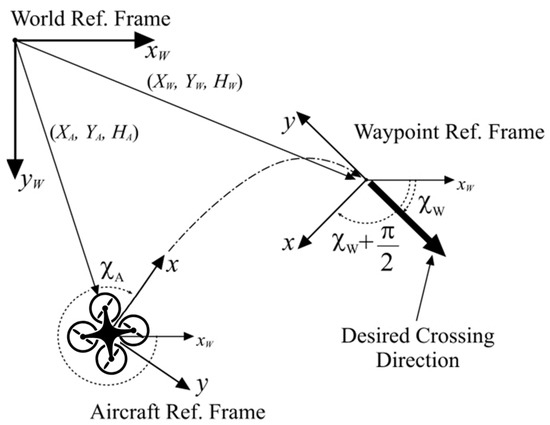
Figure 1.
Geometry of the guidance problem.
The fuzzy logic controller is designed to guide the vehicle towards the waypoint with a smooth trajectory and a desired crossing velocity. The desired heading angle produced by the heading controller in its general form is:
whereas the desired speed is function of the desired crossing speed , of vehicle velocity and target velocity vectors
The heading controllers are obtained using Takagi–Sugeno (TS) fuzzy systems [30] of the form:
where is the input vector and, is the i-th membership function that merges a set of fuzzy rules and is the output in the case of perfect rule matching. One important feature of the TS fuzzy systems described by Equation (5) is that their output realizes a static mapping of the input vector; furthermore, the mapping is a one-valued function of the input vector. Thus, a TS fuzzy system, once the design is finished, can be approximated with arbitrary accuracy with a look-up table for real-time implementation, and closed loop stability analysis of a linear system within a closed loop with a T-S FS can be performed using standard techniques [30,31]. The following section briefly describes the heading controller of the fuzzy guidance system, as was first presented in [29].
2.2. The Heading Controller
The heading controller is composed of two fuzzy systems: the fuzzy system generates the desired heading given the position in waypoint reference frame of the aircraft; working in the waypoint reference frame allows one to define desired trajectories around the waypoint (or target), regardless of the actual waypoint desired crossing direction. The output of the fuzzy system is summed with desired crossing heading of current waypoint to obtain the desired aircraft heading . The second fuzzy system is designed to improve the transient performance of the system, to manage the case of large heading errors, and to adapt the feedback gain depending on aircraft speed.
Figure 2 shows the resulting heading controller, where the trajectory heading error defines the error between current aircraft heading and the desired approach heading at the current aircraft position .
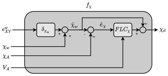
Figure 2.
Heading Controller composed by the two Fuzzy stages.
2.2.1. First Stage: Desired Route
The first fuzzy system generates the desired route expressed as the angle the aircraft velocity vector should have, with respect to the negative Y axis, in a specific point of the horizontal plane around the waypoint or target. Using a fuzzy system allows one to easily define a small set of plane areas and corresponding approach directions, that, merged with the fuzzy system, become a directions map that covers the entire plane. Thus, the membership functions and the fuzzy rules must be designed keeping into account maximum aircraft performance (e.g., minimum turn radius) and to obtain smooth maneuvers with limited control signals. In order to avoid undesirable steep variations of the desired route when passing from areas behind the waypoint to areas in front of it, the design was divided into two parts: guidance in the upper half plane and in the lower half plane () yielding two fuzzy systems: and .
For the purposes of this paper, the fuzzy guidance system described in [29] and originally conceived for airplanes has been redesigned for slower vehicles with much smaller turn radius.
The complete map of desired routes is obtained by smoothly joining the trajectories in the upper and lower planes along the X axis ( = 0) using the weighting function :
with
where = 0.5 [m].
The reference generated by the first stage becomes then:
The two fuzzy systems and both have 2 inputs: the position error and 1 output: the desired aircraft route. As the previous version of this FGS [29], the fuzzy system , is defined entirely by the 8 rules described in Table 1 (output values are in degrees) and by the membership functions shown in Figure 3a,b; the resulting nonlinear output characteristic is drawn in Figure 4.

Table 1.
Fuzzy Rules.
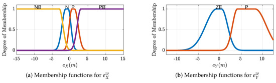
Figure 3.
Membership Functions for the fuzzy system .
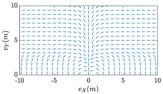
Figure 4.
Desired Routes in the Upper Plane generated by the fuzzy system .
The fuzzy system is defined entirely by the 7 rules which are described in Table 2 (output values are in degrees) and by the membership functions in Figure 5a,b. The resulting nonlinear output characteristic is drawn in Figure 6. For the sake of clarity, Table 1 and Table 2 contain the fuzzy output values of Equation (5) and each table cell should be interpret as follows, as an example consider upper left cell in Table 1:
Table 2.
Fuzzy Rules for .
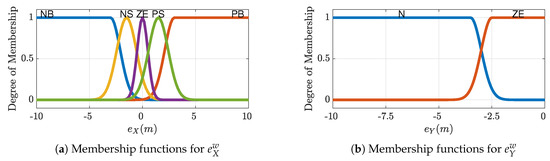
Figure 5.
Membership Functions for the fuzzy system .
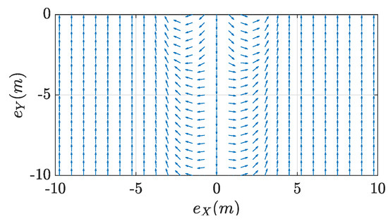
Figure 6.
Desired Routes in the Lower Plane generated by the fuzzy system .
- If is NB ∧ is ZE then is 90.
An asterisk instead indicates that the corresponding input condition has no associated output rule and that the result is obtained by interpolation of the results of the neighboring rules.
Note that the fuzzy maps were designed, for convenience, to have a symmetric output with respect to the Y axis of the waypoint frame, and that the output of the fuzzy system represents the desired heading correction with respect to the desired crossing direction that is set aligned with the negative Y axis (see Figure 1). As a matter of fact, when the aircraft is positioned behind the waypoint along the positive Y axis of the waypoint frame (that is is in the middle of the membership functions P and N), the output of the fuzzy system is 0 degrees, and since the desired direction produced by the fuzzy system is relative to the angle, then the desired aircraft heading angle is exactly . As a consequence of fuzzy system design then, the output of the fuzzy system is offset by the rotation of the negative Y axis with respect to the X waypoint axis, that is by , and this offset cancels with the term in Equation (1); this justifies why the latter does not appear in Equation (8) summed to .
2.2.2. Second Stage: Heading Error
Although the aircraft has a heading autopilot and thus the output of the first stage could be fed directly to it, the waypoint approach trajectory may not be correctly followed by the aircraft due to the transient response of the autopilot itself that is not taken into consideration in the first stage design; actually, the first stage fuzzy system is a static map between position and desired trajectory direction and, locally, is similar to a very simple proportional controller.
During an approach maneuver, the output of the first stage varies continuously; since, in general, an autopilot is not designed to track rapidly varying tracking references, the second stage of the heading controller was designed with the aim of improving the transient response and to limit the amount of heading error actually perceived by the autopilot. The second stage modifies the desired heading angle for the aircraft autopilot according to the aircraft heading error , and the current aircraft speed so that: the heading error never exceeds 90 degrees, small heading errors appear a little larger to speed up “slow” autopilots convergence to 0 heading error, and, at higher speeds, heading error appears larger than it actually is.
According to this idea, the fuzzy system was designed very similarly to the one described in [29] with a speed range between 1 and 5 m/s. The second stage output, that is the actual heading reference for the autopilot , is given by:
Figure 7 shows the input-output map of the fuzzy system that is clearly an odd function. Figure 7a shows a discretized 3D view of the fuzzy map, where it is evident that the contribution of the second stage becomes null when the heading error becomes null (i.e., ) and that the slope around zero heading error increases at higher velocity (the error perceived by the vehicle increases if it is advancing at higher speeds). Figure 7b shows a sample section of the fuzzy map obtained by setting the velocity to = 3 m/s. Reformulating Equation (9) as follows:
makes evident that the second stage helps keeping the heading error perceived by the autopilot approximately below 90 degrees (i.e., < 90°), regardless of aircraft speed.
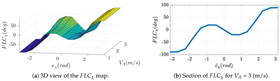
Figure 7.
Input-Output map of the Fuzzy system .
3. Rendezvous and Pursuit with a Moving Target
3.1. Vehicle-Target Relative Kinematics
The position error dynamics can be obtained by defining and differentiating the vehicle-target relative position equation. Given the position of the vehicle and that of target in the earth reference system, the position error vector is:
and its derivative is:
It should be noted that the fuzzy maps are defined in the waypoint reference frame, thus it is necessary to study the position error dynamics in the waypoint frame; this, as will be made evident later, is especially important when the target is moving and the waypoint frame is rotating. Starting from Equation (1):
and differentiating yields:
Equation (14) represents the kinematics of the relative position of aircraft and target in the waypoint frame.
3.2. Pursue of Waypoints and Static Targets
When the target is not moving and the waypoint frame has a constant orientation, Equation (14) reduces to:
and the position error dynamics depend on the aircraft velocity vector only. The rationale behind the proposed fuzzy guidance system is that by choosing the velocity vector (rotated into waypoint frame) to be always aligned with the desired approach direction described by the maps in Figure 4 and Figure 6, the vehicle will be ultimately guided at the target arriving from the desired approach direction. Since the vector can be expressed in polar coordinates as: where and , aircraft speed and heading can be set independently according to the FGS output. As a result, when the target is not moving () and the waypoint frame is not rotating (), when is set to the desired waypoint crossing speed and is obtained from the fuzzy maps, the position error will go towards zero following the paths represented by the arrows in Figure 4 and Figure 6.
Only for exemplification, Figure 8a shows sample trajectories obtainable with the proposed FGS with a static target (or waypoint) at the center of the image and various desired crossing directions; the FGS generates smooth trajectories that bring the vehicle to the target aligned with the desired approach direction represented in the figure with an arrow of the same trajectory color. Figure 8b instead shows some trajectories generated by changing the vehicle’s initial position: 18 different initial positions were placed at a distance of 5 m from the target, the initial vehicle heading was set pointing toward the top of the figure for all initial positions. The FGS generates smooth trajectories that have the vehicle align first with the fuzzy map and to “follow the arrows” of Figure 4 and Figure 6 to reach the target correctly aligned.
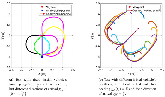
Figure 8.
Simulation of FGS towards a static target with different initial and final conditions.
3.3. Pursue of Targets Moving in Rectilinear Motion
When the target to be reached is moving in rectilinear motion with constant velocity and the waypoint frame is not rotating, Equation (14) decreases to:
that shows how the error dynamics depend on aircraft-target relative velocity. It has been shown [29] that the intercept performance of the proposed FGS degrades rapidly as a function of the target speed ; the solution proposed in [29] for the case of constant target velocity vector, that will be briefly recalled in the following, was to define a virtual vehicle with position such that at initial time , to define the virtual vehicle velocity as:
and to note that the rate of change of position error coincides with the virtual vehicle velocity , that is:
Thus, the desired FGS performance can be achieved with targets moving in rectilinear motion by defining the virtual vehicle heading and speed :
with:
and by regulating them, instead of those of the real vehicle, to the output of the guidance system. In addition, in order to intercept the target with the desired relative speed , the magnitude of the virtual vehicle’s velocity, that is the relative speed, must be kept equal to , that is:
Squaring both sides and replacing the expression of the vehicle and target velocities:
yields the desired vehicle speed :
Furthermore, in order to intercept the target with , a different desired heading angle at the waypoint is introduced: . When the real vehicle reaches the waypoint with the correct speed and the correct heading angle , the virtual vehicle speed is:
Thus, the virtual vehicle heading angle, when crossing the initial waypoint/target position must be:
that is, in other words, is the direction that the relative velocity vector must have so that the aircraft velocity vector is aligned with . It can be easily shown that when . Finally, the FGS output, that is the reference heading for the autopilot, becomes:
where is the output of the first stage of the heading controller:
the term is the heading error for the second stage of the heading controller, the term compensates for the difference between the directions of the velocity vectors of the virtual and the real aircraft, and are the velocity-compensated position errors along the waypoint frame X and Y axes:
It is easy to show that when the virtual vehicle velocity vector is aligned with , the aircraft velocity vector is aligned with in Equation (26).
3.4. Pursue of Accelerating Targets
If the target is accelerating, the direction and length of the velocity vector change in time. Equation (16) still holds and, assuming that velocity and acceleration of the target can be measured, the solution proposed above still works. A target that accelerates varies its velocity vector and, in turns, with the acceleration normal to the trajectory path, its velocity vector rotates with a certain angular velocity. This let us introduce a more interesting case, also in relation to a solution to the rendezvous problem described subsequently: the case of rotating waypoint frame.
Although in principle and in the most general case, the waypoint frame may be rotated arbitrarily (i.e., is not constant and varies arbitrarily), keeping in mind that the waypoint desired approach direction is set by the user of the FGS, the only scenarios of practical usefulness are those in which the desired approach path to a target is somehow related to the direction of the velocity vector of the target itself. Rendezvous is one of these: approaching a moving target with desired relative velocity equal to zero at the “intercept” point can be achieved only by aligning first the velocity vectors and then by regulating the relative distance and velocity to zero. In order to obtain this, the approach path must arrive to the target from a direction that is always aligned with its velocity vector.
Such a case can be easily modeled in the framework of the proposed FGS by letting the waypoint frame to rotate with the target velocity that is by setting in (14) obtaining:
where the time derivative of the rotation matrix can be substituted with its equivalent form [32]:
obtaining:
where is a skew symmetric matrix of the following form:
and is the angular velocity of the target’s velocity vector. Equation (31) contains an additional term with respect to Equation (16) that sums up with target and vehicle velocities:
The additional velocity term can be considered the “transport” velocity induced by rotation of the waypoint frame. It is possible then to define the apparent velocity of the target:
that can be used to define the velocity of the virtual vehicle similarly to Equation (17):
This allows, considering the new definition of virtual vehicle velocity, one to reduce Equation (29) to:
Thus, the FGS with a maneuvering target and rotating waypoint frame can be modified similarly to the previous Section 3.3, but now using the virtual vehicle heading and speed :
With:
In addition, in order to intercept the target with the desired relative speed , the magnitude of the virtual vehicle’s speed must be kept equal to , that is:
consequently, the desired vehicle velocity is:
Similarly as above, imposing the intercept condition with allows one to compute the new desired rotation angle for the waypoint frame; when the real vehicle reaches the target with the correct speed and the correct heading angle , the virtual vehicle speed is:
Thus, the virtual vehicle heading angle, when crossing the waypoint/target position, must be:
Note that when the vehicle actually reaches the target, the transport term nulls and that implies, as should be expected, that .
To conclude, the FGS output, that is the reference heading for the autopilot, in case of accelerating target and rotating waypoint frame, becomes:
where is the output of the first stage of the heading controller:
the term is the heading error for the second stage of the heading controller, the term compensates for the difference between the directions of the velocity vectors of the virtual and the real aircraft, and are the speed-compensated position errors along the waypoint frame X and Y axes:
A final remark is now opportune. The term represents a “transport” velocity term that is large when the vehicle is far from the target and can also become large if the waypoint frame is rotating very quickly, that happens when the target accelerates robustly, but anyway becomes smaller as the aircraft approaches the waypoint (since ). In most practical situations, it is likely that the term is always much smaller than the other two velocity terms in Equation (31), thus it could be confidently neglected, especially if the angular velocity is unknown or difficult to measure. Furthermore, also for the rendezvous case that will be presented in Section 3.5, this term can be neglected, since the rendezvous point of interest is likely to be at, or very close to, the target, so that the .
If and are computed without considering the term , that is using in the place of , then the rotation of the waypoint frame appears as an input disturbance to the FGS. However, the effect of such disturbance may not be destabilizing, as can be seen by studying the error dynamics with only the disturbance term present:
that is:
It can be easily seen by inspection that the trajectories of arising, for instance, from a constant non-null angular velocity are circles centered at the origin of the waypoint frame and passing from the current position of the vehicle. When this disturbance is applied to the vehicle controlled by the FGS, it has an effect similar to the warping of the fuzzy maps in Figure 4 and Figure 6, but, as long as the commanded velocity resulting from the FGS and the disturbance reduces the distance from the waypoint, the generated trajectories, though deformed, will tend toward the waypoint. Thus, as long as the disturbance is not too large, the FGS will be able to reject it in closed loop. When the disturbance is too large, as for instance, when the transport velocity amplitude becomes similar to the speed of the aircraft, the vehicle will likely start orbiting around the waypoint failing to reach it, as could be easily shown in simulation. These limit cases are anyway of little practical usefulness and are not discussed in detail here.
3.5. Rendezvous with a Moving Target
The FGS presented in the previous sections allows the vehicle to pursue and intercept fixed and mobile targets from any arrival angle. As discussed in the previous section, rendezvous with a target requires instead the alignment of aircraft and target velocity vectors; thus, the proposed FGS can be used effectively in this context by setting the desired direction of crossing to coincide and vary continuously with the direction of the target’s velocity vector . Since the proposed FGS generates trajectories that approach the target from behind, that is, that circulate around the target in order to arrive to it with the aircraft velocity vector aligned with the desired crossing direction (i.e., with ), when the aircraft is on the final part of the approach path (namely on the positive Y axis), the clear result is that the aircraft and target velocity vectors become aligned: .
From a practical point of view, successful rendezvous is achieved when the follower vehicle has reached a desired distance from the target and is able to keep it constant. Since the described guidance law is able to bring the vehicle to the interception of the target, but is not able to keep it at constant distance, a modification is necessary to adjust the relative speed when close enough to the desired rendezvous point.
With the proposed FGS, a rendezvous maneuver can be divided in three phases:
- Braking phase (BP): braking starts when the vehicle is behind the target within a certain error interval expressed in waypoint coordinates. The required speed is linearly reduced down to the target speed . This behaviour is useful to avoid undesirable overshoot on the axis. Only the speed controller is involved in this phase, the heading controller is unaffected;
- Formation keeping phase (FKP): Formation keeping starts when the vehicle has queued up and is close to the final rendezvous position. Within the formation keeping phase, dynamic controllers are activated to keep the pursuer at the desired position. Two decoupled position controllers are used to keep the aircraft at the desired point : the first controller corrects the desired reference speed as a function of and has as feedforward term, and the second one controls lateral displacement to .
According to the above subdivision into phases of the entire maneuver, the FGS described by Equations (3) and (4) is augmented to obtain the general form of the rendezvous fuzzy guidance system (rendezvous-FGS):
and
where the parameters and are defined as:
The parameter is used to control the interval within which the vehicle speed is linearly decreased; the term is the distance from the target, along the axis, where the vehicle starts decelerating, and is used to implement the braking phase by smoothly blending the FGS required speed (used in the pursuit phase) with the “final” desired speed: the target speed .
The parameter instead can be considered a Boolean flag that indicates if the braking and formation keeping phases can be activated or not: if the aircraft is pursuing the target from behind and lateral error is small, that is the vehicle is correctly aligned with the waypoint desired crossing direction, then the rendezvous phase can take place. When this condition is not met, either before actually starting the braking or formation keeping phases, or during one of these two, the rendezvous maneuver is aborted, the FGS takes over and another attempt is performed. The positive value specifies a sufficiently small lateral distance under which the maneuver can be considered safe.
The terms and introduced in Equations (48) and (49) represent additional control actions that regulate the aircraft position to the desired rendezvous point and could be implemented, in principle, with any controller structure. In the present work, these have been implemented as PID controllers:
and
Equations (48)–(51) constitute the general representation of the rendezvous-FGS, however, in order to avoid frequent, unwanted and unnecessary transitions between phases, a hysteresis function was applied to the testing of the sign of the parameter . Looking at Figure 9, when the vehicle enters the braking phase, the value of decreases from 1 to 0 as it moves closer to the desired distance . Using in place of when testing the sign of it in Equations (48) and (49) guarantees that the formation keeping phase starts when and is not deactivated unless (i.e., it exceeds a given positive threshold). Thus, the hysteresis prevents possible unwanted transitions between the braking and the formation keeping phases when the aircraft oscillates around the desired rendezvous point. This allows the formation keeping controllers to operate more effectively.
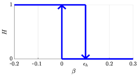
Figure 9.
Hysteresis function on parameter ; it avoids chattering transitions between BP and FKP.
3.6. Rendezvous Simulation Results
In order to demonstrate the rendezvous capabilities of the proposed FGS, three scenarios were simulated: rendezvous with a target in linear motion at constant velocity, rendezvous with a uniformly accelerating target moving in circular motion, and a more challenging rendezvous situation with a target that performs instantaneous changes of acceleration, both in amplitude and sign, simulating a series of escape maneuvers.
The simulations were designed to resemble outdoor situations where a pursuer aircraft is guided initially in the vicinity of its target at a distance where it is possible to detect it with the onboard sensors, like, for instance a 3D camera similar to the approach described in [33], or other specific sensors like in [8]. At this distance, around 10 m, the FGS can be activated, since the relative motion (position and velocity) with respect to the target can be measured or estimated. The problem of pursuing the target from larger distances to bring the vehicle close enough so that the FGS can operate can be faced with various techniques and have been already treated, for instance, in [29], thus is not taken into consideration here.
The results shown are obtained with a very simple dynamic model of multi-rotor aircraft and are presented here only for the purpose of giving clear evidence of the FGS functioning; experimental results are shown in the Section 4.
3.6.1. Linear Motion Rendezvous
In this simulation, the target is initially placed 5 m in front of the pursuer aircraft and headed approximately to its right moving at 1 m/s. Desired rendezvous point is 1 m behind the target. The initial aircraft heading is . The FGS is activated and the resulting trajectory is shown in Figure 10a. Figure 10b shows the position of the pursuer aircraft in waypoint coordinates; it can be clearly seen that lateral error goes to zero quicker than the longitudinal error, indicating a correct approach path during the pursuit phase; then, the vehicle proceeds toward the intercept point, the braking phase starts, and later on, the formation keeping phase is entered and never exited until the end of the simulation.
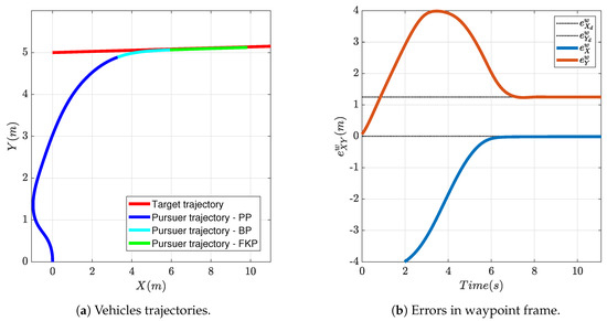
Figure 10.
Rendezvous example: the target moves with uniform rectilinear motion.
3.6.2. Circular Motion Rendezvous
In this second simulation, the target is placed approximately 10 m in front of the pursuer aircraft and engages a counterclockwise circular motion with a radius of 10 m. Desired rendezvous point is 1 m behind the target. The initial aircraft heading is . The FGS is activated and the resulting trajectory is shown in Figure 11a. Figure 11b shows the position of the pursuer aircraft in waypoint coordinates; similarly to the previous simulation, the three phases are stepped one after the other until the rendezvous point is reached and never left.
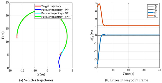
Figure 11.
Rendezvous example: the target is accelerating and moves with uniform circular motion.
3.6.3. Escaping Target Rendezvous
In this third simulation, the target is placed approximately 7 m behind and at the right of the pursuer aircraft, where in reality it could not be seen by the pursuer, and engages a sequence of 4 successive turns with increasing lateral acceleration. The desired rendezvous point is 1.25 m behind the target. The initial aircraft heading is . The FGS is activated and the resulting trajectory is shown in Figure 12a. Figure 12b shows the position of the pursuer aircraft in waypoint coordinates. Similarly to the other two simulations, the rendezvous-FGS is capable of bringing the aircraft to the rendezvous point and of keeping it close to it, even when the target changes instantaneously its acceleration and turn direction; short and little error transients, though, can be noticed when the target changes direction and acceleration. Figure 13 shows the position error in the waypoint frame as a map view to highlight that the system is capable of achieving and maintaining the rendezvous point with a very small error.
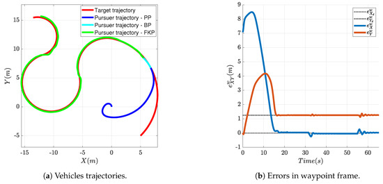
Figure 12.
Rendezvous example: the target is escaping and changes its angular velocity during the motion.
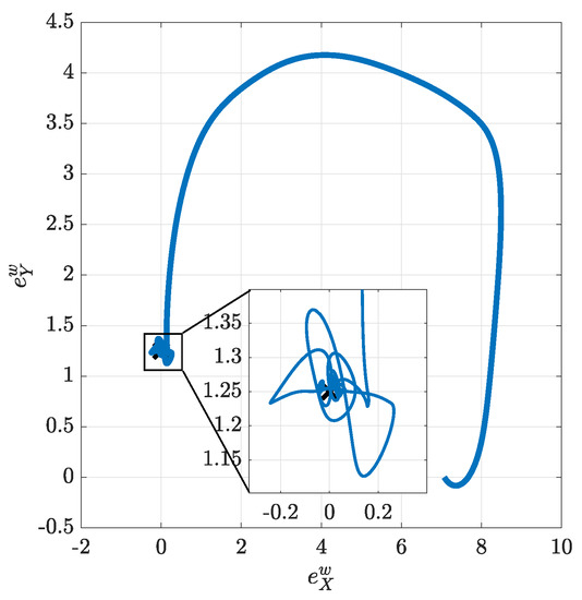
Figure 13.
Rendezvous example: escaping target—Map view of error in waypoint coordinates.
3.6.4. External Disturbances
Although external disturbances were not considered explicitly in the FGS design phase, and the proposed FGS is not designed explicitly for disturbance rejection, simulations have shown that it can stand significantly large velocity disturbances. The following shows the results of a simulation with the same initial conditions of the linear motion rendezvous example presented above, where a constant wind disturbance m/s, that is 25% of target velocity, is applied. Figure 14a shows the map view of this simulation: wind initially pushes the pursuer from the back that, after having aligned with the target velocity vector, receives the wind from its right side; in order to fly with such sidewind, the aircraft must turn its nose into the wind with the necessary sideslip angle. It can be seen that the pursuer successfully executes the PP, BP and FKP phases, even if some oscillations may be noticed. Figure 14c shows that, as expected, the desired heading produced by the FGS converges to the target velocity vector angle , since the pursuer is at the right position in the fuzzy map. Furthermore, the aircraft turns its nose to the right: the aircraft heading converges to the desired heading . Thus, thanks to the contribution of the rendezvous controller, the position error converges to 0 (Figure 14b). It should be noticed that the FGS successfully brought the aircraft close to the rendezvous point even without the presence of the term (during PP and BP phases), showing a certain robustness to external disturbances. Additionally, should an estimate of wind disturbance be available, like for instance the one presented in [17], this could be used to implement a direct wind compensation during the entire flight.
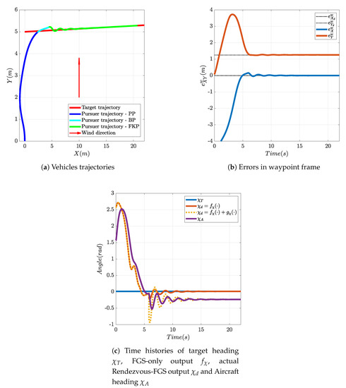
Figure 14.
Rendezvous with a moving target in presence of lateral wind = 0.25 (m/s).
Anyway, since similar results can be obtained for the other two sample rendezvous experiments, it could be argued that the proposed system should achieve successful rendezvous, as long as the FGS can bring the aircraft close enough to the right spot for the beginning of the FKP phase. Nonetheless, a more detailed analysis is outside the scope of this paper and will be subject of future studies.
4. Experimental Results
This section presents the experimental validation of the proposed rendezvous-FGS for both static and moving targets. The experiments were conducted in the indoor flight room of the LARS laboratory at the Dipartimento di Ingegneria dell’Informazione (DII) of the University of Pisa. The flight room is a suitable environment for conducting tests in complete safety, but the available flight volume does not allow the large maneuvers conducted in the simulations shown previously. Thus, the FGS was slightly modified to generate trajectories with a much smaller turn radius, but which were still achievable by a multi-rotor aircraft. The test was conducted using the multi-rotor aircraft in Figure 15; the vehicle is made up of a commercial drone frame (Tarot 650 Sport), a single board computer (SBC) (a NVIDIA Jetson TX2 was used for the experiments presented in this paper) and a custom autopilot system named ICARO III that uses a STM32F4 microcontroller—the hardware and firmware have been developed and maintained over the last 10 years in our laboratory at University of Pisa [34]. The flight room is equipped with a Vicon motion capture system that is used to measure the position of the vehicle, since GPS cannot be used. The position estimated by the Vicon system was used to provide simulated GPS fixes to the inertial navigation system of the ICARO III autopilot: a 16-state extended Kalman filter (EKF) that estimates vehicle attitude (using quaternions), position, velocity and acceleration using a 9-axis IMU (3 gyroscopes, 3 accelerometers and 3 magnetometers—MPU6050 and HMC5883), a barometric altimeter (BMP85), an ultrasonic altimeter (for low altitude, less than 5 m, flight—MaxSonar), and GPS (simulated in this case). The ICARO III Autopilot runs inner control loops (roll, pitch and yaw angles regulation) at 200 Hz, while the EKF and outer loop velocity and position control algorithms run at 50 Hz; concurrency and determinism is guaranteed by the use of the FreeRTOS real-time operating system. The SBC, that runs Linux and uses the robotic operating system (ROS) for inter-process communications, takes care of high-level mission management and runs all computationally intensive non-real-time algorithms, like, for instance, the vision algorithms described in [33], and, additionally, takes care of interfacing with the VICON system to send simulated GPS data to the autopilot using a serial link. Given the small available flight volume, the size of vehicle (about 0.8 m tip to tip), and in order to avoid risk of collision, the target to be pursued in all these experiments is a virtual vehicle that is moving inside the airspace of the flight room. The perception system of the pursuer aircraft is simulated inside the SBC and relative position and velocity estimates are provided to the autopilot that implements the FGS.
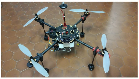
Figure 15.
The vehicle used for the experimental validation.
4.1. Fixed Targets
In order to test the FGS scaled down to generate trajectories flyable indoor, some preliminary experiments were conducted with fixed virtual targets positioned at the center of the flight volume. Figure 16 shows the trajectories obtained during three tests conducted in this configuration. The three tests differ only in the desired arrival direction .
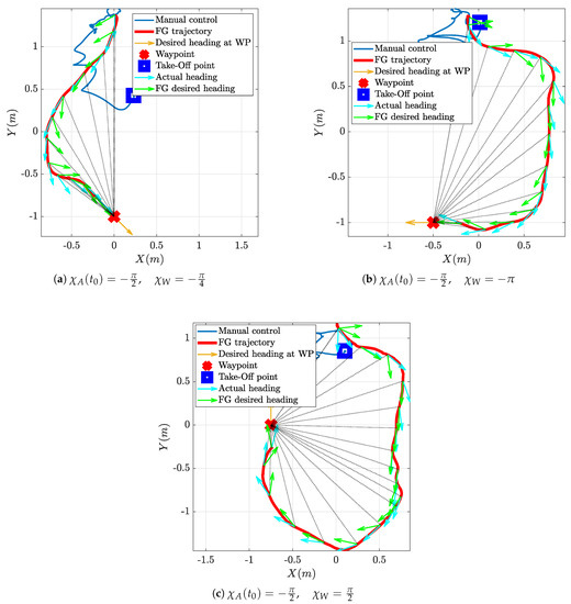
Figure 16.
Experimental test of FGS for a static target and different final directions of arrival .
The flight starts with manual piloting with the take-off, then the drone is driven automatically to the selected initial position m, where it loiters and aligns its yaw angle , using the position control algorithm available onboard ICARO, until the FGS is activated; at this point, the FGS takes control and the desired heading and speed are used as reference values for the attitude and velocity controllers onboard the ICARO autopilot.
The three Figure 16 show the trajectory conducted under FGS guidance in solid red, the vehicle’s heading along the trajectory as cyan arrows and the desired heading as green arrows; the desired heading at the waypoint, that is the desired arrival direction, is shown as a yellow arrow placed at the waypoint position (the red cross mark). The thin dotted black lines represent the line-of-sight-vector between the aircraft and its target. The experimental results show that the FGS is able to guide the vehicle towards the target starting from different initial conditions (in the waypoint reference frame). The FGS allows the vehicle to reach the target with the desired orientation, either starting from behind or starting from the side, as well as face to face. The trajectories obtained are very close to the ones obtained in simulation and shown in Figure 8a and follow those produced by the fuzzy maps in Figure 4 and Figure 6, even if they appear scaled since the FGS map was resized to fit in the available flight volume.
In all three experiments, it can also be noted that the aircraft heading appears to align slowly to the desired heading (the cyan arrows appear to follow the green arrows with a certain lag), resulting in a slightly deformed trajectory with respect to the simulations, yet not preventing the successful reach of the waypoint from the desired direction and with the desired orientation. This is due to the dynamics of the yaw controller onboard ICARO; this controller was tuned for outdoor operations and the maximum turn rate is intentionally kept low in order to prevent possible problems under position control and with wind gusts. It must also be considered that, unfortunately, the vehicle size is comparable with the breadth of the entire trajectory, also the desired speed is very low compared to the vehicle capabilities, thus these trajectories appear very tight and challenging for it. Even if other smaller vehicles are available in the laboratory for indoor only use, we preferred to use the larger vehicle, since it features a complete GPS-INS navigation system and onboard vision processing capabilities (via a NVIDIA Jetson TX2) that will enable future outdoor experiments using the system described in [33].
4.2. Rendezvous with an Accelerating Target
Due to space limitations, it was not possible to implement experiments with targets in rectilinear motion. Thus, only one experiment with an accelerating target is presented. This experiment aims at testing the FGS in a realistic situation similar to that shown in Figure 11.
Figure 17a shows the trajectory produced by the vehicle during the pursuing of an accelerating virtual target; the target performed a narrow circular uniform motion (thick black dotted line) with = 0.2 m/s and turn radius m. The flight starts with manual piloting with the take-off, then the drone is driven manually to a suitable starting position facing the target to be pursued, then the virtual vehicle motion is started and the FGS is activated. The thin dotted black lines represent the line-of-sight-vector between the aircraft and its target and are drawn to help visualize the relative position between the two vehicles at various points in time.
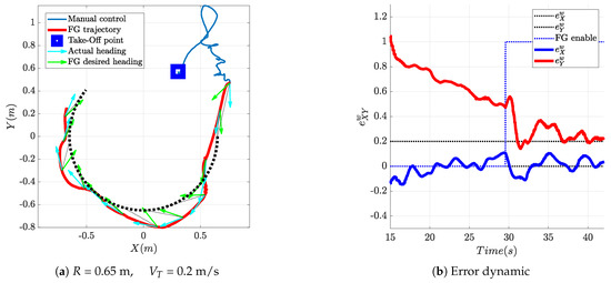
Figure 17.
FGS experimental test: the target is accelerating and moves with uniform circular motion.
The aircraft was able to follow the target in its uniform circular motion, even if the trajectory is not as good as that obtained in simulation (Figure 11). Nonetheless, the tracking error, the relative position in waypoint coordinates between the aircraft and the desired rendezvous point, as shown in Figure 17b, converges to the desired value m. The residual oscillations around the rendezvous point, for a maximum error of around 10 cm, are mainly due to yaw controller dynamics and to the fact that the onboard velocity controller, that tracks the reference velocity produced by the FGS, was designed for much larger velocities and has difficulties in regulating the vehicle speed to the desired m/s. The tendency to stay outside of the target trajectory is expected, since the chaser vehicle should stay 20 cm behind the target along the tangent to its trajectory, oscillations are anyway due to the dynamics of the yaw controller; as a matter of fact, a similar result can also be obtained in simulation by introducing the flight control system dynamics. In order to make it more readable, Figure 17 shows just the first portion of the vehicles’ trajectories recorded during the experiment. Figure 18 shows instead the full trajectory of the experiment in which target and pursuer performed three entire circles. It can be easily seen that the FGS can successfully bring the vehicle onto the target trajectory and keep it close to the desired rendezvous point.
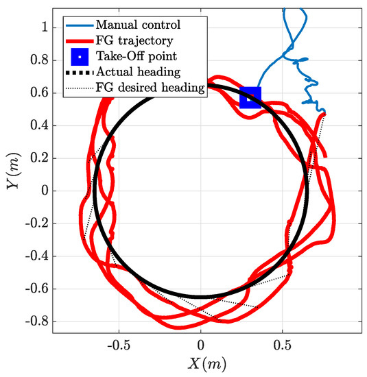
Figure 18.
FGS experimental test: the target moves with uniform circular motion—full trajectory.
5. Conclusions
This paper has presented a fuzzy guidance system capable of pursuing moving targets as an extension to a previous work of the same authors introducing and discussing in detail the case of pursuing an accelerating target, and of time-varying desired target crossing direction. In addition, it presented the novel rendezvous-fuzzy guidance system, capable not only of pursuing a target, but also of performing rendezvous maneuvers with accelerating targets. Simulations were presented to support the mathematical results, and finally an experimental validation is proposed where a multi-rotor vehicle is brought to intercept virtual targets in a controlled indoor environment. The experimental results have confirmed the capability of the proposed fuzzy guidance system to intercept or rendezvous with both fixed and moving targets.
Author Contributions
Conceptualization, M.I. and L.P.; Funding acquisition, L.P.; Writing—original draft, M.A.; Writing—review & editing, L.P. All authors have read and agreed to the published version of the manuscript.
Funding
This research received no external funding.
Acknowledgments
The authors would like to thank Valeria Sarno and Alessandro Procopio, students of the Master’s Degree of Robotics and Automation Engineering of University of Pisa, for their support in preparing the preliminary experiments of the FGS presented in this paper. The authors would also like to thank Andrea Berton, director of ReFly (Research in Fly) of CNR Italy, for providing the vehicle used in the experiments.
Conflicts of Interest
The authors declare no conflict of interest.
Abbreviations
The following abbreviations are used in this manuscript:
| FGS | Fuzzy Guidance System |
| TS | Takagi–Sugeno |
| FLC | Fuzzy Logic Controller |
| MF | Membership Function |
| SBC | Single Board Computer |
| GPS | Global Positioning System |
| IMU | Inertial Measurement Unit |
| INS | Inertial Navigation System |
References
- Zarchan, P. Tactical and Strategic Missile Guidance; American Institute of Aeronautics and Astronautics, Inc.: Reston, VA, USA, 2012. [Google Scholar]
- Fehse, W. Automated Rendezvous and Docking of Spacecraft; Cambridge Aerospace Series; Cambridge University Press: Cambridge, UK, 2003. [Google Scholar] [CrossRef]
- Teo, K.; Goh, B.; Chai, O.K. Fuzzy docking guidance using augmented navigation system on an AUV. IEEE J. Ocean. Eng. 2014, 40, 349–361. [Google Scholar] [CrossRef]
- Allibert, G.; Hua, M.D.; Krupínski, S.; Hamel, T. Pipeline following by visual servoing for Autonomous Underwater Vehicles. Control. Eng. Pract. 2019, 82, 151–160. [Google Scholar] [CrossRef]
- Jacobi, M. Autonomous inspection of underwater structures. Robot. Auton. Syst. 2015, 67, 80–86. [Google Scholar] [CrossRef]
- Wu, H.M.; Karkoub, M.; Hwang, C.L. Mixed fuzzy sliding-mode tracking with backstepping formation control for multi-nonholonomic mobile robots subject to uncertainties. J. Intell. Robot. Syst. 2015, 79, 73–86. [Google Scholar] [CrossRef]
- Kosari, A.; Jahanshahi, H.; Razavi, S. An optimal fuzzy PID control approach for docking maneuver of two spacecraft: Orientational motion. Eng. Sci. Technol. Int. J. 2017, 20, 293–309. [Google Scholar] [CrossRef]
- Klionovska, K.; Ventura, J.; Benninghoff, H.; Huber, F. Close Range Tracking of an Uncooperative Target in a Sequence of Photonic Mixer Device (PMD) Images. Robotics 2018, 7, 5. [Google Scholar] [CrossRef]
- Kluever, C.A. Feedback Control for Spacecraft Rendezvous and Docking. J. Guid. Control. Dyn. 1999, 22, 609–611. [Google Scholar] [CrossRef]
- Carter, T.E. State Transition Matrices for Terminal Rendezvous Studies: Brief Survey and New Example. J. Guid. Control. Dyn. 1998, 21, 148–155. [Google Scholar] [CrossRef]
- Zeng, Z.; Sammut, K.; Lian, L.; Lammas, A.; He, F.; Tang, Y. Rendezvous Path Planning for Multiple Autonomous Marine Vehicles. IEEE J. Ocean. Eng. 2018, 43, 640–664. [Google Scholar] [CrossRef]
- Papen, A.; Vandenhoeck, R.; Bolting, J.; Defay, F. Collision-Free Rendezvous Maneuvers for Formations of Unmanned Aerial Vehicles. IFAC-PapersOnLine 2017, 50, 282–289. [Google Scholar] [CrossRef]
- Smith, A.L. Proportional Navigation with Adaptive Terminal Guidance for Aircraft Rendezvous. J. Guid. Control. Dyn. 2008, 31, 1832–1836. [Google Scholar] [CrossRef]
- Ochi, Y.; Kominami, T. Flight Control for Automatic Aerial Refueling via PNG and LOS Angle Control. In Proceedings of the AIAA Guidance, Navigation, and Control Conference and Exhibit, San Francisco, CA, USA, 15–18 August 2005. [Google Scholar] [CrossRef]
- Vaneck, T. Fuzzy guidance controller for an autonomous boat. IEEE Control. Syst. Mag. 1997, 17, 43–51. [Google Scholar]
- Rae, G.; Smith, S. A fuzzy rule based docking procedure for autonomous underwater vehicles. In Proceedings of the OCEANS 92 Proceedings@ m_Mastering the Oceans Through Technology, Newport, RI, USA, 26–29 October 1992; Volume 2, pp. 539–546. [Google Scholar]
- Teo, K.; An, E.; Beaujean, P.P.J. A robust fuzzy autonomous underwater vehicle (AUV) docking approach for unknown current disturbances. IEEE J. Ocean. Eng. 2012, 37, 143–155. [Google Scholar] [CrossRef]
- Pearson, D.; An, E.; Dhanak, M.; von Ellenrieder, K.; Beaujean, P. High-level fuzzy logic guidance system for an unmanned surface vehicle (USV) tasked to perform autonomous launch and recovery (ALR) of an autonomous underwater vehicle (AUV). In Proceedings of the 2014 IEEE/OES Autonomous Underwater Vehicles (AUV), Oxford, MS, USA, 6–9 October 2014; pp. 1–15. [Google Scholar] [CrossRef]
- Xiang, X.; Yu, C.; Lapierre, L.; Zhang, J.; Zhang, Q. Survey on fuzzy-logic-based guidance and control of marine surface vehicles and underwater vehicles. Int. J. Fuzzy Syst. 2018, 20, 572–586. [Google Scholar] [CrossRef]
- Li, H.; He, S.; Wang, J.; Shin, H.S.; Tsourdos, A. Near-Optimal Midcourse Guidance for Velocity Maximization with Constrained Arrival Angle. J. Guid. Control. Dyn. 2021, 44, 172–180. [Google Scholar] [CrossRef]
- Ratnoo, A.; Ghose, D. Impact Angle Constrained Interception of Stationary Targets. J. Guid. Control. Dyn. 2008, 31, 1817–1822. [Google Scholar] [CrossRef]
- Kumar, S.R.; Rao, S.; Ghose, D. Nonsingular Terminal Sliding Mode Guidance with Impact Angle Constraints. J. Guid. Control. Dyn. 2014, 37, 1114–1130. [Google Scholar] [CrossRef]
- Nakai, K.; Uchiyama, K. Vector Fields for UAV Guidance Using Potential Function Method for Formation Flight. In Proceedings of the AIAA Guidance, Navigation, and Control (GNC) Conference, Boston, MA, USA, 19–22 August 2013. [Google Scholar] [CrossRef]
- Nelson, D.R.; Barber, D.B.; McLain, T.W.; Beard, R.W. Vector field path following for small unmanned air vehicles. In Proceedings of the 2006 American Control Conference, Minneapolis, MN, USA, 14–16 June 2006. [Google Scholar] [CrossRef]
- Pakpong, J.; Wilson, P.A. Control and guidance for homing and docking tasks using an autonomous underwater vehicle. In Proceedings of the 2007 IEEE/RSJ International Conference on Intelligent Robots and Systems, San Diego, CA, USA, 29 October–2 November 2007; pp. 3672–3677. [Google Scholar] [CrossRef]
- Frew, E.; Lawrence, D. Cooperative stand-off tracking of moving targets by a team of autonomous aircraft. In Proceedings of the AIAA Guidance, Navigation, and Control Conference and Exhibit, San Francisco, CA, USA, 15–18 August 2005; p. 6363. [Google Scholar]
- Lawrence, D.; Frew, E.; Pisano, W. Lyapunov vector fields for autonomous UAV flight control. In Proceedings of the AIAA Guidance, Navigation and Control Conference and Exhibit, Hilton Head, CA, USA, 20–23 August 2007; p. 6317. [Google Scholar]
- Hough, J.G.; Ulrich, S. Lyapunov Vector Fields for Thrust-Limited Spacecraft Docking with an Elliptically-Orbiting Uncooperative Tumbling Target. In Proceedings of the AIAA Scitech 2020 Forum, Orlando, FL, USA, 6–10 January 2020; p. 2078. [Google Scholar]
- Innocenti, M.; Pollini, L.; Turra, D. A fuzzy approach to the guidance of unmanned air vehicles tracking moving targets. IEEE Trans. Control. Syst. Technol. 2008, 16, 1125–1137. [Google Scholar] [CrossRef]
- Takagi, T.; Sugeno, M. Fuzzy identification of systems and its applications to modeling and control. IEEE Trans. Syst. Man, Cybern. 1985, SMC-15, 116–132. [Google Scholar] [CrossRef]
- Tanaka, K.; Ikeda, T. Stability analysis of feedback systems in fuzzy phase-lead compensation. In Proceedings of the 1995 IEEE International Conference on Systems, Man and Cybernetics. Intelligent Systems for the 21st Century, Vancouver, BC, Canada, 22–25 October 1995; Volume 3, pp. 2165–2170. [Google Scholar]
- Rogers, R.M. Applied Mathematics in Integrated Navigation Systems; American Institute of Aeronautics and Astronautics: Reston, VA, USA, 2007. [Google Scholar]
- Esposito, N.; Fontana, U.; D’autilia, G.; Bianchi, L.; Alibani, M.; Pollini, L. A Hybrid Approach to Detection and Tracking of Unmanned Aerial Vehicles. In Proceedings of the AIAA Scitech 2020 Forum, Orlando, FL, USA, 6–10 January 2020. [Google Scholar] [CrossRef]
- Pollini, L.; Innocenti, M.; Di Corato, F.; Cellini, M.; Franchi, M.; Mati, R.; Niccolai, V. The ICARO Autopilot: A flexible Controller for Small Unmanned Air Vehicles. Available online: https://arpi.unipi.it/handle/11568/134170#.X91t7RapTIU (accessed on 19 December 2020).


Publisher’s Note: MDPI stays neutral with regard to jurisdictional claims in published maps and institutional affiliations. |
© 2020 by the authors. Licensee MDPI, Basel, Switzerland. This article is an open access article distributed under the terms and conditions of the Creative Commons Attribution (CC BY) license (http://creativecommons.org/licenses/by/4.0/).