LIDAR Scan Matching in Off-Road Environments

Abstract

Accurately matching the LIDAR scans is a critical step for an Autonomous Land Vehicle (ALV). Whilst most previous works have focused on the urban environment, this paper focuses on the off-road environment. Due to the lack of a publicly available dataset for algorithm comparison, a dataset containing LIDAR pairs with varying amounts of offsets in off-road environments is firstly constructed. Several popular scan matching approaches are then evaluated using this dataset. Results indicate that global approaches, such as Correlative Scan Matching (CSM), perform best on large offset datasets, whilst local scan matching approaches perform better on small offset datasets. To combine the merits of both approaches, a two-stage fusion algorithm is designed. In the first stage, several transformation candidates are sampled from the score map of the CSM algorithm. Local scan matching approaches then start from these transformation candidates to obtain the final results. Four performance indicators are also designed to select the best transformation. Experiments on a real-world dataset prove the effectiveness of the proposed approach.

1. Introduction

Simultaneous Localization and Mapping (SLAM) has always been a hot research topic in the field of autonomous driving. One of the core modules behind SLAM is the ability to accurately register two scans captured in nearby positions. LIDAR is among the most popular sensors for an Autonomous Land Vehicle (ALV) due to its highly precise range measurements [1,2]. Whilst most of the previous works have focused on urban environments, this paper focuses on the problem of registering two LIDAR scans captured in an off-road environment.

There have been a lot of research on LIDAR point cloud registration, and many approaches have been proposed, such as Generalized-ICP (GICP) [3,4], Normal Distribution Transform (NDT) [5,6], LIDAR Odometry and Mapping (LOAM) [7], Correlative Scan Matching (CSM) [8], etc. However, those approaches are mostly designed for urban environments. In the off-road environment, some new challenges might be encountered:

• In off-road environments, the distribution of trees and bushes is random and cluttered, as shown in Figure 1. Therefore, the point’s curvature, normal and other geometric features, which are frequently used in existing approaches, are unstable. For example, GICP uses the plane-to-plane distance to describe the proximity of two matched points, which requires calculating the covariance matrix and the surface normal at that point. However, cluttered points will weaken these features and may cause mismatches. The edge point and planar point selected in the LOAM algorithm are also closely related to the point’s curvature, which may not be accurately estimated in the off-road environment.
• In off-road environments, the vehicle, as well as the LIDAR attached to it, might shake abruptly. This unexpected movement may change the local distribution of points. Consequently, the performance of NDT may be degraded, as this algorithm requires the distribution of local points to be stable.

In this paper, the problem of registering LIDAR scans in an off-road environment is investigated. The main contributions of this paper are as as follows:

• A dataset containing a large number of LIDAR pairs with different offsets in an off-road environment is proposed.
• A rigorous evaluation of existing scan matching approaches is performed on this dataset, and results indicate that CSM [8] performs best on large offset dataset, whilst LOAM performs better on small offset dataset.
• A more robust approach combining the advantages of CSM and LOAM is proposed. Experiments on the dataset indicate that the proposed method performs better than existing scan registration approaches.

2. Related Work

For matching two LIDAR scans, based on how they model the point cloud, existing methods could be categorized into local approaches and global approaches. Whilst local approaches treat the point cloud as an assembly of local segments, global approaches treat the point cloud as a whole.

For local approaches, it focuses on optimizing the distance between corresponding local geometric structures. Iterative Closet Point (ICP) algorithm and its variants [3,4,9] are the defacto baseline approaches for LIDAR point cloud matching. These approaches either use point-to-point, point-to-plane, or plane-to-plane distance as the proximity measure for two local geometric structures. Normal Distribution Transformation (NDT) [5,10] is another LIDAR scan matching approach which models the local geometric structure as a normal distribution. The distance between the local geometric structures is then computed using the mahalanobis distance. For faster iteration and more robust distance modeling, LOAM algorithm [7,11] only selects a subset of point clouds which are either the edge points or the planar points. For the edge points, the point-to-line distance was used, whilst the point-to-plane distance was used for the planar points.

For global approaches [12], the point cloud is considered as a whole. To make the computation tractable, it is often necessary to project the 3D point cloud to a 2D ground plane. In [13], the 3D LIDAR scan was projected onto a 2D orthographic reflectivity map. In [8], the Correlative Scan Matching (CSM) approach was used to match the two-point cloud in 2D. Similarly, a 2D height map is used to represent the 3D point cloud in [14,15]. Chong et al. [16] proposed a 2D map representation which combines reflectivity, height, color, curvature and normal for more robust matching. In [15], the authors utilized both the reflectance intensity map and the height map. The scan matching problem is casted as an optical flow [17] computation problem, and an efficient gradient descend approach is proposed to solve it.

Most of the methods mentioned above are designed and tested in urban environments. In this paper, the focus is on off-road environments. Three typical local scan matching methods: GICP, NDT, LOAM and a popular global method (CSM) will be tested in the following experiments.

3. Existing Scan Matching Approaches

The problem of scan matching is formally defined as follows. Let P and Q represent the target point cloud and the source point cloud respectively. These two-point clouds are then converted as $P^{\prime }=\mathcal{C}(P)$ and $Q^{\prime }=\mathcal{C}(Q)$ by some conversion function $\mathcal{C}$. The task of scan matching is to find a Euclidean transformation of $\mathcal{T}$ so that $\mathcal{T}(Q^{\prime })$ is best aligned with $P^{\prime }$. To improve readability, the superscript of the converted cloud is omitted in the following equations.

Possible forms of the conversion function $\mathcal{C}$ include: ${\mathcal{C}}_0$: a uniform downsampling of the original point cloud; ${\mathcal{C}}_1$: project the 3D point cloud to the ground plane to get 2D height map; ${\mathcal{C}}_2$: binarize the projected 2D height map to generate an obstacle map; ${\mathcal{C}}_3$: deletes those points that belong to the ground plane. A combination of different conversion functions is also possible, such as ${\mathcal{C}}_1+{\mathcal{C}}_2+{\mathcal{C}}_3$ or ${\mathcal{C}}_0+{\mathcal{C}}_3$, etc.

Let $q_i$ represent a point in the source point cloud, $p_i^{(\mathcal{G})}$ is its closest geometric structure in the target point cloud. The geometric structure can be points (spheres), lines or planes. In order to improve the robustness, a penalty function $\rho (•)$ is introduced to reduce the effect of outliers on optimization. The energy function of scan matching is usually expressed as:

$$E(\mathcal{T})=\sum \rho (\mathtt{dist}(p_i^{(\mathcal{G})},q_i^{(\mathcal{T})})).$$

(1)

3.1. The Generalized ICP (GICP) Approach

In this approach, it is assumed that each point is generated from its local distribution: $P=\{p_i\}$, $p_i\sim \mathcal{N}({\widehat{p}}_i,C_i^P)$ and $Q=\{q_i\}$, $q_i\sim \mathcal{N}({\widehat{q}}_i,C_i^Q)$, where ${\widehat{p}}_i$ and ${\widehat{q}}_i$ are the underlying ideal points (with no errors due to occlusion or sampling) s.t. ${\widehat{p}}_i={\mathcal{T}}^{\ast }({\widehat{q}}_i)$. $\{C_i^P\}$ and $\{C_i^Q\}$ are the covariance matrices associated with the local measurement points. Therefore, $p_i-{\mathcal{T}}^{\ast }(q_i)\sim \mathcal{N}(0,C_i^P+{\mathcal{T}}^{\ast }{C}_i^Q{\mathcal{T}}^{\ast }\mathsf{T})$. The distance function can be written as:

$${\mathtt{dist}}_{\mathtt{GICP}}={(p_i-q_i^{(\mathcal{T})})}^{\mathsf{T}}{(C_i^P+\mathcal{T}{C}_i^Q{\mathcal{T}}^{\mathsf{T}})}^{-1}(p_i-q_i^{(\mathcal{T})}).$$

(2)

The GICP algorithm treats the point cloud as a collection of many segmented planes. The term $C_i^P+\mathcal{T}{C}_i^Q{\mathcal{T}}^{\mathsf{T}}$ contains the covariance matrix of the two surfaces. When $C_i^P=\mathbf{I},C_i^Q=\mathbf{0}$, the above formula is equal to the point-to-point ICP. When $C_i^P={\mathbf{n}}_i\ast {\mathbf{n}}_i^T,C_i^Q=\mathbf{0}$, where ${\mathbf{n}}_i$ is the normal vector at $q_i$, the above equation is equivalent to point-to-plane ICP. When $C_i^P$ and $C_i^Q$ represent the covariance matrix at $p_i$ and $q_i$, GICP becomes the plane-to-plane ICP.

3.2. The Normal Distribution Transformation (NDT) Approach

Unlike GICP, this method divides the point cloud into discrete grid cells, and each grid cell is represented by a Gaussian distribution $\mathcal{N}({\mu }_i,{\Sigma }_i)$. If a transformed point from the source point cloud falls into the i-th cell, its distance from the cell center can be written as:

$${\mathtt{dist}}_{\mathtt{NDT}}={({\mu }_i-q_i^{(\mathcal{T})})}^{\mathsf{T}}{\Sigma }_i^{-1}({\mu }_i-q_i^{(\mathcal{T})}),$$

(3)

where ${\Sigma }_i$ captures the local geometry of the cell. For spherical, line or plane structures, the eigenvalues of ${\Sigma }_i$ become $\mathtt{diag}({\lambda }_1,{\lambda }_2,{\lambda }_3)$, $\mathtt{diag}(ϵ\lambda ,ϵ\lambda ,\lambda )$ or $\mathtt{diag}(ϵ\lambda ,\lambda ,\lambda )$ respectively, where $ϵ<<1$. Compared to GICP, NDT only considers the distribution of target cells, which directly depends on the cell resolution. Due to the discretization of the cell structure, NDT algorithm is usually faster than GICP.

3.3. The LIDAR Odometry and Mapping (LOAM) Approach

LOAM [7] is a specifically designed scan registration algorithm. In this approach, only a subset of the original point cloud is selected. According to the local geometric structure, these selected points are termed as edge feature points or plane feature points. For edge feature points, the point-to-line distance is used as the distance metric, whilst the point-to-plane distance is used for the plane feature points.

Previous research has shown that, in urban environments, LOAM is faster and more accurate than NDT or GICP. However, in the off-road environments, the less obvious curvature will result in a reduction in the number of effective feature points. In addition, due to the weaker local geometry, the features at this point will also become less prominent.

3.4. The Correlative Scan Matching (CSM) Approach

Unlike all the above local scan matching methods, CSM [8] is a global method that treats the point cloud as a whole. For computational efficiency, the 3D point cloud is usually projected to a 2D grid map. Similar to Equuation (1), the distance function can be written as:

$${\mathtt{dist}}_{\mathtt{CSM}+{\mathcal{C}}_k}={\parallel p_{ij,k}-q_{ij,k}^{(\mathcal{T})}\parallel }_1.$$

(4)

In the above equation, k represents different forms of compressed 2D grid maps, including obstacle maps or height maps. $p_{ij}$ represents the i-th row and j-th column of the 2D grid map. The local geometry $p_{ij}^{(\mathcal{G})}$ can be an occupied cell (${\mathcal{C}}_2$) or a vertical bar with a specific height (${\mathcal{C}}_1$). As shown in Equation (4), L1 norm is used to calculate the distance between the map grid and the measured grid. The calculation speed can be accelerated through a pre-built lookup table. In order to embed the variance in the distance function, a Gaussian filter is used to pre-blur the target map, as shown in Figure 5a.

In this paper, in order to achieve more robust matching in off-road environment, the original CSM algorithm is expanded to include both 2D obstacle map and 2D height map, as shown in Figures 5 and 6. Although obstacle maps are more suitable for global registration, 2D height maps can capture local differences in occupied grids. Therefore, the likelihood function can be written as:

$$L=\sum _k{\omega }_k({\mathbf{1}}_k-{\mathtt{dist}}_{\mathtt{CSM}+{\mathcal{C}}_k})$$

(5)

Here, ${\mathbf{1}}_k$ represents the maximum possible distance of the k-th modality, and ${\omega }_k$ represents the weight of the corresponding modality.

4. An Evaluation of Existing Scan Matching Approaches

To collect data in an off-road environment, a vehicle equipped with a Velodyne 64 LIDAR and an integrated Novatal GNSS/IMU is used. It drives in the suburbs of Beijing. The length of the route is about 10 km. Figure 1 shows some typical scenarios.

Since the environment includes tall bridges and tall trees, even the high-end Novatal GNSS/IMU system can produce positioning errors of up to several meters. Therefore, similar to [15], the graph SLAM [18] algorithm is used to obtain the ground-truth position of each scan. The graph SLAM uses a factor graph representation [19]. The factor graph contains several types of different factors, including wheel odometer factor, scan matching factor, loop closing factor and GNSS/IMU factor [20]. A diagram of the factor graph is shown in Figure 2. To ensure the quality of the factor graph optimizer, the scan matching constraints and the loop closing constraints are manually confirmed. The iSAM-optimized [21] poses are considered as the ground-truth positions for LIDAR scans.

4.1. Datasets

A total of about 15,000 scans are collected. A subset of the scan pairs is further selected to generate four datasets representing different levels of scan matching difficulty:

• Dataset#0.5. In this dataset, the average position shift of the LIDAR scan pair is about 2 m. A translation noise of 0.5 m is added to the ground-truth position.
• Dataset#2. In this dataset, the position shift is about 2 m, and the translation noise is also 2 m.
• Dataset#5. In this dataset, the position shift is approximately 5 m. This means fewer overlaps and greater scan matching difficulties. A translation noise of 5 m is added to the ground-truth.
• Dataset#10. In this dataset, the position shift is around 10 m. A translation noise of 10 m is added to the ground-truth. This dataset is the most challenging dataset for all scan matching algorithms.

In all the above four datasets, a zero-mean Gaussian noise with variance of 3 degrees is added to the azimuth angle of the ground-truth. Each dataset contains about 271 scan pairs. The experiments are repeated for 8 times, resulting in a total of 2168 trials on each dataset.

4.2. Experimental Results

The aforementioned algorithms were tested on the dataset and the results are shown in Figure 3 and Figure 4. By comparing the performance of NDT, GICP, CSM with NDT+${\mathcal{C}}_3$, GICP+${\mathcal{C}}_3$, CSM+${\mathcal{C}}_3$, it is observed that for GICP and NDT, when the position offset is small (on Dataset#0.5 and Dataset#2), the ground points can be safely removed. However, when the offset is large (on Dataset#5 and Dataset#10), retaining the ground points is a better choice. Since the ground points pose constraints in the vertical direction, these constraints facilitate the convergence of the 3D registration approaches (GICP and LOAM) to the correct transformation, thereby improving the overall performance. For CSM, the ground points should always be removed, but for LOAM it is not necessary to do so. Because LOAM is specifically designed to execute on the entire point cloud, it will automatically select the point-to-plane distance as the distance metric for points on the ground plane. In Dataset#0.5, LOAM obtains the highest accuracy. However, its performance drops rapidly on Dataset#2, Dataset#5 and Dataset#10. This suggests that LOAM is very sensitive to the initial transformation. As long as the initial transformation is quite close to the ground-truth, LOAM will output the correct result.

CSM achieves the highest accuracy on Dataset#2, Dataset#5 and Dataset#10. This is mainly because CSM searches in a relatively large area. As long as the ground-truth position is within the search radius, CSM is likely to find the correct position.

Due to the complementary characteristics of CSM and LOAM, a natural idea is to use CSM in combination with LOAM to improve robustness and accuracy. It is also observed that in Dataset#10, the accuracy of all the tested algorithms drops rapidly. This is mainly because the dense and cluttered weeds can easily cause the scan matching algorithm to fall into a local minimum. In order to overcome this problem, it is necessary to design an evaluation system for evaluating matching performance. In the following section, the method of combining CSM with LOAM and how to evaluate the performance of the LOAM algorithm will be described.

5. Combining Global Scan Matching Approaches with Local Scan Matching Approaches

5.1. Post-Process of Global Scan Matching

When it is confident in registering with the global scan registration (CSM) method, the matching result ${\mathcal{T}}_c$ can be directly passed to LOAM as the initial transformation, as shown in Figure 5d. If not, a sampling based on the matching uncertainty needs to be performed. The sampling operator will generate several high-confidence transformations, which will be passed to the local matcher as shown in Figure 6d. The matching uncertainty of the global method is defined as follows.

In the CSM algorithm, each transformation candidate ${\mathcal{T}}_i$ is associated with a matching score $S_i$. Therefore, for each transformation ${\mathcal{T}}_{ri}$, a score map$S_{ri}$ will be obtained. The size of the score map is the same as the search window as shown in Figure 5d and Figure 6d.

Each grid cell of the score map will be normalized to $[0,1]$. For each score map $S_{ri}$, the high confidence posterior${\mathbb{T}}_{\lambda ,ri}$ is defined as a set of poses with scores greater than $\lambda$, as shown in Equation (6). Here, the size of ${\mathbb{T}}_{\lambda ,ri}$ reflects the translation uncertainty, which is defined in Equation (7). This uncertainty is rotation-specific, and needs to be calculated for each rotation angle. To reduce the computational burden, the different ${\mathbb{U}}_{\lambda t}$ are fused together and only the one with the highest score is retained, as shown in Equation (8). If the translation uncertainty is greater than a threshold $T_{\lambda }$, several poses will be sampled from the high confidence region ${\mathbb{T}}_{\lambda ,ri}$.

$${\mathbb{T}}_{\lambda ,ri}=\{{\mathcal{T}}_i\in {\mathbb{T}}_{ri}|S_i⩾\lambda \}$$

(6)

$$U_{\lambda t,ri}=\frac{|{\mathbb{T}}_{\lambda ,ri}|}{|S_{ri}|}$$

(7)

$$\begin{array}{c}{U}_{\lambda r}={\Sigma }_{{\mathbb{U}}_{\lambda t}},U_{\lambda t}=max{\mathbb{U}}_{\lambda t}\end{array}$$

(8)

5.2. Evaluation of Local Scan Matching Performance

Depending on the matching uncertainty of the CSM, there may be several possible transformations passed to LOAM. LOAM will then start from these initial transformations and may converge to different results. To choose the best result, some criterions need to designed to judge which result is better.

It is noticed that the following four parameters are very relevant to the performance of LOAM: the number of matched feature points $N_p$, the optimized objective function (i.e., the residual distance error) J, and the number of iterations $I_t$. Therefore, based on these parameters, four evaluation indicators $\{f_k\}$ are designed as follows:

$$\begin{array}{c}{f}_1=\frac{J}{N_p},f_2=\frac{J}{N_p^2}\\ f_3=I_t,f_4=\frac{I_t}{N_p}\end{array}$$

(9)

Here, $f_1$ refers to the average matching error. $f_2$ is an enhanced version of $f_1$, which promotes a larger $N_p$ value. $f_3$ describes the convergence rate. It is reasonable to believe that the faster LOAM converges, the more likely it converges to the correct position. Similarly, $f_4$ is an enhanced version of $f_3$, which also promote a larger number of matched points.

Define $f_{k,i}$ as the matching performance value of the i-th candidate. After matching all $N_c$ candidates, a performance array ${\mathbb{F}}_k:{\mathbb{F}}_k=\{f_{k,i}\}$ is generated. The corresponding index array ${\mathbb{I}}_k$ is then obtained by sorting ${\mathbb{F}}_k$. A higher rank indicates a better matching performance. All the candidates are then ranked according to the four proposed performance indicators. The ranking results are then fused together:

$$\begin{array}{c}{\widehat{S}}_i=\sum _k{\omega }_{f_k}(N_c-{\mathbb{I}}_{k,i}),\end{array}$$

(10)

where ${\omega }_{f_k}$ refers to the weight of the k-th matching performance indicator. To determine these weight parameters, 10 scan pairs are randomly selected from Dataset#5. For each scan pair, the local scan registration is performed multiple times from different initial transformations. If the registration result is very close to the ground-truth (translation error < 50 cm, rotation error < 0.5 degree), it is considered to be a correct match, otherwise it is considered as a wrong match. Ideally, the scores for the correct matches should be greater than the wrong matches. Although this problem can be cast as a learning to rank problem [22], a simpler method is adopted in this paper. We randomly select 100 pairs of correct/wrong matches, and count the number of times when the correct match score is larger than the wrong match score. This count value is used as the optimization criterion for selecting the best weight. Since there are only four weight parameters, we simply use a grid search to find the best weight. Assume that each weight lies between 0 and 2. The step size of the grid search is set to 0.1. Finally, these weights are set as follows: ${\omega }_{f_1}=1.2,{\omega }_{f_2}=1.4,{\omega }_{f_3}=0.2,{\omega }_{f_1}=0.3$.

The whole algorithm is described in Algorithm 1.

Algorithm 1 The proposed scan matching algorithm.

1: Input: target point cloud P; source point cloud Q; initial rigid transformation ${\mathcal{T}}^{\prime }=[\varphi ,d_x,d_y]$;  2: Output: matched rigid transformation: ${\mathcal{T}}^{\ast }$;  3: Generate the globally matched transformation ${\mathcal{T}}_c$ by performing the CSM algorithm;  4: Generate the score map $S_{ri}$ and the high-belief posteriori ${\mathbb{T}}_{\lambda ,ri}$ according to Equation (6);  5: Calculate the translation uncertainty $U_{\lambda t,ri}$ according to Equations (7) and (8);  6: if $U_{\lambda t,ri}$ is larger than some threshold $T_{\lambda }$ then  7:  Perform sampling in high-belief posteriori region and generate the new initial rigid transformation set $\{{\mathcal{T}}_i^{\prime }\}$ for the 3D matcher;  8:  for all candidates in $\{{\mathcal{T}}_i^{\prime }\}$ do  9:   ${\mathcal{T}}_i,J_i,N_{p,i},I_{t,i}\leftarrow$ Align Q to P based on LOAM algorithm with initial transformation ${\mathcal{T}}_i^{\prime }$, and generate the matched transformation and the correspondent performance alues according to Equation (9); 10:  end for 11:  Generate all the performance arrays $\{{\mathbb{F}}_k\}$; 12:  Sort each performance array ${\mathbb{F}}_k$ (ascending) and generate the correspondent index array ${\mathbb{I}}_k$; 13:  Calculate the i-th candidate’s synthesis score ${\widehat{S}}_i$ according to Equation (10); 14:  Select the best candidate with maximum score: ${\mathcal{T}}^{\ast }$; 15: else 16:  Pass ${\mathcal{T}}_c$ to the 3D matcher as the initial transformation; Align Q to P based on LOAM algorithm with initial ${\mathcal{T}}_c$, and generate the matched transformation ${\mathcal{T}}^{\ast }$ 17: end if 18: Return ${\mathcal{T}}^{\ast }$

5.3. Experimental Results

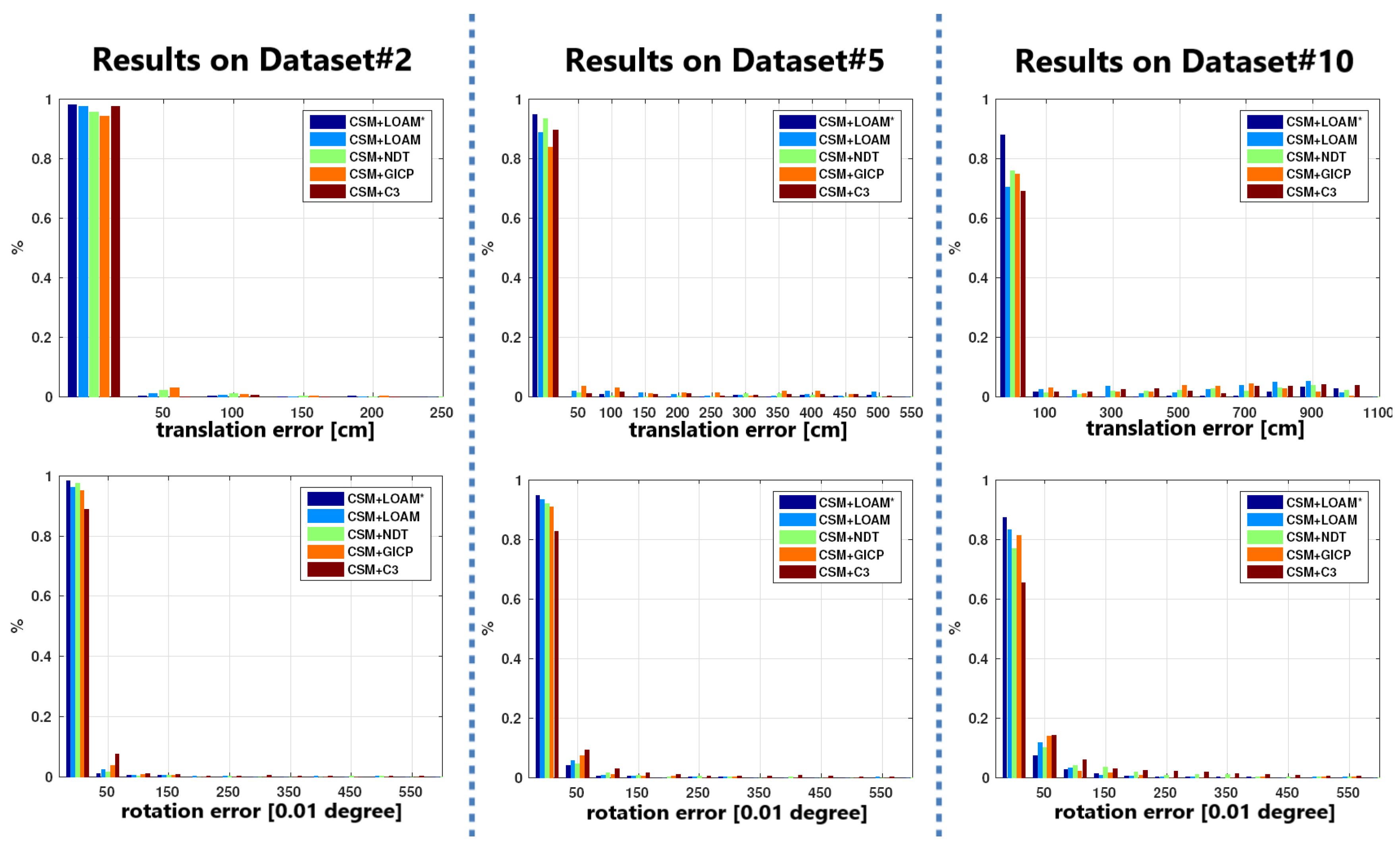
The proposed method is tested on Dataset#2, Dataset#5 and Dataset#10. The proposed method is called CSM+LOAM∗, in comparison to CSM+LOAM which has no sampling step and only pass one transformation is passed from CSM to LOAM. CSM is also combined with GICP and NDT. The results are shown in Figure 7.

As can be seen from Figure 7, the proposed method performs best on all datasets. Since CSM+LOAM∗ is more accurate than CSM+LOAM, it proves that the proposed sampling and evaluation mechanism is effective.

Comparing Figure 3 and Figure 4 with Figure 7, it can be noticed that the performance of the combined method, including CSM+GICP and CSM+NDT, is much better than the original GICP or NDT, especially in Dataset#5 and Dataset#10. This shows that the proposed sampling and evaluation techniques can be generally adopted to improve the performance of any local scan matching method.

5.4. Computational Complexity Analysis

The proposed ‘CSM+∗’ (where ‘∗’ represents any local scan registration approaches) approach mainly consists of two parts: the CSM part and the local scan registration part. Other than that, the computation of the sampling and the evaluation part is neglectable. Let $t_0$ and $t_1$ represent the computation time of the CSM algorithm and the local scan registration algorithm respectively. n represents the number of sampled transformations passed from CSM to local scan registration approach. Therefore, the overall computational time of the proposed ‘CSM+∗’ will be $t_0+n\ast t_1$. It could be further accelerated to $t_0+t_1$ if the n local scan matchers run in parallel.

6. Conclusions

This paper studies the problem of scan registration in an off-road environment. Several scan registration approaches, both local and global methods, were evaluated on a newly created dataset. Experimental results indicate that, whilst local scan registration approaches, i.e., LOAM, performs best on small offset dataset, a global scan registration approach, i.e., CSM, performs better on large offset dataset. To combine the advantages of both approaches, a sampling and an evaluation algorithm is proposed. Further experiments show that the sampling and evaluation techniques can improve the performance of any local scan registration approaches, thus making it a universal method.

References

- Castaño, F.; Beruvides, G.; Villalonga, A.; Haber, R.E. Self-tuning method for increased obstacle detection reliability based on internet of things LiDAR sensor models. Sensors 2018, 18, 1508. [Google Scholar] [CrossRef] [PubMed]
- Castaño, F.; Strzełczak, S.; Villalonga, A.; Haber, R.E.; Kossakowska, J. Sensor reliability in cyber-physical systems using internet-of-things data: A review and case study. Remote Sens. 2019, 11, 2252. [Google Scholar] [CrossRef]
- Arun, K.; Huang, T.S.; Blostein, S.D. Least-Squares Fitting of Two 3-D Point Sets. IEEE Trans. Pattern Anal. Mach. Intell. 1987, 5, 698–700. [Google Scholar] [CrossRef] [PubMed]
- Segal, A.V.; Haehnel, D.; Thrun, S. Generalized-ICP. In Proceedings of the Robotics: Science and Systems, Seattle, WA, USA, 28 June–1 July 2009. [Google Scholar]
- Biber, P.; Straßer, W. The normal distributions transform: A new approach to laser scan matching. In Proceedings of the International Conference on Intelligent Robots and Systems, Las Vegas, NV, USA, 27–31 October 2003; pp. 2743–2748. [Google Scholar]
- Magnusson, M. The Three-Dimensional Normal-Distributions Transform: An Efficient Representation for Registration, Surface Analysis, and Loop Detection. Ph.D. Thesis, Orebro Universitet, Örebro, Sweden, 2009. [Google Scholar]
- Zhang, J.; Singh, S. LOAM: Lidar Odometry and Mapping in Real-time. In Proceedings of the Robotics: Science and Systems, Berkeley, CA, USA, 12–16 July 2014; pp. 1–8. [Google Scholar]
- Olson, E. Real-Time Correlative Scan Matching. In Proceedings of the IEEE International Conference on Robotics and Automation, Kobe, Japan, 12–17 May 2009; pp. 4387–4393. [Google Scholar]
- Chen, Y.; Medioni, G. Object modeling by registration of multiple range images. In Proceedings of the IEEE International Conference on Robotics and Automation, Sacramento, CA, USA, 9–11 April 1991; Volume 3, pp. 2724–2729. [Google Scholar] [CrossRef]
- Stoyanov, T.; Magnusson, M.; Andreasson, H.; Lilienthal, A.J. Fast and accurate scan registration through minimization of the distance between compact 3D NDT representations. Int. J. Robot. Res. 2012, 31, 1377–1393. [Google Scholar] [CrossRef]
- Shan, T.; Englot, B. LeGO-LOAM: Lightweight and Ground-Optimized Lidar Odometry and Mapping on Variable Terrain. In Proceedings of the IEEE International Conference on Intelligent Robots and Systems, Madrid, Spain, 1–5 October 2018; pp. 4758–4765. [Google Scholar] [CrossRef]
- Sun, B.; Kong, W.; Xiao, J.; Zhang, J. A hough transform based scan registration strategy for Mobile Robotic Mapping. In Proceedings of the IEEE International Conference on Robotics and Automation, Hong Kong, China, 31 May–5 June 2014; pp. 4612–4619. [Google Scholar] [CrossRef]
- Levinson, J.; Thrun, S. Robust vehicle localization in urban environments using probabilistic maps. In Proceedings of the IEEE International Conference on Robotics and Automation, Anchorage, AK, USA, 3–7 May 2010; pp. 4372–4378. [Google Scholar]
- Wolcott, R.W.; Eustice, R.M. Fast LIDAR Localization using Multiresolution Gaussian Mixture Maps. In Proceedings of the 2015 IEEE International Conference on Robotics and Automation (ICRA), Seattle, WA, USA, 26–30 May 2015; pp. 2814–2821. [Google Scholar]
- Fu, H.; Yu, R.; Ye, L.; Wu, T.; Xu, X. An Efficient Scan-to-Map Matching Approach Based on Multi-channel Lidar. J. Intell. Robot. Syst. Theory Appl. 2018, 91, 501–513. [Google Scholar] [CrossRef]
- Chong, Z.J.; Qin, B.; Bandyopadhyay, T.; Ang, M.H.; Frazzoli, E.; Rus, D. Mapping with synthetic 2D LIDAR in 3D urban environment. In Proceedings of the IEEE International Conference on Intelligent Robots and Systems, Tokyo, Japan, 3–7 November 2013; pp. 4715–4720. [Google Scholar] [CrossRef]
- Kanade, B.D.L.; Takeo. An Iterative Image Registration Technique with an Application to Stereo Vision. In Proceedings of the International Joint Conference on Artificial Intelligence, Vancouver, BC, Canada, 24–28 August 1981; pp. 674–679. [Google Scholar]
- Grisetti, G.; Kummerle, R.; Stachniss, C.; Burgard, W. A tutorial on graph-based SLAM. IEEE Intell. Transp. Syst. Mag. 2010, 2, 31–43. [Google Scholar] [CrossRef]
- Dellaert, F.; Kaess, M. Factor Graphs for Robot Perception. Found. Trends Robot. 2017, 6, 1–139. [Google Scholar] [CrossRef]
- Gao, Y.; Liu, S.; Atia, M.M.; Noureldin, A. INS/GPS/LiDAR integrated navigation system for urban and indoor environments using hybrid scan matching algorithm. Sensors 2015, 15, 23286–23302. [Google Scholar] [CrossRef] [PubMed]
- Kaess, M.; Member, S.; Ranganathan, A. iSAM: Incremental Smoothing and Mapping. IEEE Trans. Robot. 2008, 24, 1365–1378. [Google Scholar] [CrossRef]
- Fu, H.; Zhang, Q.; Qiu, G. Random Forest for Image Annotation. In Proceedings of the European Conference on Computer Vision (ECCV), Florence, Italy, 7–13 October 2012; Volume 7577 LNCS, pp. 86–99. [Google Scholar] [CrossRef]
© 2020 by the authors. Licensee MDPI, Basel, Switzerland. This article is an open access article distributed under the terms and conditions of the Creative Commons Attribution (CC BY) license (http://creativecommons.org/licenses/by/4.0/).