Development of a Practical Tool for Designing Multi-Robot Systems in Pick-and-Place Applications

Abstract

Pick-and-place manipulators have become one of the principal components of almost all manufacturing plants. The process of sizing the number of manipulators required to efficiently carry out pick-and-place tasks depends on the complexities of such plants, the characteristics of the production line and the particular requirements. These aspects tend to make the sizing procedure rather complex and time consuming. Moreover, the results are closely linked to the accuracy of the input data that is usually, especially in the initial stages, unreliable and haphazard. To face these issues, the simulation tools currently available in the market are not always suitable. In this paper, a practical procedure to size the number of manipulators required in any particular plant to perform pick-and-place tasks is presented. This procedure results in a relatively simple tool capable of calculating the number of robots required in a line knowing the layout, type of robot to be used, and production characteristics. This tool is able to simulate the different distribution of goods on the line as well as the required strategies for picking in a multi-robot environment to test several production situations and assess the accuracy of the sizing.

1. Introduction

Pick-and-place robots are essential in industrial systems due to their effect on saving labor costs [1], and doing required tasks rapidly and accurately [2,3]. In particular, they can be used to perform different tasks depending on the production requirements. Mainly they are used for assembling, packaging, bin picking, inspecting, and picking and placing products from one conveyor belt to another [4,5]. Although the use of pick-and-place systems in industrial applications has been operative for many years, the design process must deal with many challenges which have yet to be overcome. The sizing process of a team of robots to be used in pick-and-place applications is a lengthy and usually complicated process since it depends on an high number of variables that are sometimes unknown, or not easily measurable and, when measured, may assume different or random values during execution. For these reasons, the design process of the multi-robot system becomes complex and usually heuristic methods are used to perform this task [6].

To address the problem statement, the sizing procedure must take into consideration a large number of variables which can be grouped into four main categories:

• Product characteristics: depending on the production in terms of the number of products that have to be picked in a given time together with the consideration of how these products are distributed on the conveyor belt, i.e., in a constant flow or haphazardly. The size of the product as well as the distance between them also affects the result.
• Robot characteristics: the robot type [2,7] affects the cycle time or time required to do a pick-and-place task. Characteristics such as the type of gripper influence how many parts are picked at the same time. The motion control law [8] used to define the dynamics and the trajectory planning optimization algorithm [9] to pick and to place different parts has also to be taken into consideration.
• Item assignment algorithm: When more than one robot is used for pick-and-place applications one must use an optimal control logic to coordinate the set of robots to have optimum performance [10]. It is important to use efficient task assignment algorithms to divide in a cooperative manner [11] the items over the conveyor among the team of robots. Picking the maximum number of items within the least time without losing parts is subsequently translated into fewer robots and thus less cost [12,13]. These algorithms can be divided into two different categories, in the first an overall cost function is calculated and minimized for every product to be picked to decide the group of the product to be assigned for every robot. In the second each robot calculates and minimizes on its own a cost function based on the products it has detected within its workspace (the set of all positions that a robot can reach) in order to define the items to be picked.
• Scheduling algorithm: This regards the definition of the order in which every robot should pick and place the items assigned [14] taking into account the distance between the robot and the items as well as the cycle time. To confront this issue, scheduling algorithms such as “First in first out” (FIFO), “Last in first out” (LIFO), “Shortest process time” (SPT), “Second shortest product time” (SSPT) [15] and the like can be used. To be able to compare different scheduling rules, the picking rate is used as the comparison parameter and this is given by the ratio between the objects picked using a given rule and the total number of objects.

Taking into account the above-mentioned variables, one can describe most of the situations in which products have to be picked and placed using a multi-robot system. In the industrial or in academic world there are no consolidated standard mathematical formulae or systematic ways that can be used to determine the number of robots necessary to be used for these applications. Mainly, heuristic methods are used, depending on the experience of the operator in charge of the sizing task.

Moreover, the available software on the market capable of simulating a multi-robot environment and collaborative algorithms to control them and production flow requires a complete description of the system and a knowledge of all the physical parameters previously described. Robotic system simulators such as V-rep [16] or Gazebo [17] allow one to describe in detail complex production lines in which multi-vendor robots cooperate to produce items or software simulator such as Mitsubishi RT-toolbox, ABB Robot studio and the like can assist in designing robotic cells and in programming the behavior of the robots. The above-mentioned simulators are able to describe all the aspects of a production line but they require a long time to develop simulations, high programming skills and a full knowledge of production parameters and are therefore not suitable for the initial phase of the sizing task of a multi-robot line. In this phase, usually called budgeting or pre-sizing, there are too many unknown factors, and to work with this software is useless.

In this paper, a simplified and practical approach to assist the process of sizing multi-robot scenarios is proposed. The idea based on this work is to develop a tool that is easy to use and simple to be configured with the parameters available in the early stage of the design of a production line. The output of the above-mentioned tool is the number of robots required to serve a line given a general description of the plant, the type of used robots, the task assignment algorithm, and summarized production data.

2. Industrial Empirical Sizing Procedure

The common approach to size a multi-robot scenario uses the following formula [6]:

$$N{R}_{min}={\displaystyle \frac{FPs\ast (1+Mfp)}{PPas}}$$

(1)

where $N{R}_{min}$ is the minimum number of robots required, $FPs$ is the input product per second and $MfP$ is the product flow safety margin. Whereas $PPas$ is the product cadence (picked and placed products per second) defined by:

$$PPas={\displaystyle \frac{1}{t_{pick}+t_{place}+t_{translation}}}$$

(2)

The above formula is dependent on the following assumptions. The “input product flow rate” is known and chosen on basis of production requirements usually expressed as the average value of the number of products per second. The “product cadence per second” indicates the number of products that can be picked by a robot per second. This number can be evaluated from the robot data sheet which is equal to the inverse of the task execution time. Product cadence depends on three main elements: picking time ($t_{pick}$), placing time ($t_{place}$) and the time required to move from the picking point to the placing one ($t_{translation}$). The latter depends on the technical characteristic of the robot, such as speed, acceleration, and the distance to be covered by the end effector of the robot to reach the products.

Please note that this formula is based on an ideal production situation. Thus, it does not take into account the common variables within a production line such as: variable input product flow rate, varying distance between products, variable position of the product along the conveyor belt, different strategies of pick-and-place in a multi-robot situation (i.e., the algorithm used to coordinate several robots working together) and individual scheduling algorithms which optimize the pick-and-place tasks. Therefore, the sizing procedure based on the formula [6] is only a guideline and far from being a reliable method of calculating the number of robots required in a given production line. This is particularly true in the case where the above factors are pre-eminent. To overcome these issues and provide to the designers a useful design tool, a sizing procedure based on a practical approach is presented in this paper.

In particular the proposed procedure is aimed at designers that need to rapidly calculate the number of robots required to set up a production line. During the initial development phases of a production line or during the calculation of the costs related thereto, it is often impossible to know all the details required to work out exactly how many robots are necessary. It is however fundamental to be able to evaluate either effects of the variation in production or those of the collaboration strategies between the robots on the number of pieces to be picked by the manipulating system. In this way one can size the production line with greater reliability and it is easier to attain the required performance.

Modern literature focuses mainly on the optimization of performance of a given pick-and-place robotic system. For instance, this is obtained through the optimization of the pick-and-place operation to improve the efficiency of assembly tasks [18], or minimizing the distance to be travelled by the robot arm through the use of genetic algorithms as presented in the paper [19]. In other contexts, the minimization of the cycle time passes through the optimization of the feeder assignment and the pick-and-place sequencing [20]. In all these cases the production line has already been realized and the approaches used to analyze end improve the performance of the system are not suitable for the sizing purposes.

The problem of the multi-robot system sizing for pick-and-place applications is not extensively analyzed in the literature especially in the early stages of the development of a production line. To the knowledge of the authors the Equation (1) represents the state of art for industrial applications. This paper suggests an alternative approach which is easily applicable and suitable for early design stages. In particular, this paper proposes a practical approach based on the simplification of the robot movement during picking and placing tasks but substantially maintaining the same cycle time. Moreover, this method allows one to take into account the collaborative strategies between robots and spatial and temporal variability of the products distributed along the production line. In the following section this method is described in depth.

3. Practical Sizing Tool

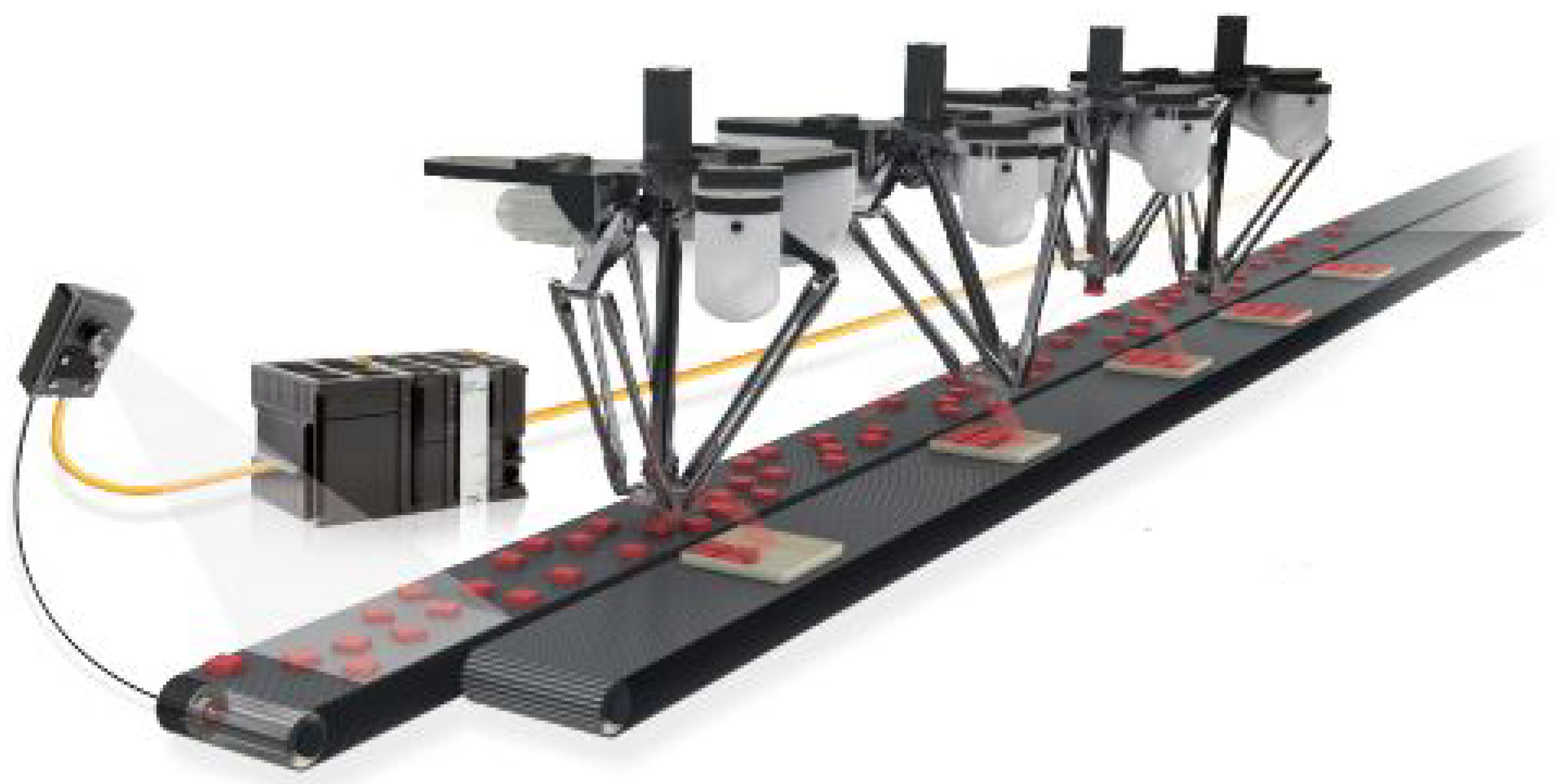
The practical sizing tool has been developed with MATLAB environment and allows one to size the number of robots required to serve a production line where products are moving along a conveyor belt and picked by robots as shown in the Figure 1.

Using this tool, the designer takes into consideration different operating conditions and collaboration strategies between robots. In particular, one can easily change the input parameters to describe different operating conditions such as variation in production flow rate (for instance random or constant), or “picking and placing” positions (in the area in which a robot can pick an item) and generic dimensions of the line layout and the like. Multi-robot pick-and-place systems are used in many production lines, so different products with different characteristics are usually handled and must be taken into consideration. Since the purpose of this work is to create a flexible universal sizing tool that can be used for the maximum possible number of different applications without the need to change the core of the tool, some assumptions about the production line are done to overcome problems related to the diversity of products, layout, robot characteristics, and the like.

The following subsections describe the main elements of a production line that must be standardized and represented to obtain a flexible sizing tool. These are substantially four: plant, production, strategies, and robot representation. These elements are presented and commented on in detail hereafter, moreover the way in which they are included and taken into consideration within the sizing tool is described.

3.1. Production Plant Description

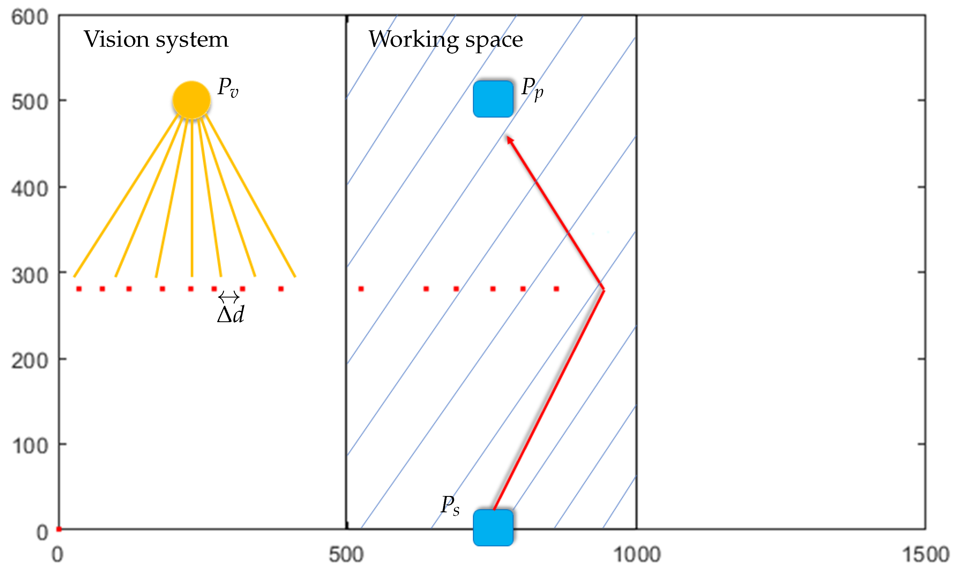
A generic production plant, served by a multi-robot pick-and-place system, is described, in the sizing tool, through the representation of the areas in which each robot can pick an item on the conveyor belt. These areas are called robot working area and described by a rectangle. The hatched area in Figure 2 represents the working area of a generic robot operating on a conveyor belt. In this area two points are shown: the starting point ($P_s$) of the end effector of the robot (the device at the end of a robotic arm) and the placing point ($P_p$). Respectively they are the position where the end effector begins its movement and the position where the picked item must be placed.

The items are moving along the conveyor belt as indicated by the arrow in Figure 2. The position of the objects to be picked is detected by a vision sensor [21] that is usually placed in front of the robot working spaces. The vision sensor or the camera continuously photographs the conveyor belt to detect the positions of the objects. The vision sensor position ($P_v$) and in particular the distance between the camera and the working area of the robot, is an important parameter that has to be taken into consideration in order to guarantee optimum performance of the system and effects the final result of the sizing procedure. The vision system detects the objects on the conveyor belt as soon they enter into its vision radius and determines the coordinates of the center or the picking point of each object [22].

In the sizing tool the items are represented through the coordinates of points that moves along a linear trajectory with constant speed. The coordinates of each item represent the positions of the product immediately before they enter within the working area of the robot. Since the distance between products and the position of the working area of the robot is known, considering the speed of the conveyor belt (input parameter of the sizing tool) one can accurately simulate the product behavior along the production line. The layout of the production plant is described by a set of coordinates (

Table 1. Parameters used to describe the plant.

Parameter	Description
$P_p$	Placing position
$P_s$	Starting position
$P_v$	Vision sensor position
$\Delta d$	Distance between products (random, constant)
$\Delta y$	Range of space in which the products are placed

) that defines the position of the vision system, the starting and placing points of the end effector within the working area and the dimensions of the latter for each robot.

3.2. Production Description

In actual applications, the most important parameter that describes the production is the product flow rate which gives an idea of how many objects will be placed on the belt per time unit. Starting from this parameter it is possible to generate products that simulate different production situations.

For instance, when the product flow rate is constant, the distance between an item and the following one is usually the same and all of them are distributed along the axis of the belt. This is the ideal situation for a production system. This behavior can be found in applications that require high accuracy such as for electronic chip production systems where the belt is moving slowly and the position in which the product has to be picked is calculated precisely. On the contrary, in some food industries such as fresh fruit and vegetables, the situation is different. The production line has a certain average product flow rate but variable in the period, the product distribution results in a different distance between each item along the conveyor belt.

During the designing phase, one has to consider furthermore, the situation in which the products to be picked are randomly distributed in both of the dimensions of the conveyor belt, this represents the most complicated situation that can happen and the pick-and-place system has to deal with. The complexity is due to the fact that the distance that the robot end effector has to follow during the pick-and-place task for different products is continuously changing and it may happen that few consecutive objects are at the maximum distance from the robot position so the cycle time to execute those tasks is lengthy and would thus significantly increase the probability of losing some of those products. The number of lost products is a very important parameter to describe the efficiency of the system, so it must be the minimum possible value.

To generate the product distribution the tool developed uses the function of MATLAB called rand (function that generates arrays of random numbers whose elements are uniformly distributed), taking into account the minimum distance between two consecutive objects depending on the product length and the average product flow rate. It is also important to define a maximum range within which the objects are distributed, and the working space that will affect the maximum distance travelled, and thus the cycle time.

With the above-mentioned method, one can consider the behavior of different production systems which is important during the design procedure because it permits the testing of the stability of the system against random pattern variation.

3.3. Task Assignment Algorithms

The tool is used basically to help the designer during the design process to simulate different conditions and evaluate the response of the system before installation. Therefore different task assignment algorithms are required to distribute products to several robots, because according to the algorithm used, different results can be obtained such as the percentage of the product picked by every robot, the workload or the period of time in which the robot is working, and the waiting time.

Those parameters are important to be evaluated because they give an idea about the consumption of the robot and this is extremely valuable since it gives an estimation of the working life of the robots (the complete amount of time for which a robot can be expected to operate) and useful also to schedule the regular maintenance for every robot of the system.

Using the developed tool one can choose from three different assignment algorithms well known in scientific literature [6]:

• First in first out (FIFO). It is the simplest rule because it does not require any calculation to determine which item has to be picked first. The first item detected that enters the working space of the robot is the one to be picked. This rule has a disadvantage since the first robots in the pick-and-place system work more than the rest of the team, which may in fact shorten the working life of these robots. To implement this rule, consider a system similar to Figure 2. When objects enter the working space, these are assigned to the first robot that picks them in the same order in which they entered the working space. The objects missed by the first robot are assigned to the second one in the same order they enter its working space.
• Up to down. This rule consists of a distribution of items to be chosen by the robots based on the distance between them and the placing positions. These distances are calculated when the items are detected by the vision system. After putting the distances in ascending order, on can assign items to the robots so that the nearest item is assigned to the first robot and the farthest one is assigned to the last robot. Generally, this rule requires one to make numerous calculations to assign items to the robots compared to the FIFO rule. It has the advantage of being more efficient for fast pick-and-place applications since the first robot picks up a greater number of items (the ones nearest to the robot), in a short time. Figure 2 shows a typical layout required by this assignment rule. Cyclically, the distances between the items placed on the conveyor belt and the placing positions are calculated. The item with the minimum distance between itself and the placing position, in the upper part of the conveyor belt shown in the figure, is assigned to the first robot. The item with greater distance is assigned to the second robot and so on until assigning the item with the greater distance to the last robot.
• Right to left. The working principle is analogous to the previous rule. A vision system detects the object on the belt, and they are being distributed to the robots based on the time in which they enter the working space. It is assumed that the items are generated on the left side of the belt as shown in Figure 2. Thus, in the photo of the detected objects, the items on the right side will be the first to enter the robots working space. To implement this rule, the objects are assigned to the different robots as soon as they enter the working space of the multi-robot system. The first object is assigned to the first robot and the following one is assigned to the second robot until the assignment of objects to all members of the team of robots. This operation is repeated continuously.

3.4. Robot Behavior Description

The dynamic behavior of the robot to be used in a pick-and-place task is difficult to simulate because it depends not only on the specific kind of robot to be used but also on the specific scenario. This depends largely on the physical design of the robot, its number of degrees of freedom, the length of the linkages and the characteristics of the motors such as angular speed, acceleration, torque, and the like. Moreover, in industrial applications the object is picked by the robot after a tracking path. Through this trajectory planning procedure, the robot reaches the current position of the product and follows it for a certain distance to ensure that in the picking position the end effector will have the same speed and position of the product. The tracking process differs greatly between different robot manufacturers. Moreover, the techniques used are in continuous development to affects the efficiency of the pick-and-place systems.

To simplify the robot behavior description, this is substituted by the movement of the end effector in a two-dimensional working space. The trajectory of the end effector is described with lines followed with a constant speed properly determined. This speed is the one that allows the end effector of the robot to perform a pick-and-place task with the same time as the actual robot does. As explained above, the coordinates of the placing and picking position, having been calculated, are subsequently transmitted to the robot moving towards the item. Thus, the position of each product is the only information required by the sizing tool developed.

3.4.1. Picking Position Calculation

When an item enters in the working space of a robot, such robot determines the nearest picking position based on the data available. If the picking position is outside of the robot working space, the latter moves on to the following product and the item not picked up is considered lost. Therefore, to generalize the problem, one can simplify the trajectory followed by the end effector of the robot taking into consideration the nearest possible picking point reachable by the robot. To determine such point, one should know the values of the following parameters:

• $x_r,y_r$ Robot current position
• $V_r$ Robot average speed
• $x_p,y_p$ Product current position
• $V_p$ Product speed (conveyor speed)

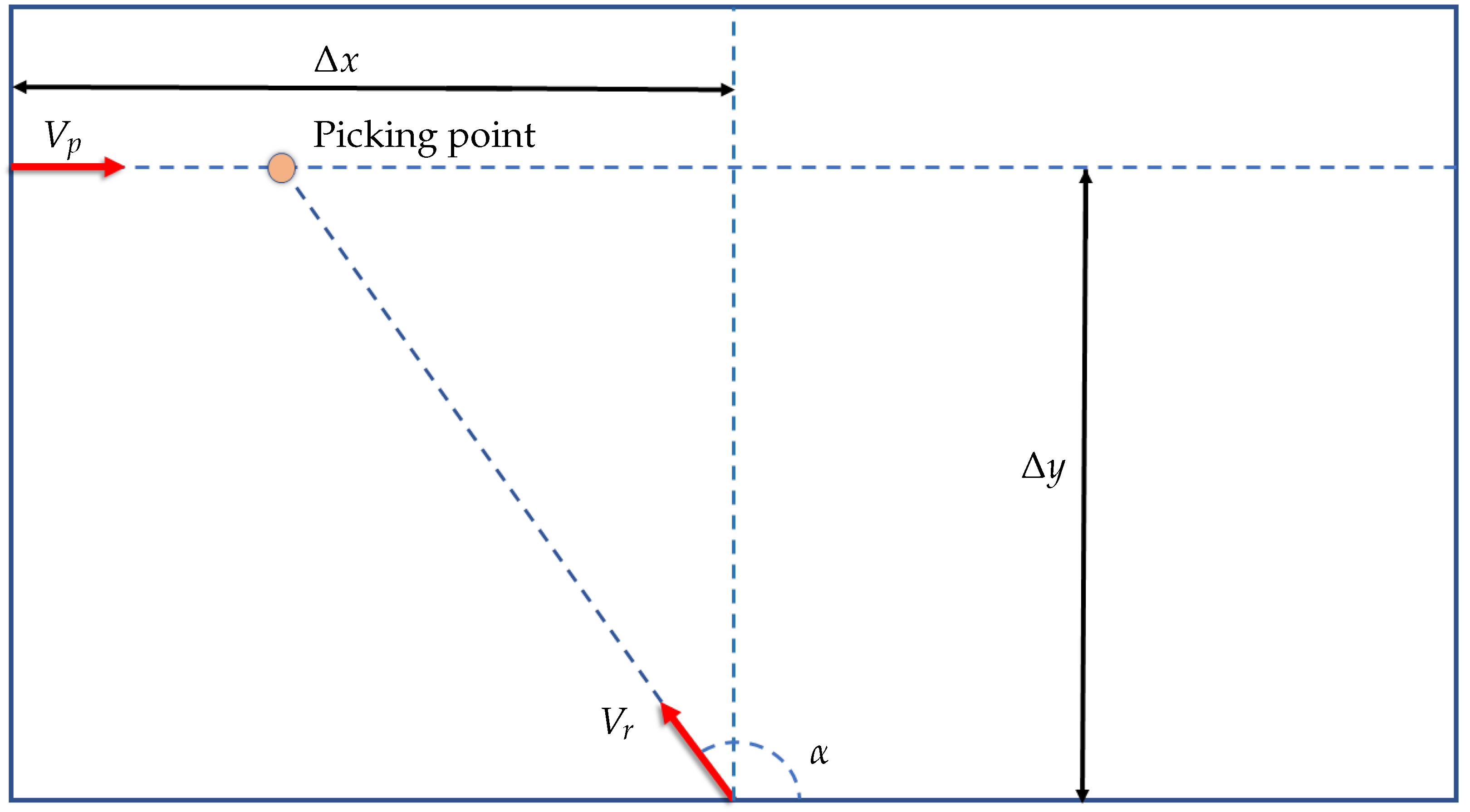
Knowing those parameters one can determine the picking position solving the following equation system:

$$\left\{\begin{array}{c}{V}_p·t_p=x_p\hfill \\ x_p=\Delta x+V_r·cos\left(\alpha \right)·t_p\hfill \\ V_r·sin\left(\alpha \right)t_p=\Delta y\hfill \end{array}\right.$$

(3)

where $t_p$ is the time required for the robot to reach the product, $x_p$ is the picking position, $\alpha$ is the angle between the abscissa and the linear trajectory followed by the end effector, as shown in the Figure 3.

In actual applications, the behavior of pick-and-place robot may differ slightly from the one described. In fact, in order to decrease the cycle time for pick-and-place tasks, the end effector of the robot is placed in a particular position, called the waiting position, close to the picking point before the product enters in the working space. Figure 4 shows and example of the wait and pick position on a conveyor belt. The robot moves into the waiting position at the start of its work cycle. When the product enters in its working space, the robot moves to meet the product on the picking position calculated. Please note that the distance covered by the robot is less than the one covered when the robot is waiting for the following product in the placing position. The waiting position is an important parameter that can be easily defined in the sizing tool developed as well as the placing position. Whereas the picking point is calculated by following the above-mentioned strategy where the end effector is moved along the trajectory with a constant average speed.

Thus, the dynamic behavior of the robot is simplified and the most important parameter to be determined, in order to obtain reliable results, is the average speed which the end effector must have in order to complete the cycle time as the robot would have had with a variable speed profile.

3.4.2. Robot Speed Characterization

The robot speed characterization is the crucial point of this procedure. Obviously, the value of the average speed required in the sizing tool is not given by the manufacturer of the robot. The latter can only give speed values related to specific tasks such as the maximum end effector speed when it moves following a horizontal direction or speed profile and cycle time required to perform pick-and-place tasks in continuous mode considering an arbitrary distance. This information does not allow one to calculate the average speed. This depends on application parameters such as the picking, placing, and waiting positions and the like.

To develop a simple software tool that works for different robots, the following steps should be taken. Having to size a production line with multiple robotized picking and placing stations one has to take into consideration a generic workstation and perform some tests in order to determine the average speed. A single pick-and-place manipulator is used and its behavior is simulated while executing few pick-and-place tasks. These simulations are relatively simple to do by the use of professional robotic simulators that are provided by the robot manufacturers and that assist in programming and developing application for their robots.

The purpose of these simulations is to reproduce exactly the behavior of the relevant robot with the least number of approximations. Using these tools in fact the tracking trajectory is reliably reproduced together with the dynamics of the robot. These are all aspects that directly affect the cycle time of each pick-and-place task. Developing a single pick-and-place station with this software is relatively simple and does not require robot coordination strategies, precise working scenario definitions, and the like. After execution, the simulation of this simplified scenario, some important information is collected such as the cycle time, waiting time, and distances covered by the robot.

The same operating scenario is simulated by using the design tool developed, configured to the parameters above-mentioned and collected in order to determine the value of average speed that allows one to obtain the same approximate cycle time during the pick-and-place operation.

3.5. Number of Robots and Performance Evaluation

To determine the number of pick-and-place stations required to size a production line, one must use some performance indexes. The sizing tool developed repeats the simulation of picking and placing tasks of the products according to the set-out modalities and with the input parameters furnished by the designer by progressively adding robotic stations until reaching the required performance value indexes.

Through these, the tool can determine the number of robots to be used to guarantee the required operating function of the production line. The performance indexes used are obtained from scientific literature [6,15] and industrial applications and can be mixed between them according to the circumstances. The most important of these are itemized below.

• Picking rate: define the ratio between the sum of the products picked by all the robots and the number of products available on the conveyor.

  $$M_i=\frac{{\displaystyle \sum _{j=1}^n}{N}_j}{N}$$

  (4)

  where $i=1,......,m$, indicates the used coordination algorithm among m possible algorithms, $j=1,......,n$, n is the number of robots used, $N_j$ is the number of picked products by the robot j using the i coordination algorithm and N is the number of products to be picked.
• Workload of every robot: identify the ratio between the time period in which the robot is computing the pick-and-place task and the overall time including the waiting time.

  $$W=\frac{t_{picking}+t_{placing}}{t_{picking}+t_{placing}+t_{waiting}}$$

  (5)

  where W is the Workload, $t_{picking}$ and $t_{placing}$ are the time necessary to execute the task, whereas $t_{waiting}$ is the waiting time between two pick-and-place tasks in which the robot is available but with no-product to be picked.
• Balance of the workloads: it is given by the comparison between the individual workloads of the team.

  $$B=\sum _{j=1}^{n-1}\left|W_j-W_{j-1}\right|$$

  (6)

  where B is the balance value, $j=1,....,n$, n is the number of used robot and $W_j$ is workload of the robot number j. The balance value is defined as the difference of the workload of the robots. The system is more balanced when the balance value is close to zero.
• Total workload: gives an idea of how much the system is used and it is given by the sum of all the workloads of all the robots.

  $$TW=\sum _{j=1}^n{W}_j$$

  (7)

  where $TW$ is the total workload and $W_j$ is the workload of the $j_{th}$ robot.

4. Test Case and Results

In this section, an actual industrial project is considered, and the developed tool is used to determine the number of robots for a pick-and-place application based on a multi-robot system. The following describes the problem to be solved. This problem can be considered a typical issue to be resolved in the quotation phase for the number of robots necessary to pick the products from the conveyor belt.

4.1. Actual Project

In this particular case, a pick-and-place system must pick syringes from one conveyor belt and place them on another one in groups which thereafter must be packed. The problem is to calculate the number of robots required in order to guarantee a product flow rate of 160 products per second. Other information usually supplied for the sizing of the robot line is set out below:

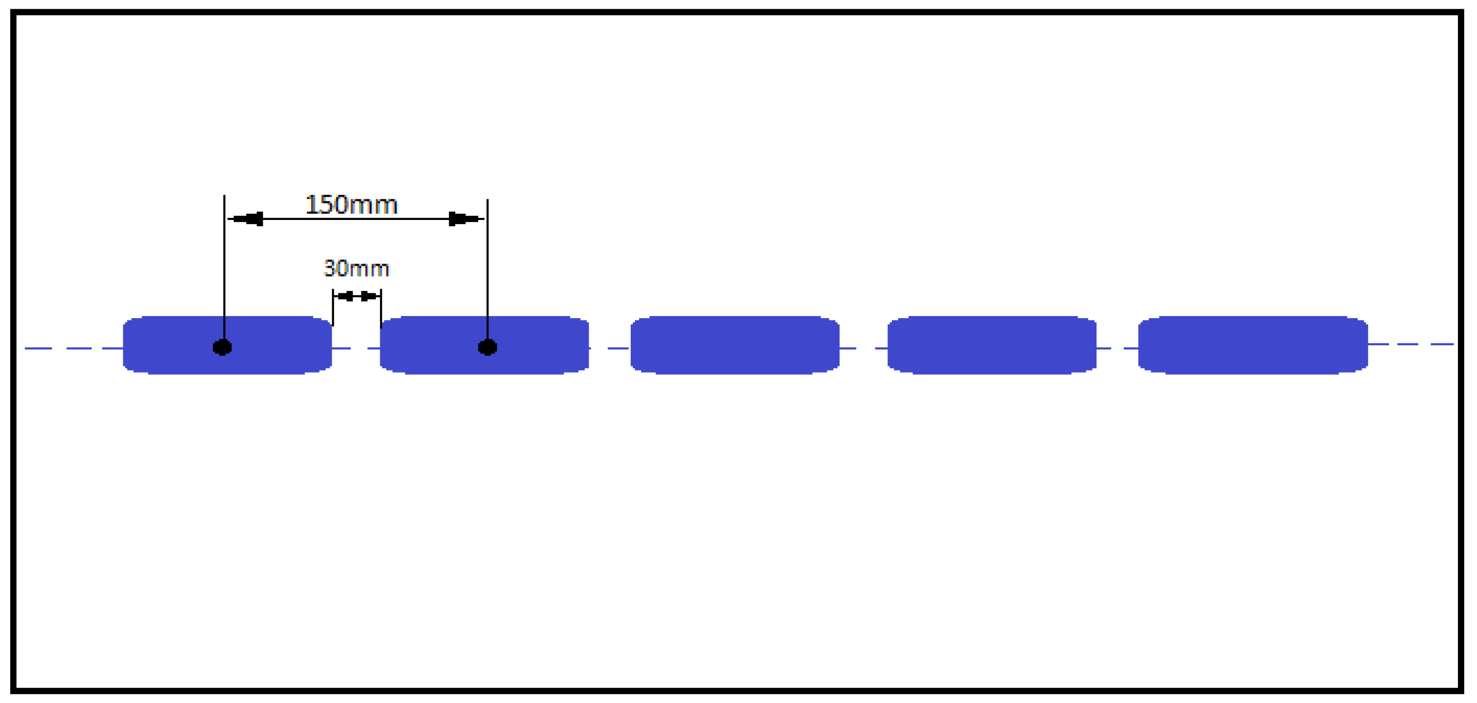
• Product dimensions: 120 × 20 mm (Syringe in nylon bag)
• Products displaced longitudinally with distance about 30 mm between them
• Production flow rate: 160 product/second
• Conveyor speed: 24 m/s
• Conveyor width: 100 mm
• Maximum distance between picking position and placing position: 240 mm
• Placing with rotation of 90 degrees
• Step of output conveyor to filling machine for syringe: 127 mm(max speed 20.3 m/s)

Other information relates to the robotic solution to be used. Specifically, in the example under consideration we will use a task assignment logic for the distribution of the work in which the first robot picks the first product the second robot the second one and so on. Moreover, regarding the plant layout, we will use the Mitsubishi SCARA robot RH1FHR5515 series and we will work with a placing time of 100 ms and picking time of 50 ms. Figure 5 shows how the products will be distributed on the production line.

The above information is sufficient to calculate the number of robots required using Formula (1), and this case the result is 1.2 robots. This means that 2 robots are required to pick all the items on the line without losing any. In effect, the parameters provided for sizing are nominal values and do not take into consideration phenomena such as products missing along the line, distance variation in the products, and the like. The tool developed is also capable of taking into consideration such phenomena to allow one to obtain a more accurate sizing. Moreover, in the preliminary stage, one can also evaluate the effects of the distance between the robots in the performance of the entire systems.

4.2. Average Speed Determination

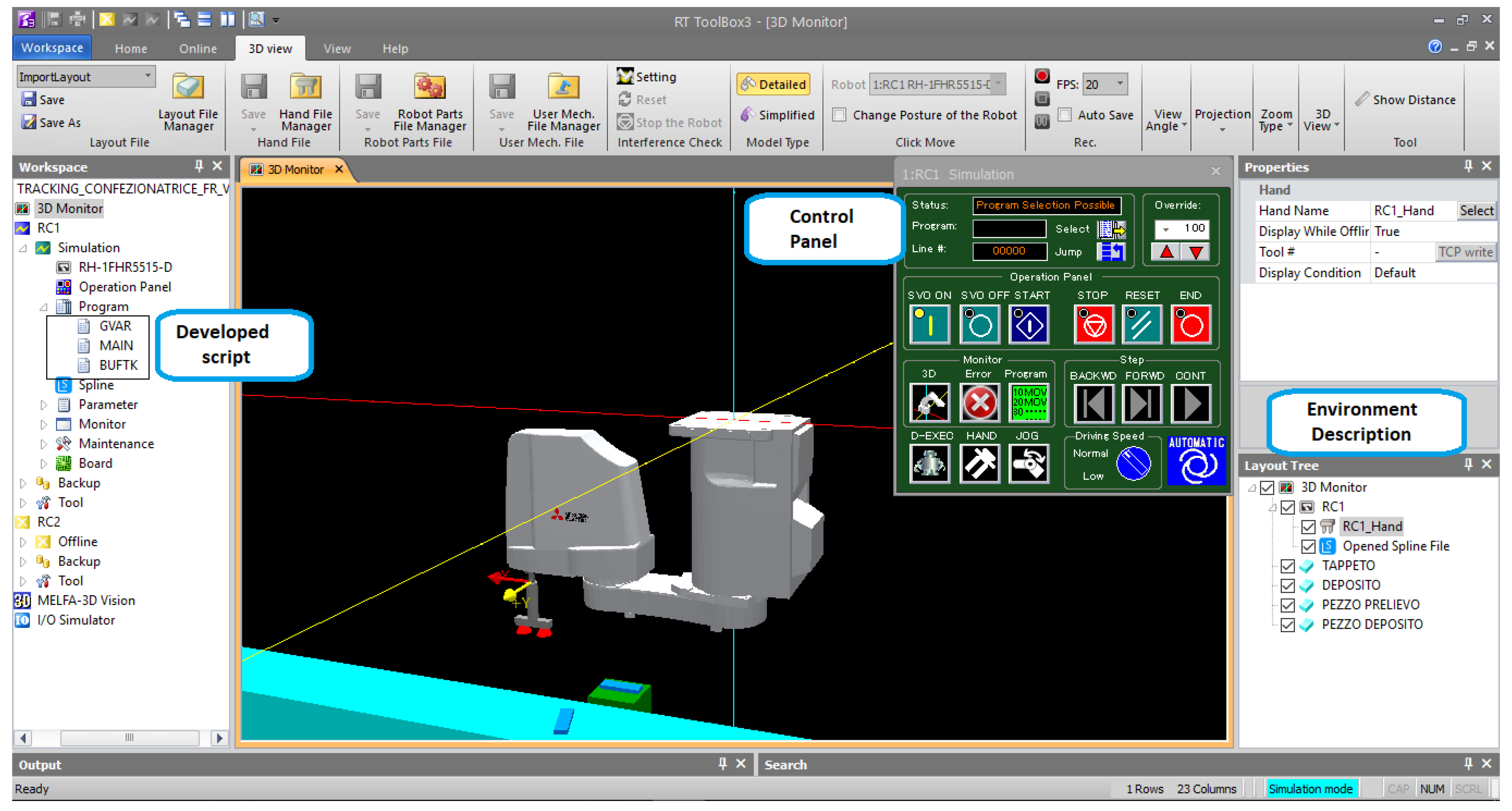
The fundamental parameter required to use the sizing tool is to determine the average speed of the robot that one has chosen to use in the application. Therefore, a simulation needs to be carried out especially taking into consideration the robot model to be installed. The test consists of the use of the manufacturer robotic simulator environment (in this case being the Mitsubishi RT-toolbox) to simulate the behavior of a single robot station while executing pick-and-place tasks. Such simulation allows one to define the value of the average speed for the sizing procedure.

Please note that the use of such simulators requires a thorough knowledge of robotics and of robot programming language. Such simulators are in fact used by developers for programming and functioning the production lines. Thus, the time required to effect the simulation is identical to that needed to develop the final system project and needs to take into consideration the task assignment logic to the robots, the sensors present in the line, the presence of possible obstacles, etc. Thus, the simulation of the entire system is impossible in the preliminary sizing phases required for the pricing of the line because it is not economically viable and one therefore uses the Formula (1).

The simulation and programming of a generic picking station with the development environment produced by the robot manufacturers can be taken and used to determine the average speed required by the sizing tool without wasting too much time. Moreover, having developed an example relative to a single picking station this can be reused with slight variations also in the subsequent sizing issues.

In the case under consideration, the project development of a single picking station with the Mitsubishi RT-toolbox simulator (Figure 6) the average speed is $V_{average}=1200$ mm/s. This speed must be used in the sizing tool to define the number of robots required.

Validation of the Use of Average Speed

To evaluate the efficacy and the veracity of this approach some tests were carried out changing the boundary conditions of the production system and assessing the difference between the manufacturer simulator results (Mitsubishi RT-toolbox) and the ones obtained by using the proposed approach while maintaining the calculated average speed.

Please note that this being a practical approach it is not possible to show mathematically that the use of average speed, as a summarizing parameter of the dynamic behavior of a robot in a specific pick-and-place task, is correct. Therefore, we chose to execute a series of tests and to compare the results obtained by the two approaches through an evaluation index. Such index is the percentage of the products lost. In addition to making a detailed study of the dynamic behavior of the robot, the cycle time and waiting time for a certain number of tasks are considered to calculate the so-called “performance error” in cycle and waiting time. In particular, these are the difference between the simulated cycle time or waiting time obtained using the manufacturer simulator and the ones evaluated trough the sizing tool. At this stage of the study the following layout of the production line is considered:

• Number of robots = 1
• Variable product flow rate.
• Workspace width = 500 mm
• Robot placed at the middle of the workspace
• The robot base and placing position are from the same side with respect of the conveyor belt
• Products are displaced longitudinally

Please note that the series of tests are performed maintaining the same average speed value ($V_{average}=1200$ mm/s) whereas the displacement and the temporal distribution of the products along the line were changed. For each test, the benchmark was the simulation performed with the Mitsubishi RT-toolbox where the robot behavior is the same as it would have in an actual case. The conditions tested were:

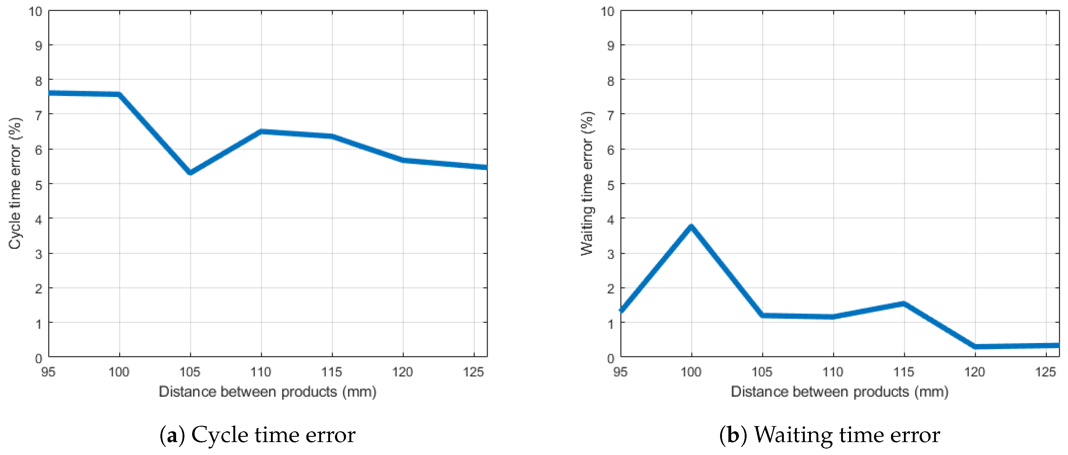
• constant distance between products: different simulations were done changing the distance between products, ranging from 90 mm to 125 mm.
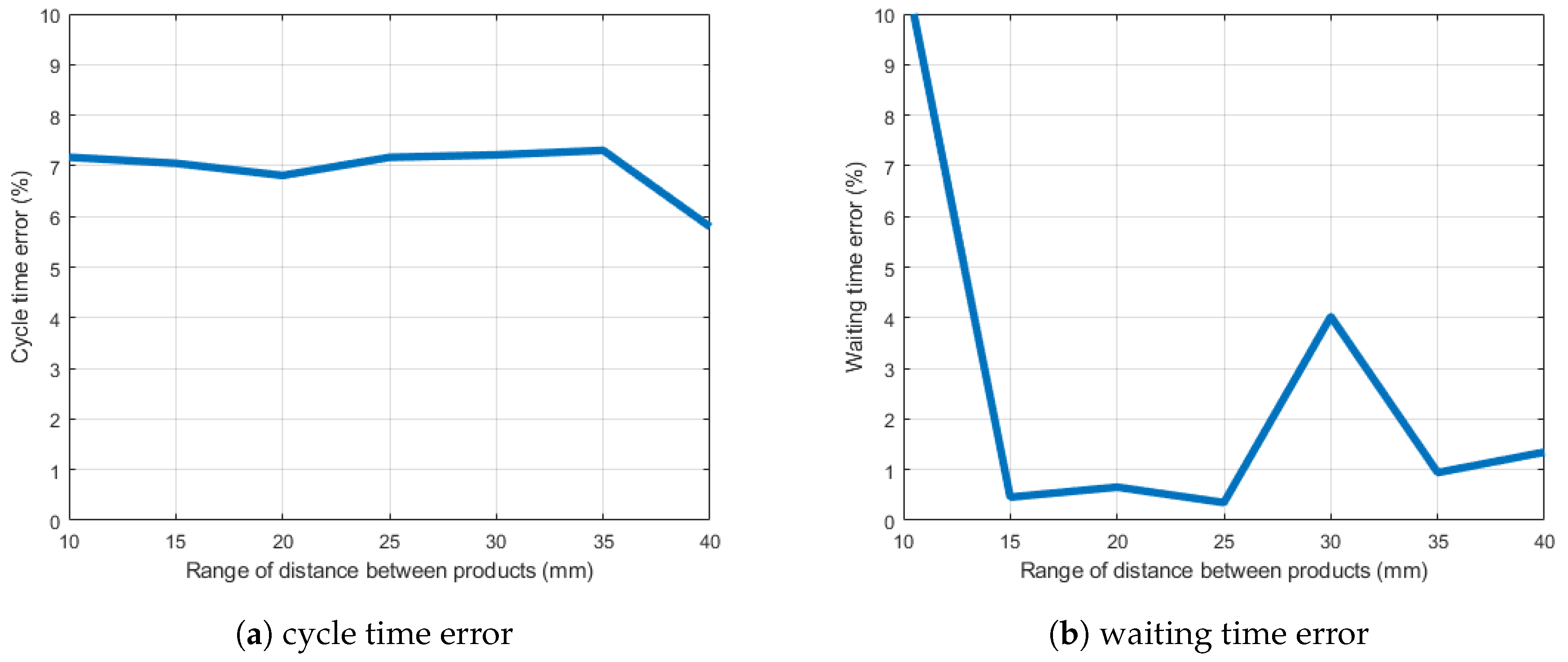
• random distance between products: different simulations are done changing the range of distance in which the product can be found. The situation evaluated ranges between 10 mm (corresponding to distances between 90 mm and 100 mm) and 40 mm (corresponding to distances between 90 mm and 130 mm).

Please note that these errors are calculated by comparing the values of cycle time and waiting time obtained using the tool developed and the Mitsubishi RT-toolbox while executing 100 pick-and-place tasks for each of the situations described. The relative graphs show the values of the error calculated. In particular, Figure 7a shows that the maximum error equal to 7.6% is obtained for the minimum distance analyzed between products. For greater distances, the error decreases. In Figure 7b the waiting time error maintains lower values and in longer distances it reaches almost zero.

In Figure 8a the error in cycle time is shown and it is approximately constant and decreases when increasing the distance between the products. In Figure 8b the waiting time error is shown and oscillates within a range of values lesser than 4%.

Taking into consideration the tests carried out in different product situations, one can note that the error is constantly maintained at values less than 8%, which is acceptable for the preliminary sizing procedure of the number of robots required in a production line for pick-and-place applications. The results obtained state that the average speed $V_{average}=1200$ mm/s, for the case under consideration, is a suitable value and can be used to calculate the number of robots required by this application.

4.3. Sizing Example

Having determined the average speed to be used in the sizing tool for the end-effector movement, one can use such tool to evaluate the number of robots required in the applications under analysis. The sizing procedure is developed making the following assumptions:

• a random distance between the products ranging from 30 mm to 50 mm
• all the robots are placed on the same side of the conveyor and the distance between them is 500 mm.
• products are aligned longitudinally, and the placing positions are defined.
• the evaluation parameter is the acceptable number of products missed according to production requirements.

The number of robots required to pick the products from the line depends on the number of products one accepts to lose. If this requirement is zero, as in the present case, the sizing tool gives a result of three robots. The tool, moreover, considers the task assignment logic of the products to the robots and the variation in distance between the products. Obviously changing these values one can obtain different number of robots required.

In the case one accepts to lose 2% of products yet maintaining the same conditions, the sizing tool produces a result of 2 robots.

Table 2. Missed products using two robots.

Simulation	Missed Products (%)
1	1.22
2	1.50
3	0.70
4	1.02
5	1.16

reports the percentage of products lost where two robots are used in five different simulations using the sizing tool and taking into account a random distribution of products (same number of pieces over a period but random distance between them, typical situation in practical industrial applications).

For every simulation there is a different percentage of lost products and the average loss in five simulations was 1.12%. Please note that by using Formula (1) 1.2 robots would have been required to pick all the products thus the use of two robots would have been more than sufficient. Instead, by introducing random variability in the distance between products (maintaining the same average product flow rate) one would require three robots to reduce the loss to zero percent.

Summarizing, the final result is obtained by adding an extra robot to the multi-robot system to guarantee the correct functioning of the pick-and-place system compared to the usual approach conventional for these sizing tasks. By using the tool developed, a different result is obtained compared to the empirical designing approach, which overlooks too many variables that characterize the system.

5. Conclusions

The sizing process of a team of robots to be used in pick-and-place applications is a complicated process in that there are a high number of variables, often unknown, depending on the robot characteristics, the production environment, and the task logic assignment of the products to the robots. This paper presents a practical method to size the number of robots required in a production line taking into consideration as many of the above variables as possible yet retaining relative simplicity. The idea at the basis of the method proposed is to use a simplified trajectory (from a mathematical point of view) and a constant travel speed of the end effector. Such speed ensures the execution of the task in the same time period as that which would be carried out by a robot in actual situations. In this way, an accurate knowledge of the robot behavior is unnecessary, and one can generalize the solution methodology to different robotic solutions and applications.

The developed tool allows one to determine the number of robots required to satisfy certain production requirements in an industrial application in a systematic and easy to use approach by taking into account boundary conditions which would otherwise be impossible to do. The sizing tool can also estimate the performance of the system helping the designer to choose the optimal combination of the design variables.

The use of the tool requires no specific knowledge of programming and can be performed in a few minutes. The behavior of a complicated industrial pick-and-place systems can be simplified by introducing the definition of an average speed easily obtainable by a simple simulation of a single station of the production line with a particular type of robot. As demonstrated in this work, the value obtained is reliable even if the distance and distribution of the products is out of the nominal data of the project. This crucial point allows one to develop a simplified model of a multi-robot scenario through which to realize a sizing tool. This tool is simple to configure with the parameters available in the early stages of the design of a production line.