1. Introduction
Unmanned aerial vehicles (UAVs) can accomplish a wide range of critical tasks in both civil and military applications. Works published in [
1,
2,
3,
4], among many others, demonstrate UAV advances that have continued to amass rapidly since the turn of the century. Miniaturization and mass production have enabled the use of multiple small aircraft to accomplish missions that were previously only possible with large, expensive vehicles [
5]. Small UAVs have a short mission life due to limited on-board power, thus diminishing their utility to accomplish a sustained task. This paper presents a persistent retrieve, recharge, and redeploy algorithm that enables a group of small quadrotors to search and track moving targets in a defined space.
Considering the limitations of current battery technology, increased endurance of a group of autonomous agents must rely on some form of coordinated recharging. An integrated robotic systems approach that automates the retrieval, recharge, and redeployment process may satisfy this need. The recharging process must sustain multiple agents beyond the flight endurance of a single agent. For a group of agents to accomplish a prescribed task, recharging must be coordinated with long-term task execution. By incorporating an automated replenishment procedure, a group of agents can persistently complete an assigned task. This paper presents a replenishment procedure that sends agents with a low battery to a recharging station; agents that are fully charged are launched when necessary, and the group continues accomplishing the mission. This concept increases the overall endurance of the group’s data acquisition capabilities (video, acoustics, spectral, etc.), and the area of operation.
The existing literature related to UAV technology and its applications is extensive. We focus here on works addressing persistent multi-vehicle systems and multi-agent search and track algorithms. The authors in [
2] created a system of four aerial agents capable of executing a sustained task. Their replenishment system is an automated battery hot-swap that mechanically changes depleted batteries to refuel aerial assets. In this work, we consider a larger group of smaller UAVs that are captured for recharging rather than swapping batteries. To do so, we employed methods from [
5] which enable the control of coordinated maneuvers for up to 50 Crazyflie 2.0 quadrotors.
Several works have also demonstrated autonomous replenishment methods: [
6] used induction coils on a landing platform; [
2] utilized a custom-designed battery swapping mechanism interfaced with a landing structure; and [
7] proposed the use of a robotic arm to capture and place agents into a recharging structure to reduce the environmental uncertainty associated with precise landing. Like [
2,
6,
7], we assume that any replenishment method is accomplished at a known, stationary home base location. In related work, [
8] presented an autonomous system of delivery robots that provide charged batteries to robots completing an assigned task.
A significant number of works have investigated multi-vehicle search and track applications while assuming unlimited vehicle endurance [
9,
10,
11,
12]. In [
9], the authors implemented a recursive Bayesian estimator to detect and track targets by continuously updating a likelihood measurement of target presence. The authors of [
12] used a similar detection and tracking technique to switch vehicle behaviors according to motion governing states of matter. Vehicles searching for targets move rapidly, a gaseous state; vehicles detecting targets slow down as they approach the target location, a liquid state; and vehicles hovering at target locations have very little motion, a solid state. This paper builds upon these search and track methods by accounting for limited vehicle endurance.
The central focus of this work is to achieve a reliable algorithm to direct multiple vehicles for a coordinated task for an extended period of time, i.e., longer than a single battery cycle. The concepts presented in this work are intentionally generalized to allow application to a variety of multi-agent systems. Integration of multiple agents into a cooperative task requires the continuous monitoring and analysis of battery status, task assignment, trajectory assignment, trajectory evolution, and collected data.
With this in mind, the goal of this work is as follows: derive an autonomous multi-vehicle control algorithm coordinating vehicle motion to persistently search for and track targets in a defined area subject to the endurance constraints of individual agents. The contribution of this paper is an algorithm that can (1) control multiple UAVs to search trajectories in a given space, (2) plan around the limited flight time of each vehicle in the search planning process, (3) track targets that are found on search trajectories, and (4) persistently monitor the specified domain. The algorithm must account for the appearance, motion, and disappearance of multiple targets in the search space. When tracking, UAVs maintain position over a target as it moves about the search domain. When the battery level of a vehicle drops below the predetermined threshold, the agent must return to charge. Remaining agents must account for the loss and gain of agents as they exit and re-enter the search environment.
The remainder of the paper is organized as follows.
Section 2 presents the persistent multi-agent search and track algorithm;
Section 3 presents simulated and experimental results; and
Section 4 provides closing remarks and offers directions for future work. The small-scale experimental system results in this paper serve as proof of concept of the algorithm’s viability in operational environments.
2. Approach
The proposed algorithm consists of a high-level, heuristic decision-making process that assigns agents to different operational modes. This section presents the algorithms comprising each mode of operation, along with the sensing and monitoring algorithms that regulate switching between operational modes.
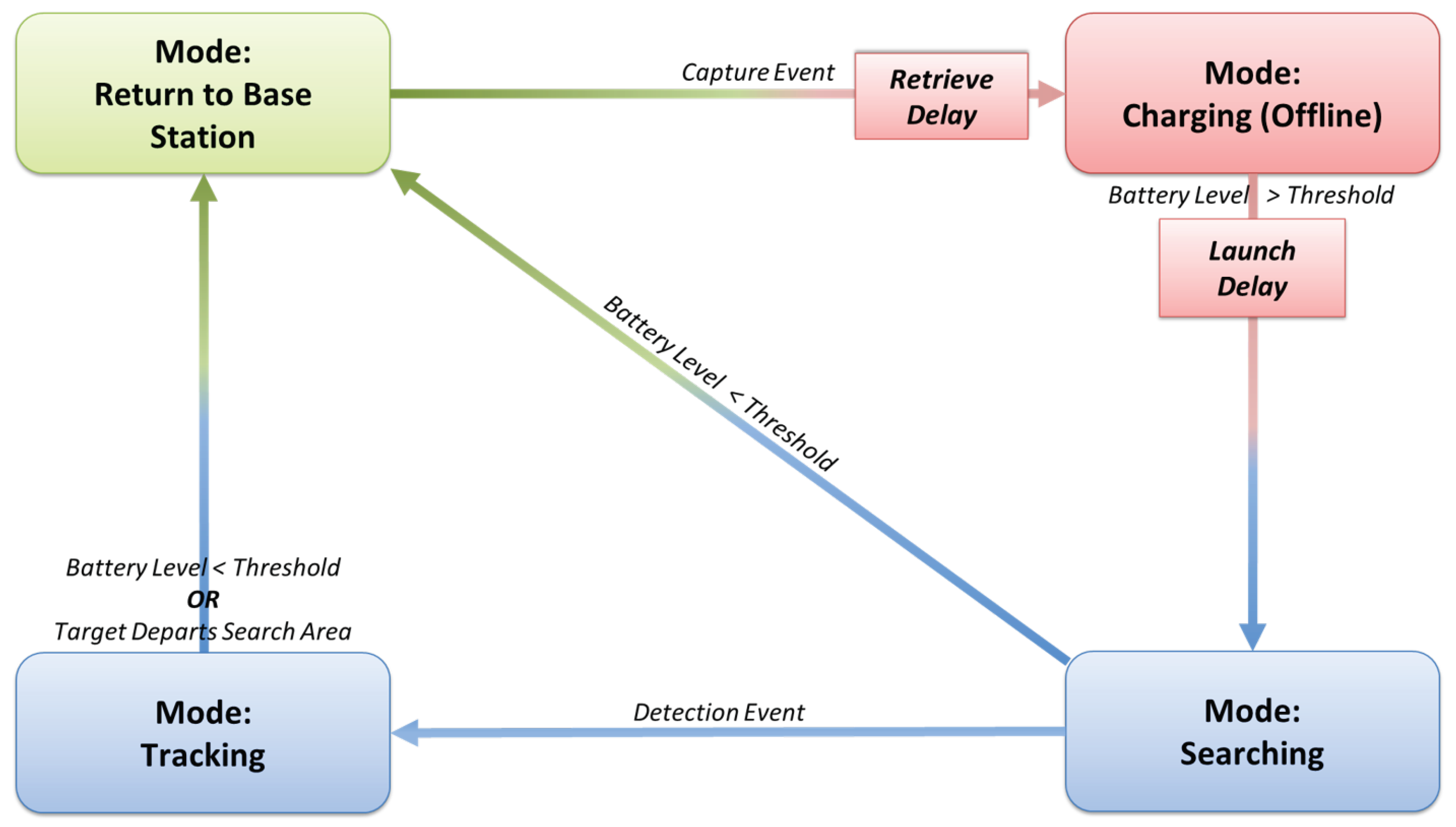
Figure 1 offers a visual representation of the control algorithm modes and their corresponding triggering events. The algorithm is composed of four operational modes, including search, track, return to base, and charging/offline. Each block represents a different operational mode, with the arrows denoting events that trigger a mode transition. The remainder of
Section 2 is organized according to each of these modes. The general operational cycle starts with the agent launching into search mode, shifting to track mode if the agent finds a target, returning to home base to recharge when the battery level is below threshold levels, and ending with a recharging phase.
The search and track task modes are inextricably linked. Search mode consists of a trajectory prescribed to each agent and is the default mode when a vehicle is launched. Track mode is triggered by a detection event prompting a UAV to follow the identified target. Return mode is triggered when an agent’s battery drops below a designated threshold. In return mode, the agent guides itself to the base station to recharge. Recharge mode accounts for the recharging period, wherein the agent is offline and no navigational or sensing computation is needed. This mode is triggered by a docking event with the recharging station following a delay associated with the time required to capture an agent. When a charging vehicle’s battery level exceeds a specified threshold, it is marked as available, and the cycle can repeat. Note that available agents can continue to charge until they are needed. The launch and retrieve delays are motivated by the autonomous recharging system presented in [
6,
13]. Our work assumes that vehicles default to search mode immediately following launch. This is a possible limitation that is the topic of ongoing research.
2.1. Mode: Search
The search task requires agents to cooperatively monitor the defined region in space and time. This paper uses smooth space-filling curves to explore defined subregions of the domain. Each curve defines a desired search trajectory that is used to calculate a prescribed vehicle speed and direction along the curve. This section derives the desired search trajectories for each vehicle using a differentiable piecewise function of time. A large body of research exists on optimal search trajectories for multiple agents using different mathematical strategies [
9,
10]. Without loss of generality, this work relies on simple space-filling curves.
Each agent’s trajectory defines a desired position, velocity, acceleration, and yaw angle with respect to time. Trajectory generation is divided into the following steps: (1) define a numbered set of positions in the search space, (2) calculate a differentiable piecewise polynomial that connects the positions, (3) parameterize the piecewise polynomial with respect to the path frame variables, and (4) relate the path frame coordinate to time using a scaling relationship that ensures that agents travel at a constant, desired speed.
2.1.1. Search Path Generation
Given a bounded subregion within the search domain, an ordered set of three-dimensional points in space can be used to define the desired points on a search agent’s path. This section details the methods to define the ordered set of points and the continuous piecewise polynomial that defines the path. Defining the ordered set of points relies on two key assumptions: (1) each vehicle has a sensing field-of-view described by a cone oriented downward relative the UAV’s coordinate frame; and (2) each vehicle maintains approximately level flight such that the sensing cone’s projection onto the ground is a circle of radius
r for a fixed altitude
h. Under these assumptions, the grid of points is separated by
to avoid overlap in coverage. Using these points, the path is composed of an alternating series of straight segments and coordinated turns with a radius equal to the sensor radius. To prevent searching outside the prescribed space, subregions are offset using the simulated sensor radius. The resultant points consist of an
position and are numbered by order of visitation. The UAV path
is defined as a function of the continuous domain
given a set of
n points such that
is the first
X coordinate in the ordered set,
is the second, etc. Gaps between integer values of
s are defined using first-order polynomials for straight sections and fifth-order polynomials for the curved sections.
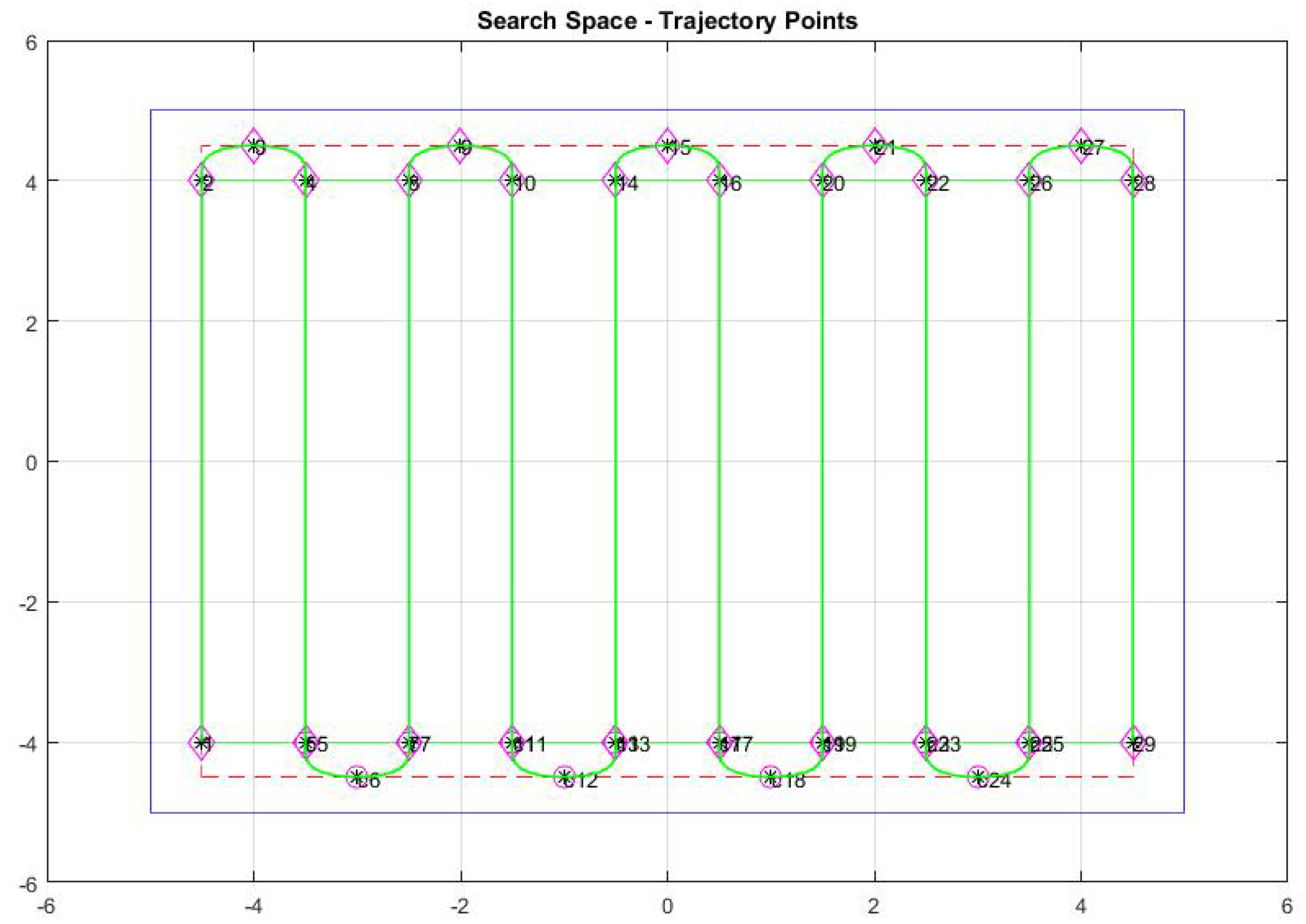
Figure 2 visualizes a rectangular search domain where the numbers near each point define the point’s designation in the path frame variable
s. Curved sections are uniquely defined using constraints on the position and tangent at the start, apex, and endpoint.
The fifth-order polynomials for
and
are defined by
where the constants
through
for
and
are calculated using the method described in [
7]. Straight segments are first order, with only two endpoint constraints. Coefficients of these polynomials are calculated similarly [
7]. Note that
is set to a constant height
without loss of generality. Setting the desired height allows for altitude collision avoidance by placing agents in different modes at different heights to minimize the chances of collision.
2.1.2. Temporal Execution of Polynomial Trajectory
Given the paths defined as a function of the path frame coordinate
s, the vehicle trajectory is prescribed by establishing the time-dependent function
to impose a constant speed along the path. Using this definition, velocity is
since
is constant and speed is
Given a fixed desired speed
, setting
gives a differential equation governing evolution of
Subsequent derivatives of Equations (4) and (8) provide the acceleration along the path, but they are omitted for brevity.
2.1.3. Trajectory Implementation
Each agent trajectory is implemented using the piecewise polynomials that characterize the position
, velocity
, acceleration
, and yaw
. The desired trajectory vectors in terms of
and associated derivatives are defined by
Figure 2 shows an example of the resultant pattern in a rectangular search space using Equations (9)–(13), where the green line is the desired path and the red and blue lines illustrate the search boundary offsets.
Fully defined trajectories are tracked using the quadrotor trajectory controller derived in [
14]. The controller calculates the error between the desired position and orientation and returns motor thrusts to achieve the desired path. The controller allows for the assignment of the desired position, velocity, acceleration, and yaw angle, all of which are translated into control inputs. We rely on this control for the launch and return phases of the trajectory by similarly defining straight line trajectories to the respective desired endpoints.
2.1.4. Multi-Vehicle Planning
In order to best allocate the agents to the search region, the algorithm must assign each agent to a unique search area. Here, we present a partitioning algorithm used to define search regions for each agent. We partition the search space using the nominal flight speed , flight endurance , and sensing radius r at altitude h. Over the course of a battery life cycle, an individual vehicle can search, at most, square units. Allowing additional battery usage for return and a general safety factor, we uniformly partition the space into regions of area , where designates the safety factor. For simplicity, the results in this work assume the partitions are constant throughout the mission. Ongoing work seeks to dynamically repartition the space to focus on undersampled regions.
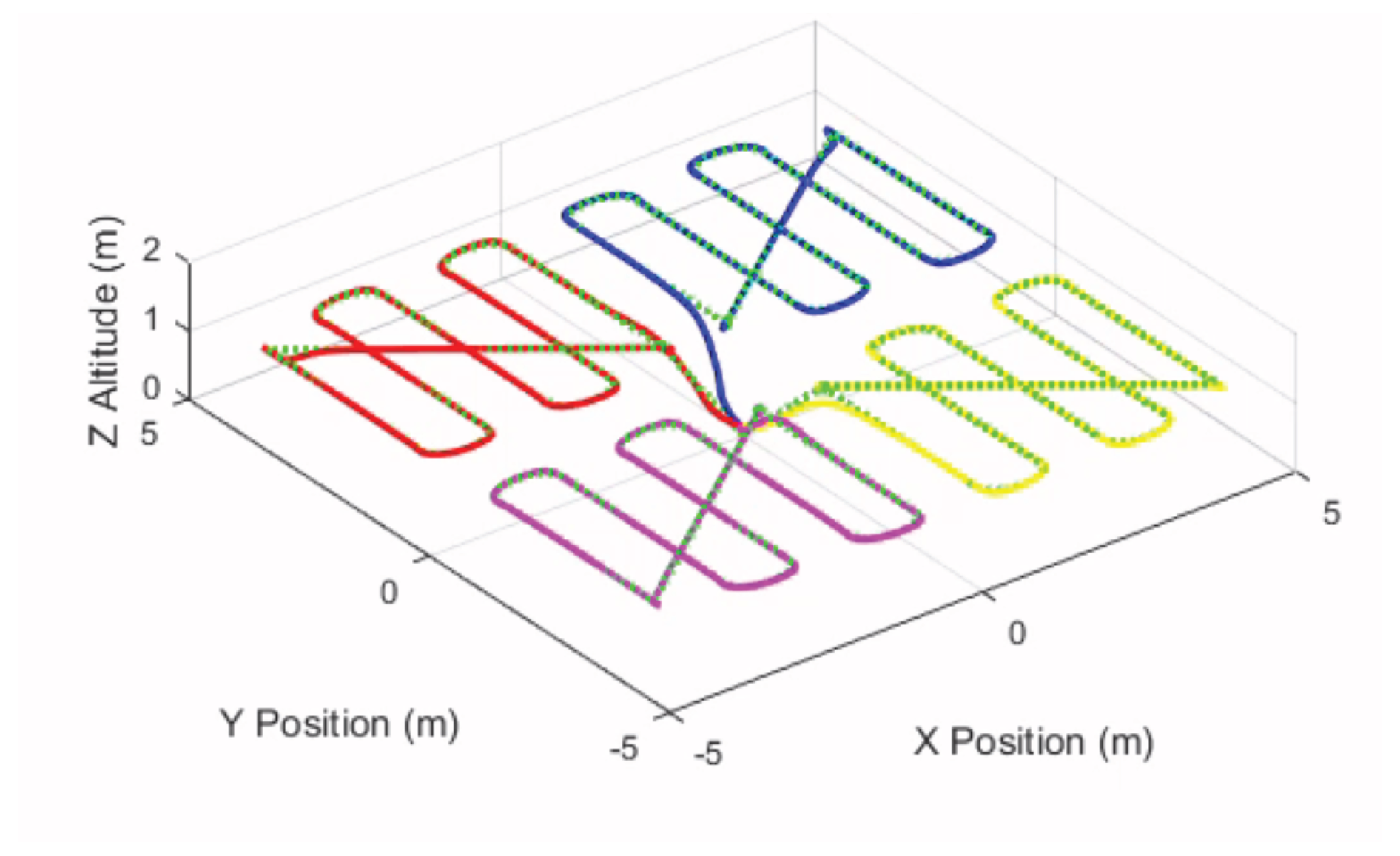
Figure 3 illustrates a simple partition showing four equal quadrants. The results of
Section 2.1.2 and
Section 2.1.3 subsequently enable trajectory generation within each quadrant. The dashed lines in each quadrant indicate the desired trajectory, whereas the solid lines show the simulated trajectories of the quadrotors using the trajectory tracking controller [
14].
2.2. Mode: Track
Target detection is the triggering event that transitions an agent from search to tracking mode, and it is accomplished using a likelihood ratio tracker [
12]. This section provides a summery of the sensor measurement assimilation procedures used to indicate detection events. We assume a generic conical sensor projection onto a two-dimensional plane resulting in a circular or elliptical footprint. A conical projection approximates devices such as thermometers, infrared sensors, or radiation detectors without loss of generality. The conical sensor field of view (FOV) is projected onto the ground plane of the search space, returning simulated scalar measurements within the area of intersection of the cone and the plane.
The detection step leverages likelihood ratio tracking techniques for the detection and tracking components of the control algorithm. Work published in [
10,
12,
15] detail the use of likelihood ratio tracking (LRT) to detect targets; we provide a summary here for brevity. This detection technique associates sensor measurements with a probability of target presence and creates a ratio of likelihood of target presence to likelihood of target absence [
12,
15]. When the ratio exceeds a predetermined threshold value, a detection occurs. Specific details regarding derivation and implementation of the algorithm are provided in [
12,
15].
When the likelihood ratio tracker detects a target, the vehicle switches from search to track. In track mode, we assume the vehicle estimates the position and velocity of the target in its field of view. The estimated target position and velocity are used in the trajectory controller [
14] such that the quadrotor follows the target as it moves through the domain.
2.2.1. Target Motion Model
We assume targets move randomly through the search space. The model includes constraints to give the targets a realistic motion pattern, as they are constrained to reasonable heading shifts and speed changes; therefore, they cannot instantaneously reverse their speed or heading. Targets update their heading and speed at random time intervals such that they travel along a piecewise continuous path of straight line segments. Targets’ speeds are bounded between and m/s, and each target’s heading is bounded within rad of its heading from the previous segment.
2.3. Mode: Return
To extend the operations of the multi-vehicle team beyond the battery life of a single vehicle, the algorithm must incorporate return to base and recharging requirements. The return mode uses the piecewise polynomial approach discussed in
Section 2.1. Once set to this mode, the algorithm takes the current
location of the agent and the known home base point and calculates a straight line path between the two. The return path vector is defined by
, where
is the start point, the current location of the agent, and
is the endpoint, the known home base location, of the return path. The return path is defined by
,
, and
, for some altitude
deconflicted with the search altitude. The
X and
Y components of the trajectory are evaluated using the same method described in
Section 2.1.2 and
Section 2.1.3. Altitude,
Z, remains constant. Once the agent reaches the base station, it is switched into recharging mode. The transition to recharge is dependent on the recharging mechanism implemented.
2.4. Mode: Recharge
After a vehicle returns to base, it enters recharge mode. During this time, the agent is marked offline and charges until it has a full battery. The battery charge and discharge behavior are based on the nominal flight characteristics of the CrazyFlie2.0 [
16] quadrotor. Through experiments, we verified a mean flight duration of 7 min and a mean recharge time of 20 min.
Battery models are generally nonlinear and can be unique to the individual battery chemistry and capacity. Additionally, factors such as charge cycles, voltage draw, and ambient temperature can have a significant impact on the effective battery capacity and discharge rate. Since the goal of the present work is to schedule recharge and redeployment of a group of agents, the most important characteristic of the battery behavior to capture is the flight time and recharge time. To these ends, we implemented a simple battery discharge model that assumes that the charge decreases linearly over time while the vehicle is in flight. The battery model used in the simulations is
where
is the battery level (in percent remaining).
is the battery state at the time of transition, and
such that the battery discharges faster than it recharges. One can manipulate the discharge and recharge time by modifying
and
. The parameters of the discharge model are chosen conservatively such that the battery is at 25% capacity after 7 min of flight. The charge model is also linear with time, and the parameters are chosen such that a vehicle can charge from 0% to 100% in 20 min. A full agent cycle is defined as 7 min of flight time followed by 15 min of recharge time, an approximately 1:3 flight-to-recharge ratio. While a 1:3 flight to recharge ratio is slightly unrealistic for a small UAV platform, this ratio can be attained by larger UAVs with higher capacity batteries and chargers. It should be noted that the algorithm presented here is agnostic to the specifics of the battery charge and discharge models, although the simulation results should be interpreted with that in mind.
2.5. Multi-Vehicle Coordination
The primary goal of this algorithm is to coordinate multiple vehicles in a search and track task. We approach this problem by assigning states to each agent describing their role in the group. The assigned states for each agent include a vehicle identifier, its search cell, its mode current designation, its elapsed time in the latest search or track mode, and its battery level. The algorithm determines the search assignment and mode transitions based on the evolution of these states in time.
The general priority of mode assignment is to ensure a deployed agent has sufficient battery to search, track detected targets, and return. The goal of the search assignment is to assign available vehicles to cover all search cells to agents. This objective is achieved using a heuristic decision-making model. The strategy rules are as follows. Agents are deployed only into search mode. After deployment, the vehicles only communicate with the base if a target is found or if returning to charge. As such, the home base tracks the sequence of search zone deployments and assigns newly deployed agents to the highest priority zones. The highest priority zones are determined based on the previous deployments, time in search/track mode, and information received as vehicles return. Search cells are tracked and assigned to a single search agent, since they are created for the intention of a single agent to cover the entire area effectively. No agent tracking a target will be set to a mode other than return, and we assume that agents communicate sensor readings to their neighbors to prevent two vehicles from tracking a single target. The search, return, and track modes are altitude deconflicted by allocating vertical sections of airspace to each mode and a priori assigning an altitude to each agent operating in that mode.
3. Results
In order to validate the the performance of the algorithm, a series of simulations and hardware experiments were conducted.
Section 3.1 describes the metrics used to assess the algorithm’s effectiveness in coordinating the multi-vehicle system for searching and tracking targets in the space and the overall usage of available vehicle assets.
Section 3.2 summarizes results from over 70 simulations of the persistent multi-vehicle search and track algorithm to analyze the relationships between the number of agents, targets, and domain size.
Section 3.3 summarizes the results of hardware experiments using crazyflie quadrotors and ground vehicles.
3.1. Coverage, Tracking, and Vehicle Usage Performance Metrics
In order to evaluate the performance of the multi-vehicle search and track algorithm, we utilized three metrics. The first metric measures the coverage of the search area in space and time. In the ideal case, the entire search area would be covered for the entire duration of the task; this would constitute 100% coverage. In light of the reality of the coverage problem, the goal is to maximize the detection of targets by maximizing the coverage over the duration of the task. We divided the search region into equal-sized quadrants and assigned a scalar value
to the
ith cell to measure coverage. The coverage value decays linearly when a sensor field of view does not cover it, while it is maximal when covered by a vehicle such that
where
is the linear decay constant corresponding to the temporal scale of measurement validity, and
without loss of generality. We define the mean coverage as the average coverage value over the entire domain.
The second metric measures tracking performance as the number of targets tracked given the number of total targets in the scenario. The final metric used to determine algorithm performance is vehicle usage. Vehicle usage measures the number of agents deployed relative to the number of total agents in the group.
3.2. Simulation Results
Here, we present the results of simulations with varying quantities of agents and targets. We varied the number of agents between 4 and 12 and varied the number of targets between 1 and 3. Each simulation assumed a 1 h search and track mission.
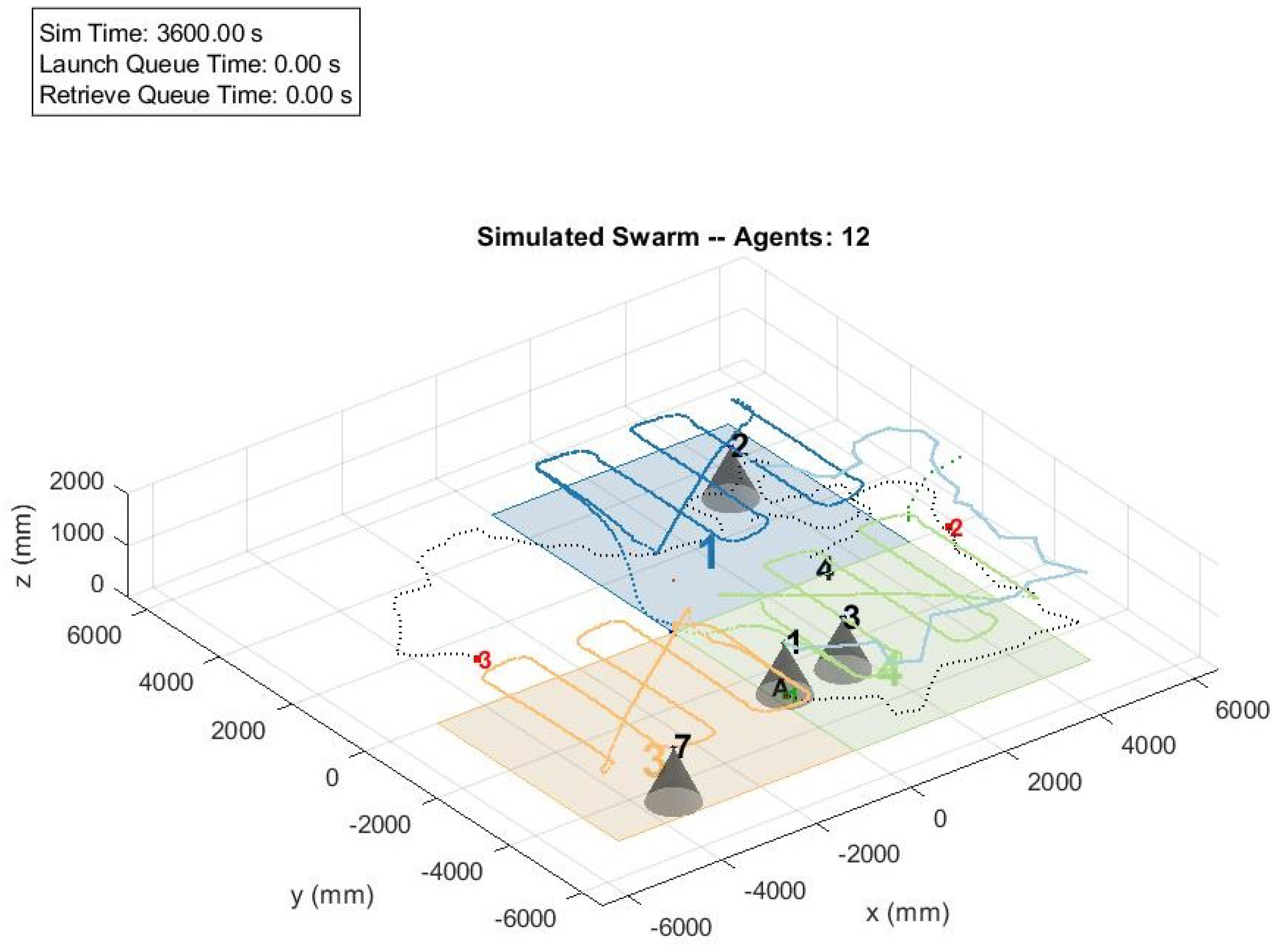
Figure 4 is a visualization of an example simulation operating with 12 total agents searching for 3 random targets. The black numbers indicate search agents, with light gray denoting sensor cones. The red numbers are untracked targets and the black letters are tracked targets; positions of all simulation elements for the previous minute are illustrated by dashed (targets) and solid (agents) lines. The color patches are search cells occupied by agents assigned to the search mode. Note that at this particular time in the simulation, agents 1, 2, 3, and 7 are deployed, whereas the remaining are either charging or in queue for deployment. The figure illustrates the complexity of the multi-vehicle mission.
Simulations include 4, 6, 8, 10, and 12 agents searching for 1, 2, and 3 targets in all combinations. The following discussion focuses on the case of 4 and 12 agents searching for 3 targets because their greater disparity is conducive to comparing results. Note that the figures using blue lines indicate simulation results with 4 agents, whereas red lines indicate simulations using 12 agents. These simulation results represent the aggregation of over 70 simulations.
3.2.1. Coverage Results
Figure 5 and
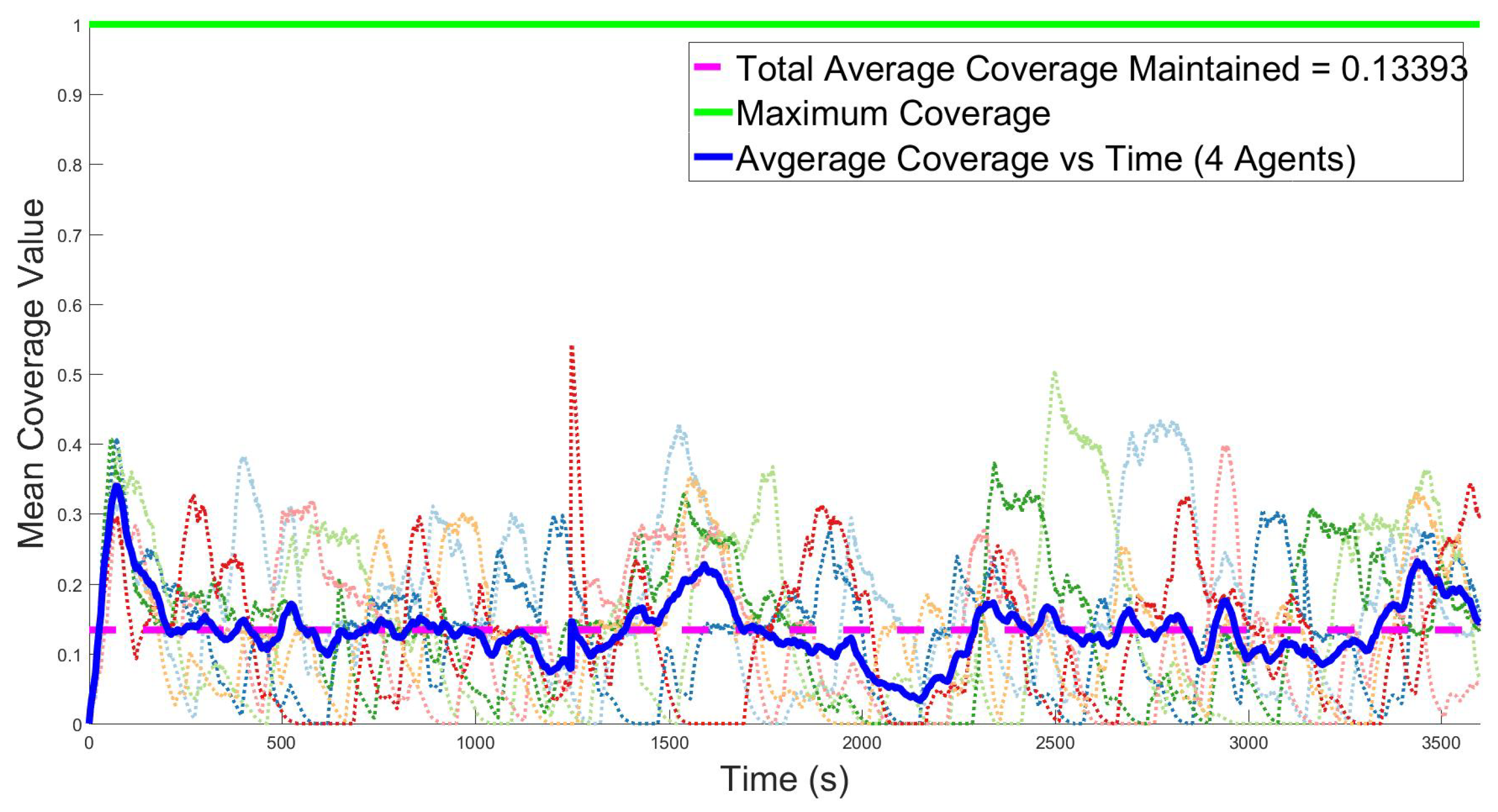
Figure 6 show the average coverage value for the search region over time. The light colored dotted lines are the values for individual simulations, the green line is the maximum value, the solid line is the average for all trials over time, and the dashed magenta line is the overall average of all runs and all time. Recall from
Section 3.1 that the ideal case is the maintenance of 100% coverage for all time, which equates to 0 seconds since the last revisit. In
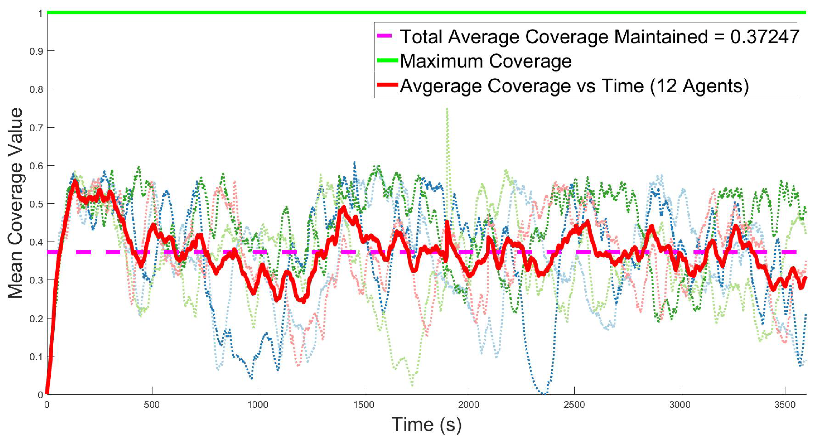
Figure 5, the average coverage value, approximately 0.13, corresponds to 43 s since the last revisit averaged across the entire search space. In the 12-agent case, the average value hovers near 0.37, as shown in
Figure 6, corresponding to 32 s since the last revisit. As shown in the figures, the general coverage value tends to increase as the number of available agents increases.
Note that in each of the figures, the coverage spikes before any targets are detected. Then, the coverage drops closer to the mean value as agents need to be removed from service for recharging. This trend suggests that the maximum coverage value for that agent case is the initial spike, and further improvements in the swarm task assignment algorithm can raise the average coverage value closer to this maximum value. Momentary lapses in coverage (i.e., 0) occur when the group’s overall battery levels are depleted such that all vehicles are returned to charge or that all deployed vehicles are tracking targets. As expected, the 12-agent case sees fewer lapses in coverage since more assets are available.
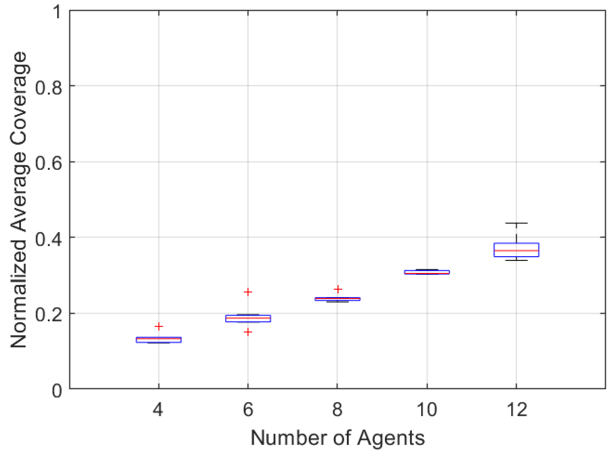
Figure 7 illustrates coverage trends for the three target experiments and an increasing number of agents. The box plot shows an increase in average coverage as the number of agents increases. As expected,
Figure 7 shows increasing coverage as the number of agents increases.
3.2.2. Tracking Results
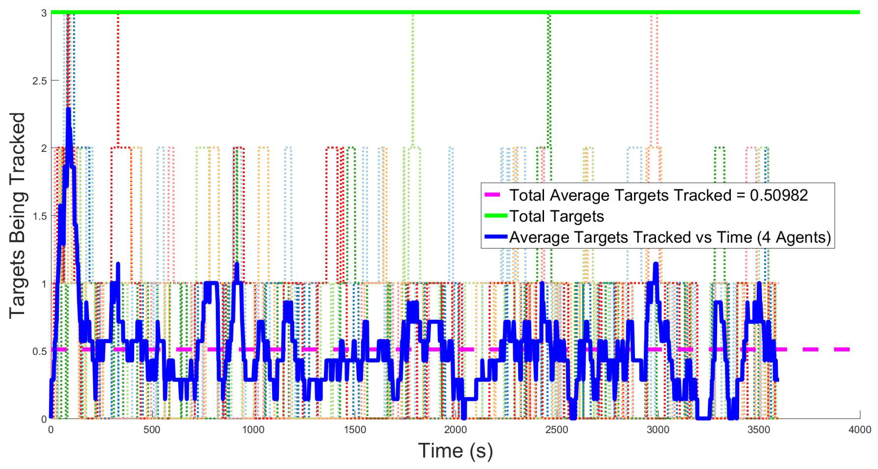
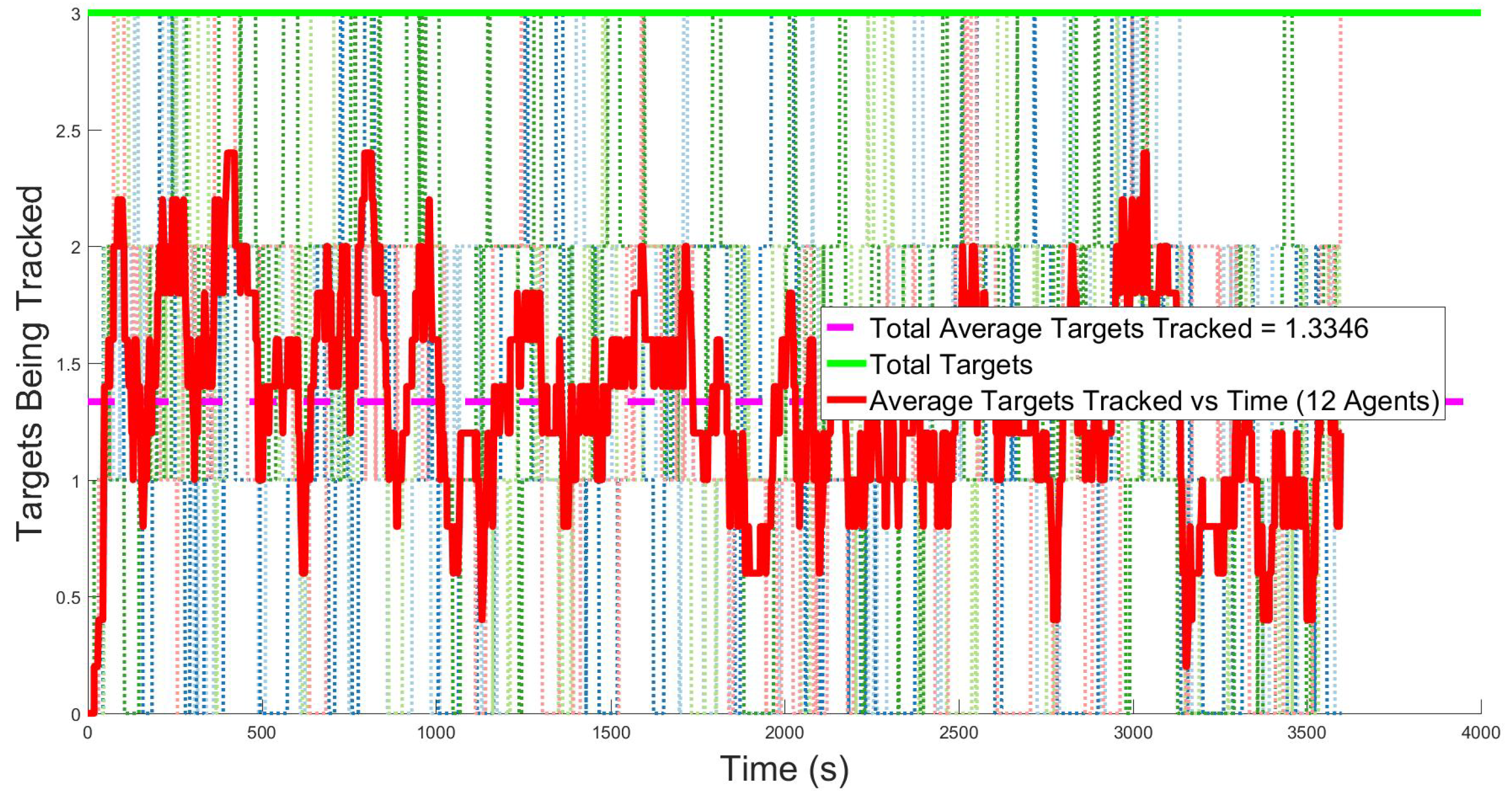
Figure 8 and
Figure 9 describe the overall tracking performance of the group over time. Light colored dotted lines illustrate individual experiments, the green line shows the maximum number of targets (three, in the figures shown), the solid line is the average for all trials over time, and the dashed magenta line is the overall average of all runs. However, as shown in the figures, having more agents available results in more targets being tracked, an expected outcome.
Figure 8 shows 4 agents are able to track 0.5 out of 3 targets on average.
Figure 9 shows that, on average, 12 agents are able to track nearly 1.5 targets for all time.
Notice that no matter the number of agents, there is a large degree of variability in the number of targets tracked from experiment to experiment. This is caused by the method used for resetting targets when they leave the search space. The targets walk randomly through the space and are reset to a new location if they move beyond the search space boundary. The target reset effectively acts as a lost target, even though the agent may still have the ability to continue tracking. Alternative approaches to modeling target behavior include settings in which the target always remains within the search region or a new target is spawned at the edge of the region when another target leaves the search space. Each of these approaches would result in different coverage performance and would be appropriate depending on the specific use case of the algorithm.
3.2.3. Vehicle Usage
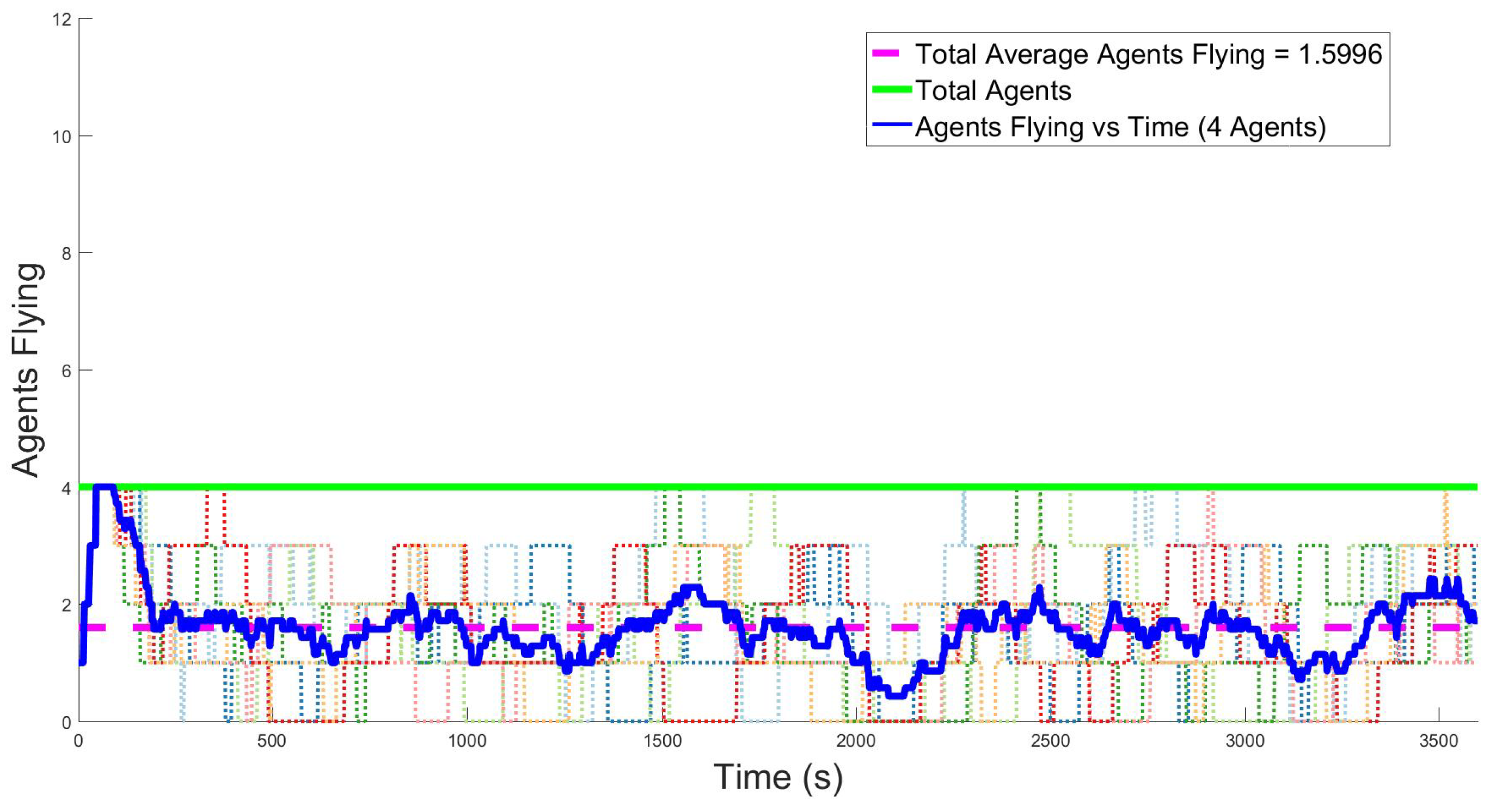
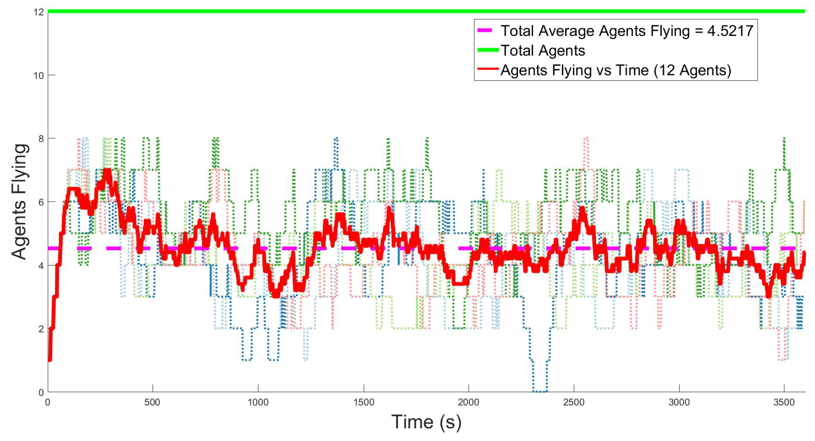
Figure 10 and
Figure 11 show the overall vehicle usage as a function of time. The light colored dotted lines are the values for individual experiments, the green line shows the maximum number of agents available, the solid line is the average for all trials at that time, and the dashed magenta line is the overall average of all runs. This metric is intended to measure the effect that recharging has on the operation of the group. The ideal case is to have the maximum number of agents flying. However, given the search area and number of targets, there may be fewer than the ideal number of agents needed. As shown in the figures, more available agents imply more agents are airborne on average, an expected outcome of adding more agents to the simulation. In
Figure 10, of 4 available agents, approximately 1.5, on average, are airborne throughout the whole experiment.
Figure 11 shows that when increasing the total number of agents to 12, an average of nearly 4.5 agents are airborne over all simulations. In both of these cases the average number of agents airborne is 37.5% of the total number of agents.
The battery status for each of the agents directly relates to the usage metric because recharging is the highest priority operational mode. Any agent will drop its task to go recharge if needed, regardless of the task it is accomplishing. Each agent completes approximately three battery life cycles over the course of a 60 min experiment. Overall, the increase in average usage as the number of available agents increases is a numerical validation of the expected behavior of the group and motivates investment in having the ideal number of agents.
3.3. Experimental Results
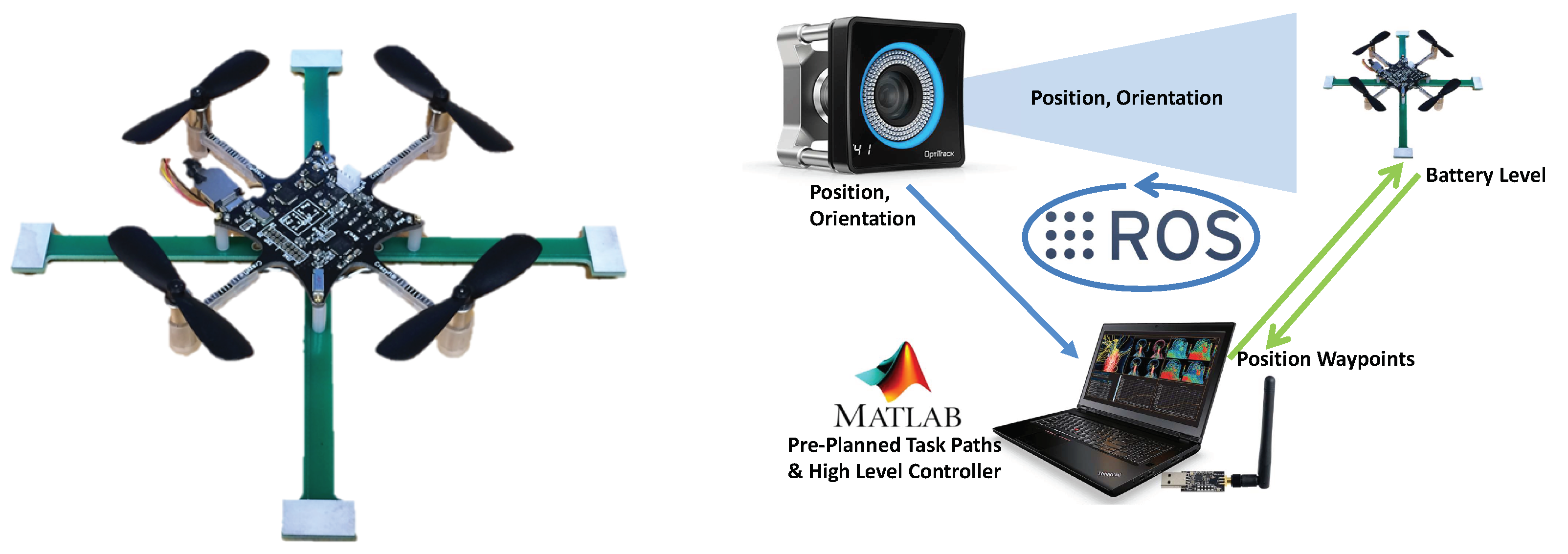
To further validate the methodology, a series of hardware experiments were conducted. The experiments were conducted in a 5 m × 6 m work space. A motion capture system was used to provide position feedback of the agents and the targets. We assume that, in an applied implementation, vehicles are outfitted with a sensor suite capable of providing position information such that motion capture is not a limiting factor. The experimental platform used for the agents was the Crazyflie nano-quadcopter shown in
Figure 12(Left). The targets were teleoperated radio-controlled cars with tracking markers. The target vehicles were driven by human operators who were instructed to randomly drive the target vehicles throughout the workspace. This approach emulates the random motion of the targets in the simulations without loss of generality.
Robot Operating System (ROS) was used to implement the communication structure between the various components of the experiment.
Figure 12(Right) shows the ROS communications between the MATLAB node and the agents in green arrows and the ROS rigid-body messages from the OptiTrack System to the MATLAB node. Using this architecture, the data were shared between the computer controlling the flight controls of the UAVs and the computer running the algorithm. The approach to controlling multiple Crazyflies simultaneously was derived from the work presented in [
5]. The centralized multi-vehicle search and tracking algorithm was implemented as a software node in MATLAB. The centralized algorithm listens to the positions of the targets and agents, as well as the battery level of the agents, to execute the persistent search and track task. The sensor cones were simulated by the computer using position and orientation data from the motion capture system.
A key contribution of the hardware experiments is the use of the voltage levels measured from the actual UAV instead of a simulated battery model. This is an important distinction since the battery discharge is not as deterministic as the simulated model and can have significant variations between specific vehicles. We set voltage thresholds to maximize usable flight time and provide realistic mission life constraints to hardware experiments. Experiments replicated recharging by launching new UAVs from a charged queue, effectively employing nearly twice the agents needed to conduct an experiment with an autonomous recharging platform.
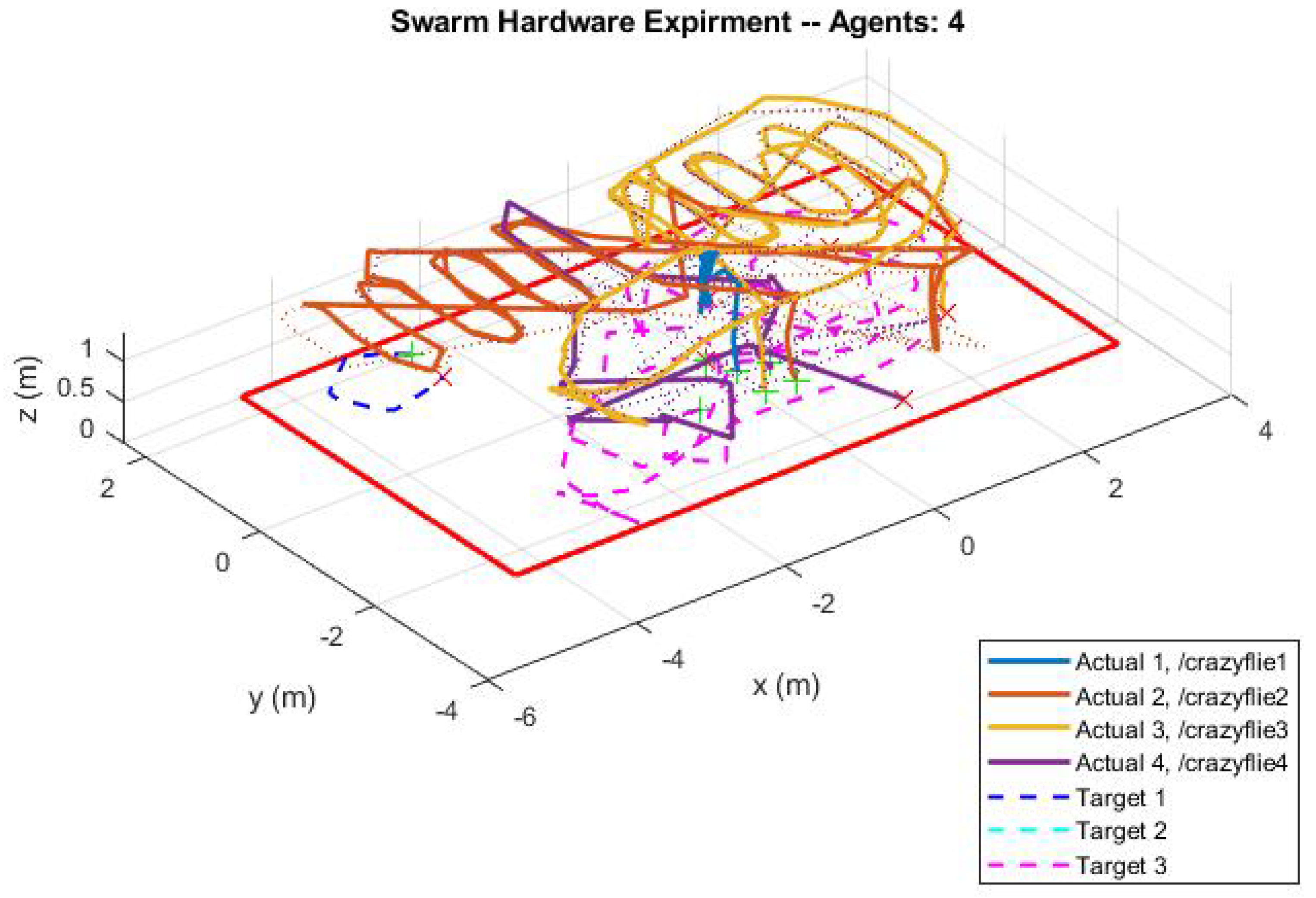
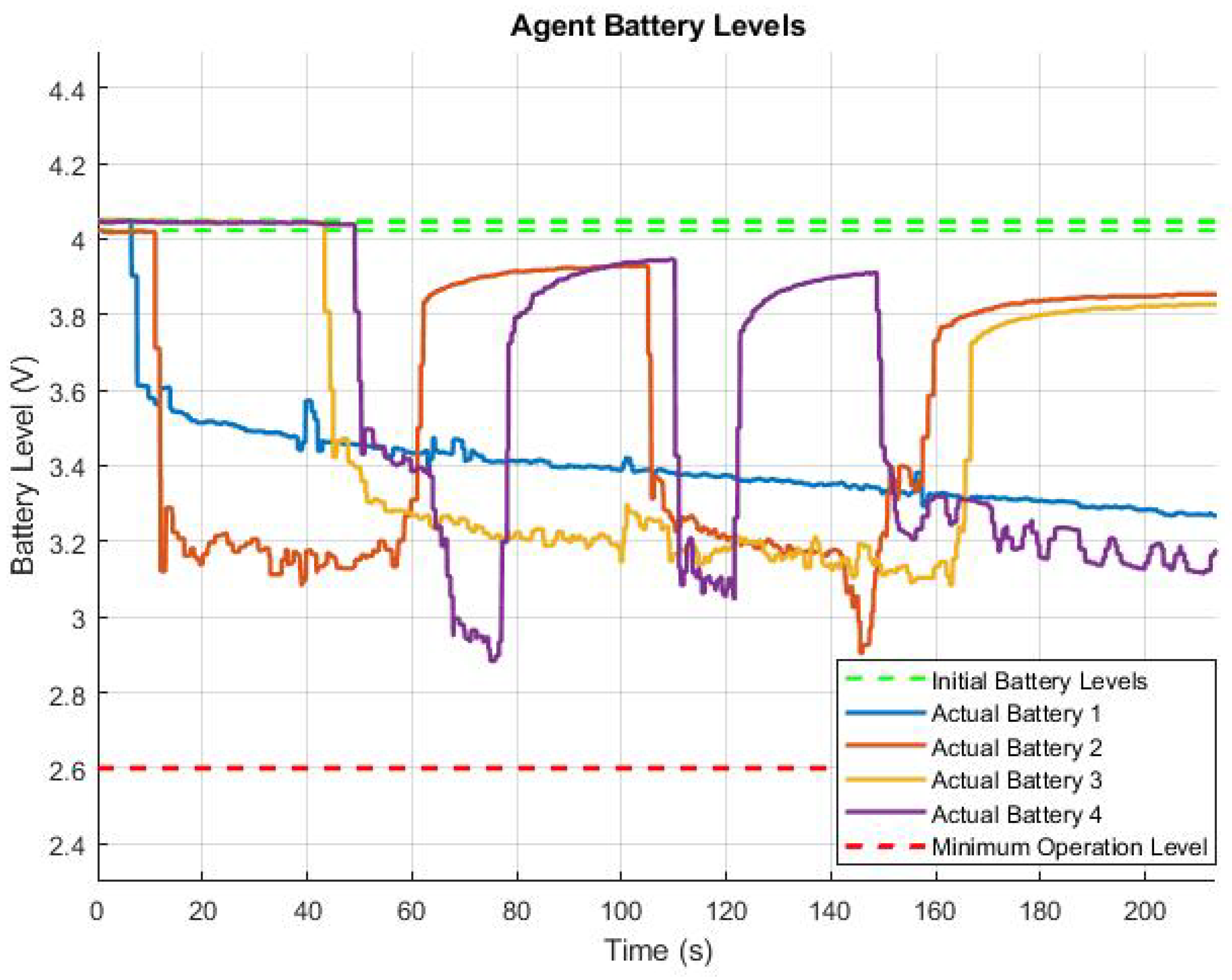
Figure 13 visualizes the totality of a four-agent, three-target experiment. The colored lines denote paths traveled by agents and targets, and the red box signifies the search boundary.
Figure 14 shows the battery levels over the course of the experiment. Note that large oscillations occur when an agent lands and relaunches during the experiment. One of the challenges associated with the hardware experiment was determining the robust operational voltage thresholds caused by variability between individual UAVs. In this experiment, we were able to demonstrate that each of the operational modes functions properly. An agent successfully completes a search path, as shown by the coordinated red and orange paths on the top of the figure. An agent successfully detects and tracks a target, as seen in the the random paths throughout the figure. Finally, an agent successfully returned to home base for recharge, evidenced by the oscillations in the red and purple lines in
Figure 14. This experiment demonstrates that the algorithm discussed in
Section 2 is capable of directing a multi-vehicle mission with actual UAVs.
While this work utilizes a centralized form of autonomy for development and testing, the concepts presented here could be extended to a decentralized autonomous platform that allows agents to make tasking decisions for themselves. This could be further developed to include sensor measurements taken directly from the vehicle, although that would require a larger, more capable UAV platform.
4. Conclusions
This work presents a multi-vehicle control structure that addresses the limited battery life of individual agents to accomplish a persistent search and track mission. The control structure maps the relationships between control modes to increase the overall ability of a multi-vehicle team. This approach allows for scalability to different assets or tasks. To accomplish the search and track mission, we designed search trajectories to enable reliable coverage of the entire search space. To enable persistent operations for realistic platforms, we designed return to base and recharging operation modes to account for the limited battery life of small UAVs. Finally, we created a multi-modal architecture to drive agents through four main modes of operation: search, track, return, and recharge. Coordination took the form of a heuristic decision-making model to prioritize tasks that accomplish the search and track mission. Simulations are indicative of coverage, tracking, and vehicle usage performance for combinations of targets and number of agents. Hardware experiments demonstrate multiple UAVs executing a search and track mission. This work shows that persistent multi-vehicle operations are an effective method for increasing overall UAV utility, especially when compared with other methods for increasing individual agent power reserves.
Future developments of the concepts presented in this work could improve both the persistent multi-vehicle control algorithm or the hardware system. Algorithm improvement will focus on streamlining the group’s coordination and task reassignment to enhance performance. For example, incorporating a more robust replanning algorithm to execute dynamic spatial reconfiguration based on the spatiotemporal coverage measurement will more effectively distribute search agents. Hardware system improvement could focus on scaling up experiments to a larger, more capable UAV platform and complementary recharging mechanism to demonstrate a completely autonomous persistent mission. Finally, the replenishment concepts presented in this work could be applied to an array of multi-vehicle operational tasks.

