Metrological Characterization of a Vision-Based System for Relative Pose Measurements with Fiducial Marker Mapping for Spacecrafts

Abstract

An improved approach for the measurement of the relative pose between a target and a chaser spacecraft is presented. The selected method is based on a single camera, which can be mounted on the chaser, and a plurality of fiducial markers, which can be mounted on the external surface of the target. The measurement procedure comprises of a closed-form solution of the Perspective from n Points (PnP) problem, a RANdom SAmple Consensus (RANSAC) procedure, a non-linear local optimization and a global Bundle Adjustment refinement of the marker map and relative poses. A metrological characterization of the measurement system is performed using an experimental set-up that can impose rotations combined with a linear translation and can measure them. The rotation and position measurement errors are calculated with reference instrumentations and their uncertainties are evaluated by the Monte Carlo method. The experimental laboratory tests highlight the significant improvements provided by the Bundle Adjustment refinement. Moreover, a set of possible influencing physical parameters are defined and their correlations with the rotation and position errors and uncertainties are analyzed. Using both numerical quantitative correlation coefficients and qualitative graphical representations, the most significant parameters for the final measurement errors and uncertainties are determined. The obtained results give clear indications and advice for the design of future measurement systems and for the selection of the marker positioning on a satellite surface.

1. Introduction

There are two main applications that require an accurate measurement of the relative pose (position and orientation) between two Spacecraft: the autonomous rendezvous and docking for on-orbit servicing and the formation flight of two or more Spacecraft. The first example of relative pose measurement in space using a vision system in the docking phase has been provided by the Proximity Operation Sensor (PXS), on-board the 7th mission of the Engineering Test Satellite Program (ETS-VII) launched in 1999. The measurement system comprises of a single visible camera mounted on the chaser spacecraft and seven non-coplanar, passive, round shaped markers, placed near the docking interface of the target spacecraft; see Reference [1] for details. The PXS is an example of cooperative pose measurement and exhibits centimetric accuracy in relative position on a measurement range up to 3 m. In May 2007, a fully autonomous rendezvous and capture was successfully performed by DARPA’s Orbital Express (OE) mission [2,3], whose suite of sensors, called the Autonomous Rendezvous and Capture Sensor System, comprises of the Advanced Video Guidance Sensor (AVGS) and a laser rangefinder. The AVGS is a laser-based vision system, capable of a full six degrees-of-freedom relative pose measurement at near ranges, and employs a monocular camera mounted on the chaser and a set of markers (Corner Cube Reflectors) mounted on the target spacecraft at known positions. To improve the markers visibility, the chaser spacecraft comprises of two sets of laser diodes at wavelengths of 800 and 850 nanometers. The reflectors are conceived to reflect only one of the two wavelengths. A first image is acquired with the target illuminated by the first set of diodes, while a second image is acquired with the other wavelength set of diodes. The two images are subtracted to remove the background and to make the detection of markers easier. The accuracy requirements of the AVGS are ±12 mm on a measurement range of 1–3 m; ±35 mm on 3–5 m; ±150 mm on 5–10 m, as defined in Reference [3]. In the flight tests at close ranges, the standard deviation of the measured errors was an order of magnitude smaller than the specifications.

Another interesting space application that requires a relative pose determination is the formation flight of two or more Spacecraft. In Reference [4], the PRISMA formation flight demonstrator is described, which is a successful example of a cooperative relative pose measurement in space between two Spacecraft (Mango and Tango). The PRISMA mission comprises several hardware and software experiments involving vision systems, the Global Navigation Satellite System, the Radio-Frequency navigation, and Guidance, Navigation and Control algorithms. The Vision-Based Sensor (VBS), onboard the PRIMSA mission, comprises of a close-range camera mounted on the Mango spacecraft and active optical markers (flashing Light Emitting Diodes) mounted on the Tango spacecraft fixed in known positions. Similar to ETS-VII and OE, the three-dimensional (3D) positions of the markers on the Tango spacecraft and the two-dimensional (2D) position measurement of the markers observed by the camera allow us to evaluate the relative pose between Tango and Mango. The VBS exhibits a standard uncertainty of 1–2 cm (depending on direction) for a measurement range of 10 m [4].

In References [5,6], the flight tests to measure the relative position, orientation, and velocities between two SPHERES satellites are described. The micro-satellites SPHEREs are developed by the MIT Space Systems Laboratory and are flown inside the International Space Station. A stereo-camera is mounted on a SPHERES satellite and is employed to acquire four circular markers attached to another SPHERES satellite. These observations allow us to evaluate the relative pose between the two satellites, while the Multiplicative Extended Kalman Filter is employed to find the relative velocities. As reported in Reference [6], a 0.5 cm maximum error is obtained for a total linear translation of 40 cm, while for a 45° rotation around a vertical axis a maximum error of 4° is achieved.

Authors in [7] describes a measurement system suitable for nanosatellites, which comprises of a single camera and infrared LEDs designed to be mounted on a chaser spacecraft, while two passive patterns of four retro-reflective fiducial markers are conceived to be mounted on a target spacecraft. The system is tested in the laboratory and yields measurement errors of the target-chaser relative position generally better than 5 mm, while the maximum attitude error is between 3 and 5°.

All the reported examples cope with the same geometrical problem: the evaluation of the relative chaser-target pose from a set of 3D points (fiducial markers) known in the target frame of reference and from the 2D measurements of their projections on a chaser camera. As described in Reference [8], this problem is known as the Perspective from n Points (PnP) and there are numerous solutions, some of which are described in References [9,10,11,12,13,14,15,16] and briefly introduced in our previous work [8]. Authors in [9,13,14,15,16] describe five well known and widely employed methods, while more general descriptions can be found in References [10,11,12]. The previously reported SPHERES case [5,6] employs an iterative solution. The solution that will be described in Section 2 was originally proposed by Reference [16] and is selected since it is particularly efficient, closed-form, it requires only 3 + 1 points, it can be easily integrated into a RANdom SAmple Consensus (RANSAC) scheme, and it proved to be more accurate (see Section 5).

As explained in Reference [8], a vision based instrument is selected since it is generally smaller, lighter and less expensive than other laser-based sensors; an example of this is provided in Reference [17]. A comprehensive and well-written review of different available methods is Reference [18], which analyses both the cooperative and uncooperative cases of relative pose determination. The whole measurement procedure begins with the acquisition of the images of the satellite provided with known fiducial markers and comprises four main steps: the detection of the 2D marker points on each acquired image; the solution of a P3P problem inside a RANSAC scheme to find a first approximation of the relative pose of the satellite; the local refinement of the first solution using an iterative non-linear optimization; the global refinement of all detected poses and all fiducial marker 3D positions, based on the Bundle Adjustment (BA) method. The measurement outputs, i.e., the relative pose, is compared with a reference instrumentation to evaluate the measurement errors. Moreover, the output uncertainty is evaluated using a Monte Carlo propagation approach. In this way, the whole measurement procedure can be evaluated from a metrological point of view. With reference to the known literature and to the previous manuscript [8], the main contributions of the present work, are the following three points:

• The effect of several potentially influencing parameters is analyzed for the measurement errors and uncertainties of the satellite poses to highlight which ones exhibit a greater numerical correlation with the obtained errors and/or uncertainties. Since the considered parameters can be adjusted by a proper selection and positioning of the fiducial markers on the satellite surface, the aim of the proposed analysis is to yield useful advice in the design of future systems for relative pose measurement.
• The BA approach is well known and widely employed in the robotics and computer vision fields. In the experimental verification of the BA approach applied to the pose measurement with fiducial markers, the evaluated errors and uncertainties demonstrate a superior performance of the BA approach, also taking into account the known numerical results described in References [4,5,6,7,8].
• A more detailed uncertainty analysis is performed, taking into account more uncertainty sources than in Reference [8], for the 2D positions of the markers in the images, such as the possible inaccuracy of the corner detection algorithm.

The first highlighted contribution is particularly important, since, to the author’s knowledge, there are very few works in the literature related to a parametric study for vision-based navigation systems. One of the most significant and recent works is Reference [19], which points out that “the number and location of the sensors are deeply related to the accuracy of the relative navigation algorithm” and investigates an optimal placement of multiple Position Sensitive Diode (PSD) sensors mounted on a chaser satellite. The PSD sensors are employed to detect the 2D projections of active LEDs mounted on a target spacecraft. Similar investigations are carried out for sun sensors in References [20,21]. However, the system and measurement approach selected in the present work is different, since only one camera is used and supposed to be mounted on the chaser, while multiple fiducial markers are mounted on the target spacecraft.

The proposed method is conceived to perform the instant measurement of the relative pose. It means that the pose measurement and the marker detection and identification are performed starting from scratch in every relative position (time instant), without the possible aid of previous knowledge. We wanted to concentrate on how the instant measurement can be improved; thus, the possible tracking of the relative pose and/or of the acquired fiducial markers is not considered. Any exploitation of previous knowledge (time-wise) is beyond the main purpose of this work.

For a similar reason, any dynamics between the camera and the target is not considered. The dynamics would introduce both advantages and drawbacks. On the one hand, the explicit consideration of the dynamics could help the measurement procedure and improve the final uncertainty, if tracking algorithms of the relative pose and/or of the observed fiducial markers are properly conceived and designed. On the other hand, the dynamics would introduce time constraints: the exposure time of each image should be short to prevent motion blur in the acquired images, the frame rate between images should be sufficiently high, the computational time should be low to allow for a real-time measurement. The proposed work wants to provide useful indications to improve the instant pose measurement, and the definition and analysis of these requirements (on exposure time, frame rate, computational time) are beyond the main purpose. However, it is worth highlighting that the presented results remain valid in presence of the relative dynamics as well if the cited time requirements are satisfied.

In the following section (Section 2), the measurement method is described: the marker detection in Section 2.1, the P3P problem solution in Section 2.2, the non-linear local refinement in Section 2.3, the global refinement with BA in Section 2.4. Section 3 presents the uncertainty evaluation, while Section 4 deals with the experimental set-up. A preliminary method comparison is presented in Section 5, the improvements achieved by the BA approach are described in Section 6, and the influence of parameters is presented in Section 7.

2. Measurement Algorithm

The whole measurement procedure, outlined in Figure 1, comprises four main steps: (A) the detection of 2D marker points on the image acquired in each relative pose; (B) The solution of the P3P problem inside a RANSAC approach for each relative pose; (C) the local refinement of the evaluated roto-translation, for each relative pose at a time, using a non-linear optimization; (D) the global refinement of all evaluated roto-translations (all relative poses) and simultaneously of the 3D points using the BA approach. Figure 2 and Figure 4 (in Section 2.3) show the details of the four main steps A–D, which will be described in the following sub-sections.

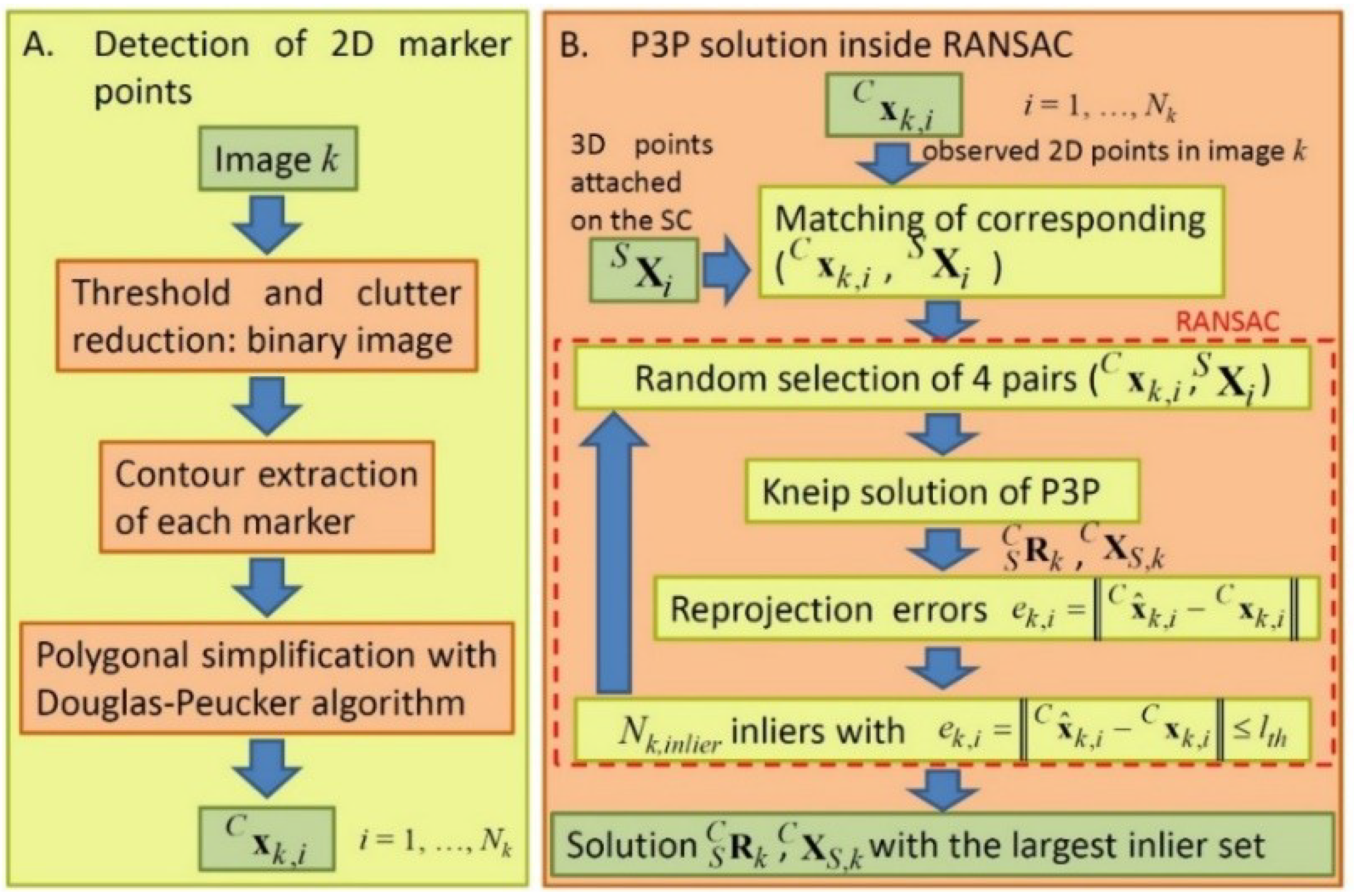
2.1. Step A: Detection of the 2D Marker Points

The pose measurement is based on the 2D position determination of the known 3D points projected in the image plane. The 3D points that are employed come from fiducial markers attached to the external surface of a satellite (a laboratory mock-up as described in Section 4). They are fixed and their positions ${}^{S}X{}_i$ are known in a satellite frame S. In the literature, several different types of fiducial markers are described, e.g., the ARToolKit [22] and Reference [23]. These known types proved to be reliable in many situations and, particularly, in the simultaneous presence of several markers. However, on a spacecraft, there are only a few regular and free surfaces that can accept fiducial markers, as highlighted also by Reference [5]. Thus, the number of employable markers is low. In References [5,6], the selected markers are concentric circles, but the projection of circles on the image plane may yield measurement errors of the detected centroids—as explained in Reference [24]—if the circle size is not small. For these reasons, a simplified set of square markers is designed. Each square marker provides five 3D points ${}^{S}X{}_i$: the four internal vertices and their centroid. The total number of 3D points N_points is the maximum number of 2D projections that can be detected in the acquired images.

Each marker comprises of a known number of internal dots, which are exploited to identify each observed marker. In the images analyzed, the number of internal dots is always correctly detected. In a future improvement, to cope with more severe testing conditions that could cause erroneous detections of the internal dots, the known 3D geometrical constraints among the markers could be employed to perform a consistency check after the marker projections are identified in each image or to enforce detection rules in the images; in the current implementation, the 3D geometrical constraints are employed only for the identification of the vertices of each marker, as described at the beginning of Section 2.2. In the proposed algorithm, possible erroneous matching between the markers in the images and in the 3D space can be identified and eliminated by the RANSAC approach illustrated in Section 2.2.

Another future improvement that could be useful in case of erroneous detection of internal dots is a tracking method for the markers: if the algorithm knows the position of each marker in a previous time instant and a suitable motion model is devised, the position of each marker can be foreseen, providing a support helpful for both position detection and identification of the markers. As explained in the introduction, the exploitation of tracking and previous knowledge is beyond the main purpose of this work.

A camera, mounted on the chaser spacecraft, is aimed to observe the 3D marker points on the target spacecraft. Before the camera can be used for measurements, it should be calibrated; for this purpose, the approach presented in Reference [25] is used. After camera calibration, the measurement procedure begins with the detection of their 2D projections on each acquired image. The detection of markers and their 2D points in each image is described in Figure 2 and an output example is illustrated in Figure 3a. The detection of 2D points comprises the following steps:

• the image binarization using a selected threshold and removal of all small connected regions having less than a set number of pixels; the selected number of pixels is 4, and it depends on the maximum distance of the observed markers and the noise level of the images. This removal reduces the image clutter and the effect of noise, but could make the internal dot detection less reliable.
• the extraction of the internal contour of each square marker, using the Moore-Neighbor algorithm described in Reference [26]; for each detected boundary its perimeter and the number of internal boundaries can be evaluated; only the objects having a number of internal boundaries lower than the maximum number of internal dots and having dimensions compatible with the markers are analyzed. In this way, each observed marker can be identified.
• polygonal simplification using the Douglas–Peucker algorithm, which is called “the most widely used high-quality curve simplification algorithm” in Reference [27]. Each contour extracted in the previous step is a closed polygon with several vertices and the Douglas–Peucker algorithm reduces it to a four-vertices polygon, allowing us to detect the four internal vertices of each square fiducial marker. Then, from the four vertices, the marker centroid is calculated.

In this way, five 2D points ${}^{C}x{}_i$ are detected for each marker in each image and are expressed in the camera frame of reference C. The number of internal dots of each marker allows us to identify which fiducial marker is observed.

2.2. Step B: P3P Solution inside RANSAC

Up to now, the algorithm knows five 2D projections for each identified marker and which marker they belong to, but does not know the order of the observed vertices. Before any pose evaluation can be performed, the algorithm has to associate each detected 2D vertex in the camera frame C with the corresponding 3D point in the satellite frame S. The 3D geometrical constraints among the markers and their known shape are employed to enforce rules on the detected vertices, in terms of lines and distances in the acquired images. For instance, with reference to Figure 3b, the two top vertices v_1,1 and v_1,4 of the marker with one internal dot (marker 1) will always be roughly aligned with the two top vertices v_4,1 and v_4,4 of marker 4 (with four internal dots) and vertex v_1,1 will always have a distance from the aligned vertices v_4,1 and v_4,4 larger than vertex v_1,4. The same two rules (alignment and distance) are verified by the vertices v_1,2, v_1,3, v_4,2, v_4,3. Thus, suppose we want to identify the vertices of marker 1 (detected as described in Section 2.1):

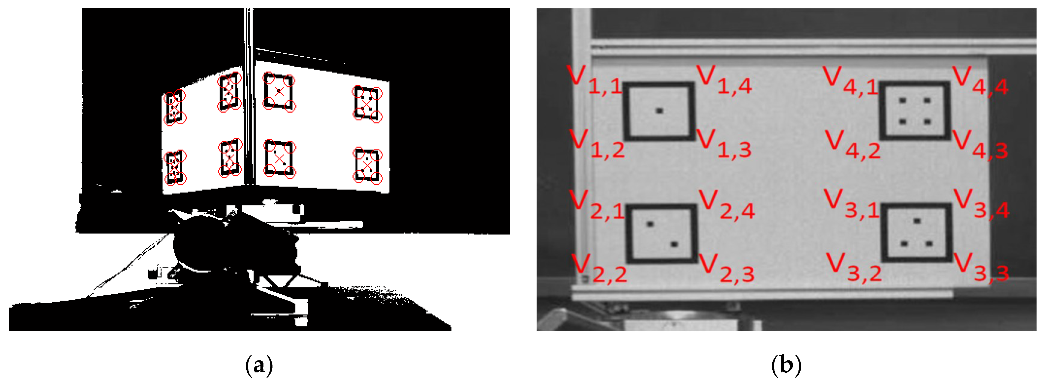
• two adjacent vertices v_1,x and v_1,y are considered;
• the algorithm verifies if they are aligned with two vertices of marker 4 or marker 2; suppose they are aligned with two vertices of marker 4;
• the algorithm evaluates which one is farther from the vertices of mark 4; suppose v_1,x is farther; it means v_1,x could be v_1,1 or v_1,2, while v_1,y could be v_1,3 or v_1,4;
• the other vertex v_1,z adjacent to v_1,x is considered;
• the algorithm evaluates if v_1,x or v_1,z is nearer to the vertices of marker 2; suppose v_1,x is nearer;
• in this case v_1,x = v_1,2, v_1,y = v_1,3, v_1,z = v_1,1, and the fourth vertex of marker 1 remains identified.

Different orders and associations are obtained if the verifications at points 2, 3, 5 yield different results. Similar rules on the image plane allow us to perform the correct matching between the detected vertices of all the markers in the projected images and in the 3D space.

In this way, for each 2D observed point ${}^{C}x{}_i$ a corresponding 3D point ${}^{C}X{}_i$ is associated in the spacecraft frame S. An image is acquired in every camera-target relative pose; each observed 2D point depends on the corresponding 3D point and on the camera-target relative pose; thus, for each image k (k = 1, …, N_poses), the matching phase yields N_k pairs (${}^{C}x{}_{k,i}$, ${}^{S}X{}_i$) with i = 1, …, N_k ≤ N_points.

After the pairs (${}^{C}x{}_{k,i}$, ${}^{S}X{}_i$) are evaluated, a first approximation of the relative pose can be obtained using one of the solutions of the PnP problem cited in the introduction. Preliminary tests were performed using three different approaches: Gao [14], EPnP [9], and Kneip [16]. The results, reported in Section 5, highlight the advantage of the Kneip solution [16], which is selected for the second step B. The Kneip method is chosen also because it is direct (the intermediate step of calculating the 3D points ${}^{C}X{}_i$ in the camera frame C is completely eliminated), closed-form (no iterations are needed), and requires only three plus one pairs. Using three pairs (${}^{C}x{}_{k,i}$, ${}^{S}X{}_i$), four rotation matrices ${}_S{}^{C}R{}_j$ from the satellite frame S to the camera frame C and four position vectors ${}^{C}X{}_{S,j}$ of the satellite frame S expressed in the camera frame C, with j = 1, …, 4, can be evaluated. The four rotation matrices ${}_S{}^{C}R{}_j$ and position vectors ${}^{C}X{}_{S,j}$ are evaluated from the roots of a fourth order polynomial, which is solved by applying Ferrari’s closed form solution. The equations are described in four pages of Reference [16], and the software implementation of the computation procedure is available in an on-line directory reported in Reference [16]. Then, the 3D point ${}^{S}X{}_i$ of a fourth pair (${}^{C}x{}_{k,i}$, ${}^{S}X{}_i$) is re-projected in the image k using the four roto-translations evaluated ${}_S{}^{C}R{}_j$, ${}^{C}X{}_{S,j}$ and the solution which provides the smallest re-projection error is selected as the correct rotation matrix ${}_S{}^{C}R{}_k$ and translation ${}^{C}X{}_{S,k}$. The re-projection equations can be found in Reference [8].

Due to the small number of points required and to the closed-form, the Kneip solution [16] of the P3P problem is particularly efficient and suitable to be embedded in a RANSAC scheme, [28]. For each image k, the Kneip method is applied several times and, in each iteration, the following steps are performed, see Figure 2: four pairs (${}^{C}x{}_{k,i}$, ${}^{S}X{}_i$) are randomly selected; the rotation ${}_S{}^{C}R{}_k$ and translation ${}^{C}X{}_{S,k}$ are evaluated with Kneip; the 2D re-projections ${}^C\widehat{x}{}_{k,i}$ of all the available 3D points ${}^{S}X{}_i$ are calculated; the N_k,inlier (with N_k,inlier ≤ N_k ≤ N_points) pairs whose re-projection error $e_{k,i}=\Vert {}^C\widehat{x}{}_{k,i}-{}^{C}x{}_{k,i}\Vert$ is less than a threshold lth are considered inliers and define a consensus set of the examined iteration. At the end of the RANSAC scheme, the set with the larger consensus (e.g., the maximum number of inliers) is selected. Even if the application of the RANSAC scheme in presence of observed fiducial markers with known shapes may appear unnecessary, the experimental tests highlight that it is useful to reject inaccurate 2D points detected in images. Inaccurate 2D positions can happen mainly due to a partial visibility or high deformation of an observed marker. The outputs of the RANSAC procedure are two: the selected roto-translation ${}_S{}^{C}R{}_k$ and ${}^{C}X{}_{S,k}$ for each image k, calculated by the Kneip solution, and the set of pairs (${}^{C}x{}_{k,i}$, ${}^{S}X{}_i$), with i = 1, …, N_k,inlier ≤ N_k ≤ N_points, which are considered inliers.

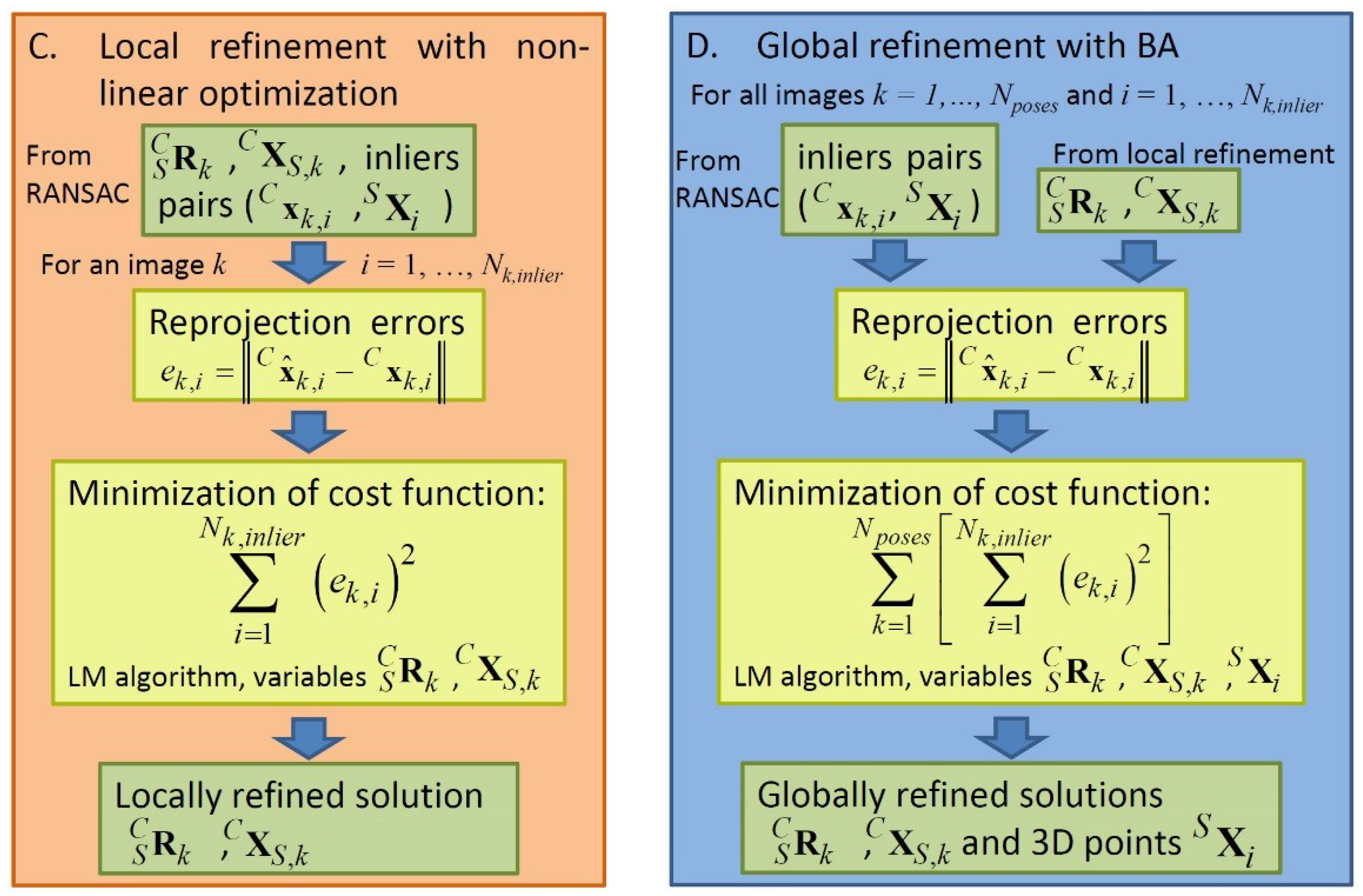
2.3. Step C: Local Refinement with Non-Linear Optimization

For each relative position and orientation between the camera (chaser) and the spacecraft (target), i.e., each image k, the rotation matrix ${}_S{}^{C}R{}_k$ and the translation vector ${}^{C}X{}_{S,k}$ found by the P3P solution plus RANSAC, can be refined using a non-linear optimization. The scheme is illustrated in Figure 4 (left). The rotation has to be expressed by three Euler angles or a quaternion. In this work, the Euler angle approach is selected since it gives us a clear understanding of the obtained results.

For each image k, if the roto-translation ${}_S{}^{C}R{}_k$ and ${}^{C}X{}_{S,k}$ between the camera and the satellite is known, it can be used to re-project the 3D points ${}^{S}X{}_i$ of all the N_k,inlier pairs (${}^{C}x{}_{k,i}$, ${}^{S}X{}_i$) on the image k, obtaining the reprojections ${}^C\widehat{x}{}_{k,i}$. Then, the 2D reprojection errors can be evaluated and the following cost function can be calculated:

$${\displaystyle \sum _{i=1}^{N_{k,inlier}}{\left(e_{k,i}\right)}^2=}{\displaystyle \sum _{i=1}^{N_{k,inlier}}{\Vert {}^C\widehat{x}{}_{k,i}-{}^{C}x{}_{k,i}\Vert }^2}$$

(1)

In Equation (1) only the N_k,inlier pairs coming from the RANSAC procedure are used. The Equation (1) becomes the cost function of a minimization problem with variables ${}_S{}^{C}R{}_k$ and ${}^{C}X{}_{S,k}$. A numerical solution of the minimization problem can be found with the Levenberg–Marquardt (LM) algorithm [29]. The LM algorithm requires the initial values of the variables ${}_S{}^{C}R{}_k$ and ${}^{C}X{}_{S,k}$ to start the minimum search. In this case, the values obtained at the end of the previous step B are employed. During the searching process, the N_k,inlier pairs (${}^{C}x{}_{k,i}$, ${}^{S}X{}_i$) with i = 1, …, N_k,inlier are kept constant, while the variables ${}_S{}^{C}R{}_k$ and ${}^{C}X{}_{S,k}$ are iteratively changed. At the end of the searching process, the LM algorithm provides the refined roto-translation ${}_S{}^{C}R{}_k$ and ${}^{C}X{}_{S,k}$. As illustrated in Figure 1, the steps A–C are repeated for all the N_poses camera-satellite relative poses. The local refinement step C involves only the N_k,inlier pairs (${}^{C}x{}_{k,i}$, ${}^{S}X{}_i$) of the considered image k and the associated relative pose.

2.4. Step D: Global Refinement with BA

The measurement phase described in the previous Section 2.3 is called local refinement since the optimization is performed for each relative position and orientation and affects only the evaluated roto-translation. Up to the local refinement phase, the 3D point positions ${}^{S}X{}_i$ in the spacecraft frame S and their uncertainties are obtained by a manual and direct measurement with a caliper and define an initial 3D map. Since these 3D point positions are the input quantities of the examined measurement procedure and they are kept constant up to the local refinement phase, the errors in their measurements can yield systematic effects on the final indirect measurement of the relative roto-translation. The following Section 5 of the experimental results will show that the analysis described in the previous work [8] is partially affected by a systematic effect due to the 3D point positions (3D initial map). To compensate for this undesired systematic effect, in the present work, a BA global refinement is introduced.

After the roto-translations ${}_S{}^{C}R{}_k$ and ${}^{C}X{}_{S,k}$ for all the considered relative positions and orientations (k = 1, …, N_poses) are locally refined as described in Section 2.3, the BA approach—References [30,31]—adjusts all the already-evaluated roto-translations and the 3D point positions, i.e., the 3D map, to globally minimize the sum of the squared re-projection errors. With reference to Figure 4 (right), the input quantities of this step D are all the roto-translations ${}_S{}^{C}R{}_k$ and ${}^{C}X{}_{S,k}$ with k = 1, …, N_poses, which come from the iterated local refinement step C and all the pairs (${}^{C}x{}_{k,i}$, ${}^{S}X{}_i$) of inliers with k = 1, …, N_poses and i = 1, …, N_k,inlier, which are identified by the RANSAC scheme repeated for all relative poses N_poses.

Similarly to the local refinement step C, a new cost function can be defined:

$${\displaystyle \sum _{k=1}^{N_{poses}}\left[{\displaystyle \sum _{i=1}^{N_{k,inlier}}{\left(e_{k,i}\right)}^2}\right]}={\displaystyle \sum _{k=1}^{N_{poses}}\left[{\displaystyle \sum _{i=1}^{N_{k,inlier}}{\Vert {}^C\widehat{x}{}_{k,i}-{}^{C}x{}_{k,i}\Vert }^2}\right]}$$

(2)

In this case, the constants that do not change during the minimum searching process are all the detected 2D points ${}^{C}x{}_{k,i}$ that belong to a pair of inliers (${}^{C}x{}_{k,i}$, ${}^{S}X{}_i$), with k = 1, …, N_poses and i = 1, …, N_k,inlier ≤ N_k ≤ N_points, while the variables that are changed in the searching process are all the roto-translations ${}_S{}^{C}R{}_k$ and ${}^{C}X{}_{S,k}$ with k = 1, …, N_poses and all the 3D points ${}^{S}X{}_i$ with i = 1, …, N_points. The LM, which is used also for the minimization of the cost function (Equation (2)), starts the minimum search from the values of ${}_S{}^{C}R{}_k$ and ${}^{C}X{}_{S,k}$ obtained at the end of the iterations of the previous step C, and from the values of ${}^{S}X{}_i$ that come from the manual direct measurements.

The BA approach yields both refined roto-translations and a refined set of 3D points. In the present work, two different implementations of BA are considered and compared. In the first implementation, the final output quantities are the roto-translations ${}_S{}^{C}R{}_k$ and ${}^{C}X{}_{S,k}$ with k = 1, …, N_poses obtained at the end of the BA approach as described. In this case, the globally refined 3D positions ${}^{S}X{}_i$, obtained as additional output of the BA approach, are not used.

In a second implementation (see Figure 5) the whole procedure as described and comprising steps A–D is applied to a subset of the available N_poses relative poses, and then only the steps A (the 2D point detection), B (the P3P solution inside RANSAC) and C (the local refinement with non-linear optimization) are performed for all the N_poses relative poses, using as 3D points ${}^{S}X{}_i$ those refined by the BA approach. In this case, the roto-translations obtained at the end of the BA approach are not considered, while the globally refined 3D points ${}^{S}X{}_i$ with i = 1, …, N_points and all the images k with k = 1, …, N_poses become the input of the simplified procedure with steps A–C. Obviously, for those images whose 2D points ${}^{C}x{}_{k,i}$ were already detected for the whole procedure A–D, the first step A is not repeated, but the same 2D points ${}^{C}x{}_{k,i}$ are employed. With reference to Figure 5, in the second implementation, the whole procedure is applied with a number of poses N′_poses ≤ N_poses and the only outputs that are retained are the globally refined 3D points ${}^{S}X{}_i$ (bottom of Figure 5). Then the steps A–C inside the second red rectangle of Figure 5 are repeated for all the poses N_poses, using the new refined 3D points (in the green input rectangle). The following Section 5 will compare the results of these two implementations.

3. Uncertainty Evaluation

The uncertainties of the relative positions and orientations between the target spacecraft and the camera (chaser) are evaluated using the procedures foreseen by References [32,33] in case of an indirect measurement with a plurality of input quantities. As explained in Reference [8], the Monte Carlo (MC) propagation approach is chosen due to the non-linearity of the measurement method. The MC method allows us to propagate the uncertainties evaluated for the input quantities to the uncertainties of the output relative pose. According to the MC method, the uncertainty propagation is performed by a numerical procedure, which allows us to take into account the non-linearity of the functional relationship between the inputs and outputs. The Kline–McClintock propagation formula is not used since it approximates (linearization) the propagation model.

The input quantities are the intrinsic parameters of the camera, the 3D point positions in the satellite frame S, the positions of the 2D points detected on each image. The uncertainties of the intrinsic parameters of the camera are evaluated using the Zhang procedure [25] for camera calibration, while the uncertainty of each 3D point is evaluated from repeated experimental measurements manually acquired by three different operators using a caliper, according to the type A contributions described in Reference [32]. For the 2D positions in each image, three uncertainty contributions are considered, evaluated and then combined together: the effect of the selected threshold for image binarization, the inexact detection of the four internal vertices of each marker, and the residual uncorrected optical distortions. The contribution of the threshold selection is evaluated by changing the threshold level within a suitable range. The contribution of the contour extraction algorithm and the Douglas–Peucker polygonal simplification is evaluated experimentally comparing the vertices detected by the algorithm and manually by an operator in different orientations of the spacecraft. Finally, the contribution of the optical distortions that the distortion model is not able to remove is evaluated acquiring a planar chessboard orthogonal to the optical axis.

The uncertainties of the 2D points are evaluated more carefully than in Reference [8], experimentally taking into account that the Douglas–Peucker algorithm can sometimes yield a 2D point near but not exactly coincident with the desired corner of a marker. For this reason, the evaluated uncertainties depicted in Section 6 and Section 7 may be slightly larger than those obtained in Reference [8] using the same non-linear approach without BA.

The uncertainties evaluated for the output relative roto-translations allow us to verify the compatibility of the experimentally obtained errors (the difference between the values obtained by the vision system and those obtained by the reference instrumentation).

4. Experimental Set-Up

The purpose of the experimental tests is to calibrate the whole measurement system for the satellite position and orientation measurement. To this aim, a satellite mock-up, provided with eight square fiducial markers as depicted in Figure 6, is mounted on a high precision motor-driven rotary stage and on a linear slide, which allows us to impose linear displacements and/or rotations to the satellite mock-up, while the camera is fixed. At the same time, the rotary stage and linear slide can measure the roto-translations and are used as reference instruments to evaluate the measurement errors.

The set-up, comprising of the rotary stage, the linear slide, and the camera, is the same as that employed and described in Reference [8], which can be consulted for details. Twenty-two different positions along the linear slide are tested, with a longitudinal step of 50 mm. The smallest distance camera—mock-up is 1500 mm, while the farthest one is 2550 mm. For each linear position, the mock-up attitude is varied within 90° in 2° steps (when the attitude angle is near 0° and 90°, the observed markers are substantially orthogonal to the optical axis, with an evaluated misalignment of 1.3°). Thus, a total number of 22 × 45 = 990 measurements of position and orientation are acquired using the fixed camera and are compared with the corresponding imposed values. The experimental data set, i.e., the imposed rotations and translations and the corresponding acquired images are the same employed in Reference [8]. Thus, the error results illustrated in Section 5, Section 6 and Section 7 can be directly compared with Reference [8], while the obtained uncertainties may be slightly larger than in Reference [8], as explained in Section 3. Figure 7 shows the images acquired by the camera when the distance between the camera and the satellite reaches its maximum (a,b,c) and minimum (d,e,f) value, and when the rotation angle is 0° (a,d), 45° (b,e), 90° (c,f). The partial occlusion of the markers, which happens when the mock-up is near its minimum distance, affects the number of observed 2D points.

The algorithm, described in Section 2, measures all three Euler angles and three relative position components, but the experimental set-up allows us to evaluate the errors only for two degrees of freedom: one translation and one rotation. The rotary stage allows us to impose and directly measure only the first Euler angle which is a rotation around a vertical axis and the position along the linear slide whose longitudinal axis has an evaluated misalignment of 1.3° with reference to the optical axis of the camera. Thus, the angular error can be assessed only around the vertical axis. Similarly, from the three position components measured by the described approach, the total distance between the camera frame C and the spacecraft frame S is evaluated and it is compared with the imposed position along the linear slide, defining the position error depicted in the following figures. The accuracy of the linear slide (≤1 mm) and the rotary stage (≤72 arcsec) is much better than the uncertainties achievable by the proposed method; thus, they are employed as reference instruments and their uncertainties are neglected.

In the employed laboratory set-up, the images of the markers are acquired in normal/good lighting conditions, while in a typical space application, the acquired scene could be affected by a low light condition and presence of extremely bright areas and deep shadows. These space lighting conditions could worsen the uncertainties of some detected 2D points and, consequently, of the final results. The harsh lighting conditions of the space environment are certainly an additional uncertainty source and should be considered in a future work; the possible aid of a marker illumination system may also be analyzed. However, an additional uncertainty source could also hide or mask the possible correlations between the pose errors/uncertainties and the geometrical distribution and position of the markers, making the correlations less clear to be observed.

That said, the increase of the 2D point uncertainty due to poor lighting can make the re-projection error larger than the threshold lth of the RANSAC procedure. Thus, the net effect is a reduction of the available pairs (${}^{C}x{}_{k,i}$, ${}^{S}X{}_i$) of inliers, which generally has a negative effect on the obtained errors and uncertainties. This is confirmed by our results as described in Section 7. However, as it will be shown in Figure 24, it is worth pointing out that a reduction of the number of points (from a maximum value of 38 to a flat value of 14 in Figure 24) could be associated only with a slight worsening of the final error.

The results that will be described in Section 5, Section 6 and Section 7 are obtained implementing the numerical measurement procedure on a desktop PC using Matlab^®. Since neither the hardware nor the software code is optimized for a real-time application on a satellite, the proposed analysis cannot give useful indications about the absolute speed and timing of the procedure. However, as it will be explained in the following Section 5, the selected implementation of the BA approach may not increase the computational burden during the real-time measurements.

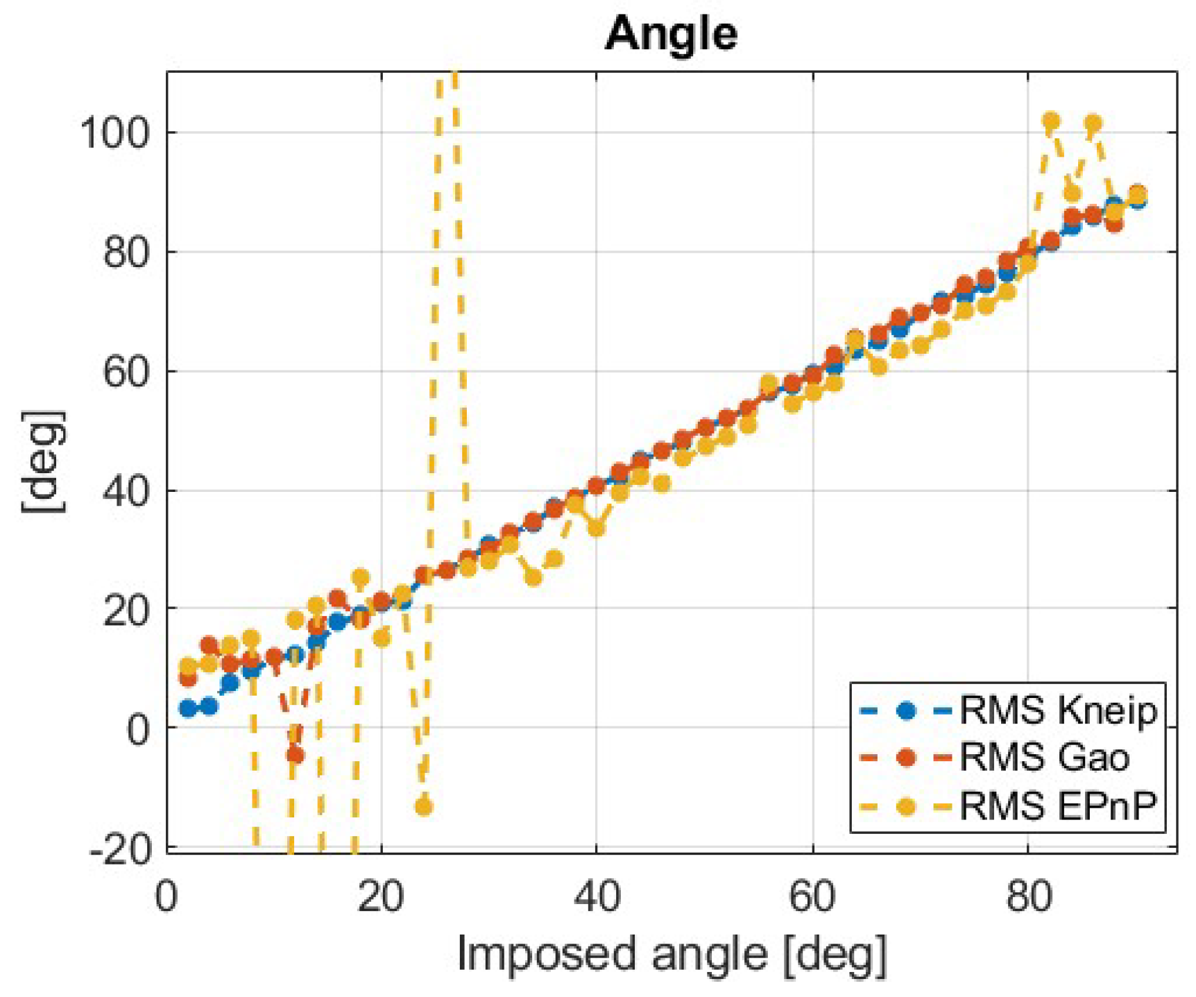
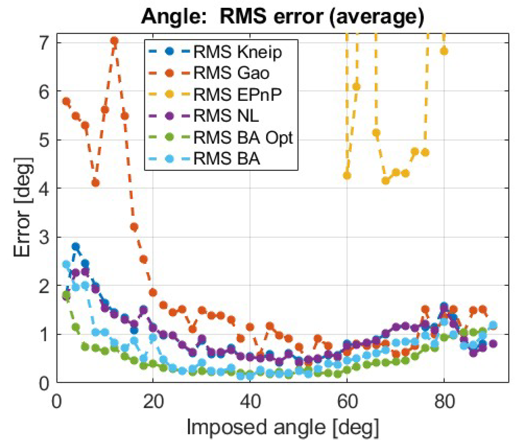
5. Results: Preliminary Method Comparison

In a preliminary phase of the presented work, three different solutions of the general PnP problem were analyzed and compared: Gao [14], EPnP [9], and Kneip [16]. For the two additional methods (Gao and EPnP) the implemented code can be found from the internet: the Gao solution is comprised in the Computer Vision Toolbox of Matlab, while the EPnP implementation can be downloaded from a web link reported in Reference [9]. For the three methods, Figure 8 compares the evaluated attitude angle in a single position, while Figure 9 shows the root mean square (RMS) errors calculated for each angle considering all the 22 positions. In our application, the number of available pairs (${}^{C}x{}_{k,i}$, ${}^{S}X{}_i$) is rather low (as it will be depicted in Figure 22, it varies from 14–16 to 38) and the EPnP solution had problems with some internal singular matrices evaluated during the calculation. The best errors are obtained by the Kneip solution which is selected for the step B of the measurement procedure.

As described in Section 2.4 in the preliminary comparison of methods, two different implementations of the BA approach are compared: the first implementation executes the four steps A–D as described for all the available relative poses N_poses, while the second one executes the four steps A–D on a sub-set of N′_poses (≤N_poses) poses, and then repeats the steps A–C (without the BA approach) for all the relative poses N_poses, using the refined 3D points obtained by BA; see Figure 5.

In this second case, the steps A–D are executed with the main purpose of evaluating a globally refined set of 3D points. A clear advantage of the second implementation is that the relative pose is evaluated using only the steps A–C, while the BA approach (with its additional computational burden) can be executed only once, e.g., before the real-time measurement begins, or only when it is needed, e.g., when the thermal deformations may have slightly changed the positions of the 3D points.

An important aspect is the choice of the relative poses used to apply the BA refinement of the 3D points. In this work, eight linear positions and eight angular rotations (a total number of 8 × 8 = 64 = N′_poses ≤ N_poses = 990) were selected to cover the whole linear and angular measurement range.

Figure 9, together with the three PnP solutions, also shows the RMS attitude error versus the imposed rotation obtained:

• after the steps A–C, i.e., after the local refinement with the non-linear minimization (purple line);
• after the steps A–D, i.e., after the global refinement with the BA approach according to the first implementation (light blue line); in this case, the BA approach is applied considering all the available relative poses N_poses.
• According to the second implementation of the BA approach (green line).

The result is that the second implementation yields the lowest error. Due to the implementation advantage (only the steps A–C can be implemented in real-time) and this preliminary result, the second implementation of the BA approach is selected and is employed in all the analyses presented in Section 6 and Section 7. Using the second implementation, the benefits of the BA approach that will be presented in the following Section 6 can be obtained without any increase of the computational burden or worsening of the speed and timing performance of the algorithm during the real-time measurements. The reason is that the global refinement of the 3D points (steps A–D) can be embedded into a calibration phase and can be performed only at the beginning of the operational activities of the system or on request when it is deemed useful. After the images of the markers are acquired, this calibration phase with BA can be performed “off-line” using the on-board hardware resources without any timing constraints or even on the ground (if the images are available), since the purpose is the refinement of the 3D points and not the relative pose evaluation.

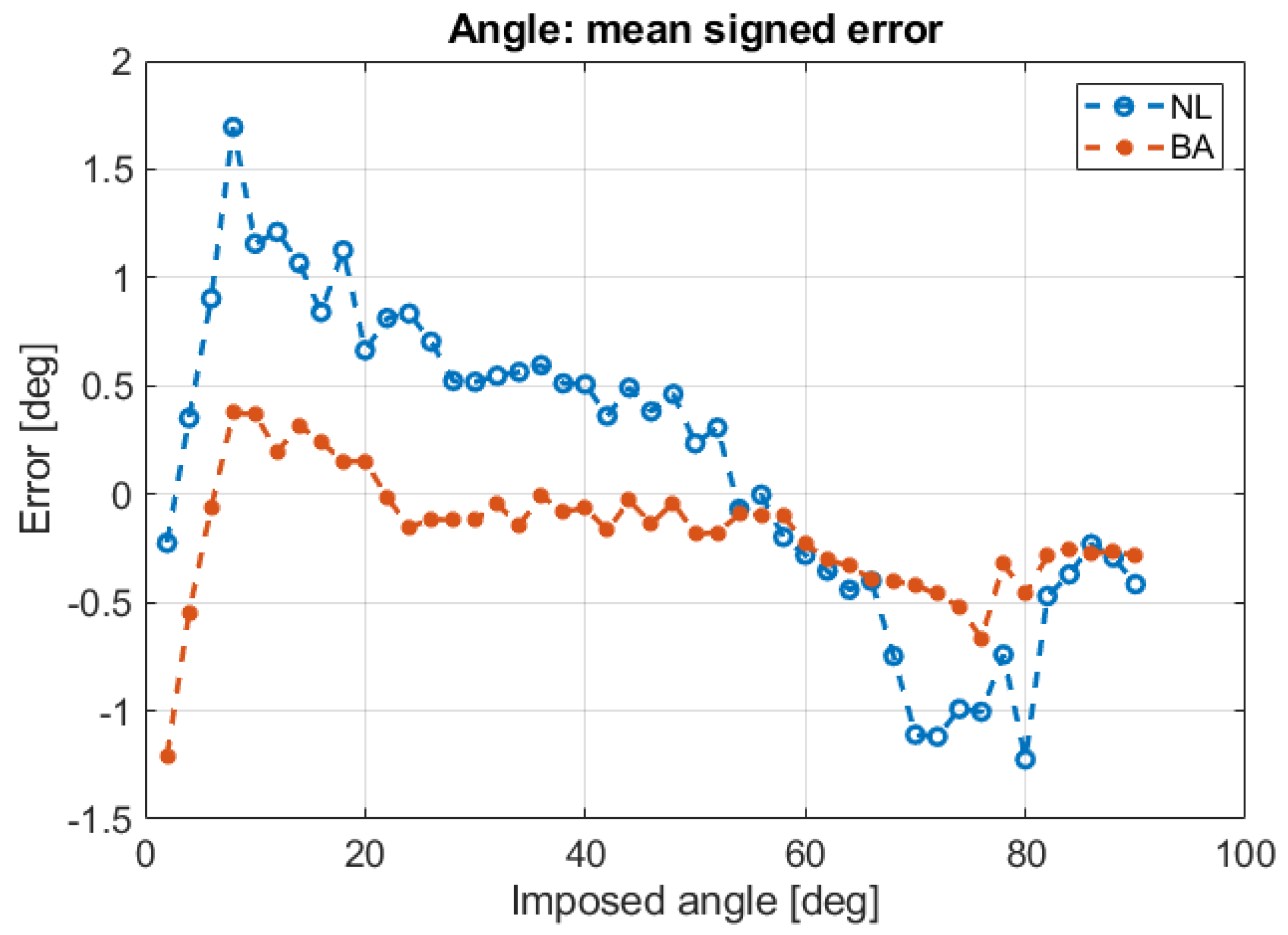
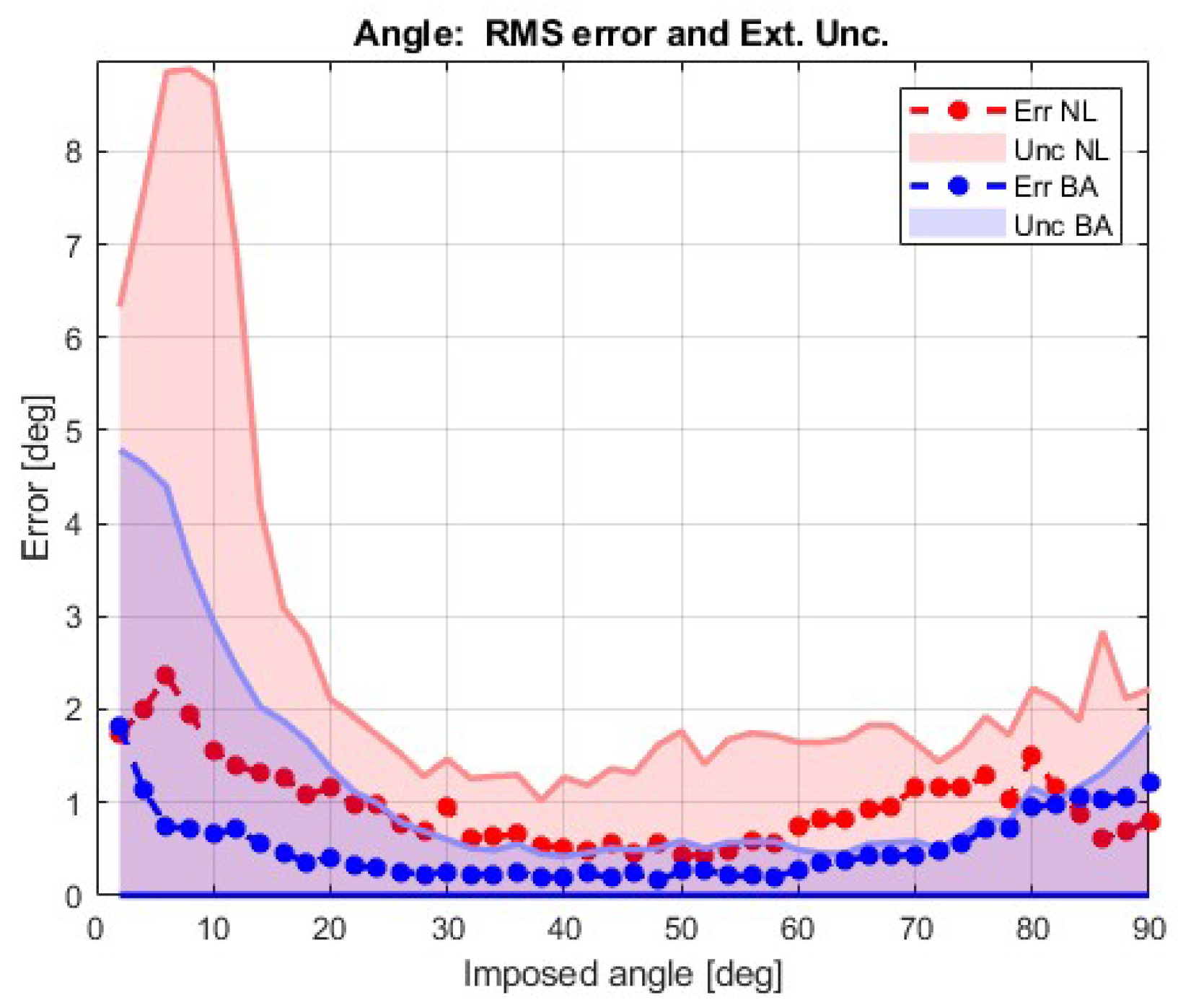
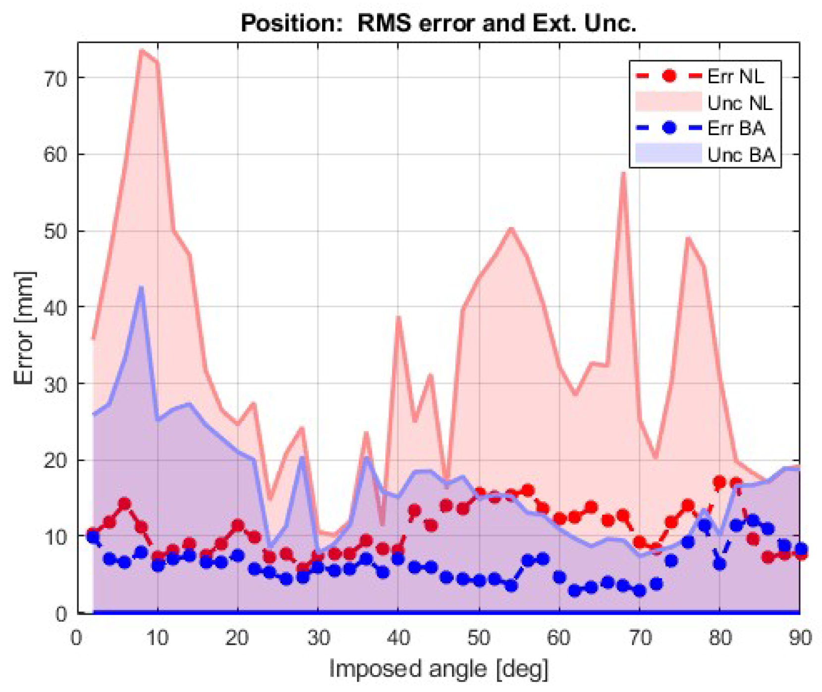
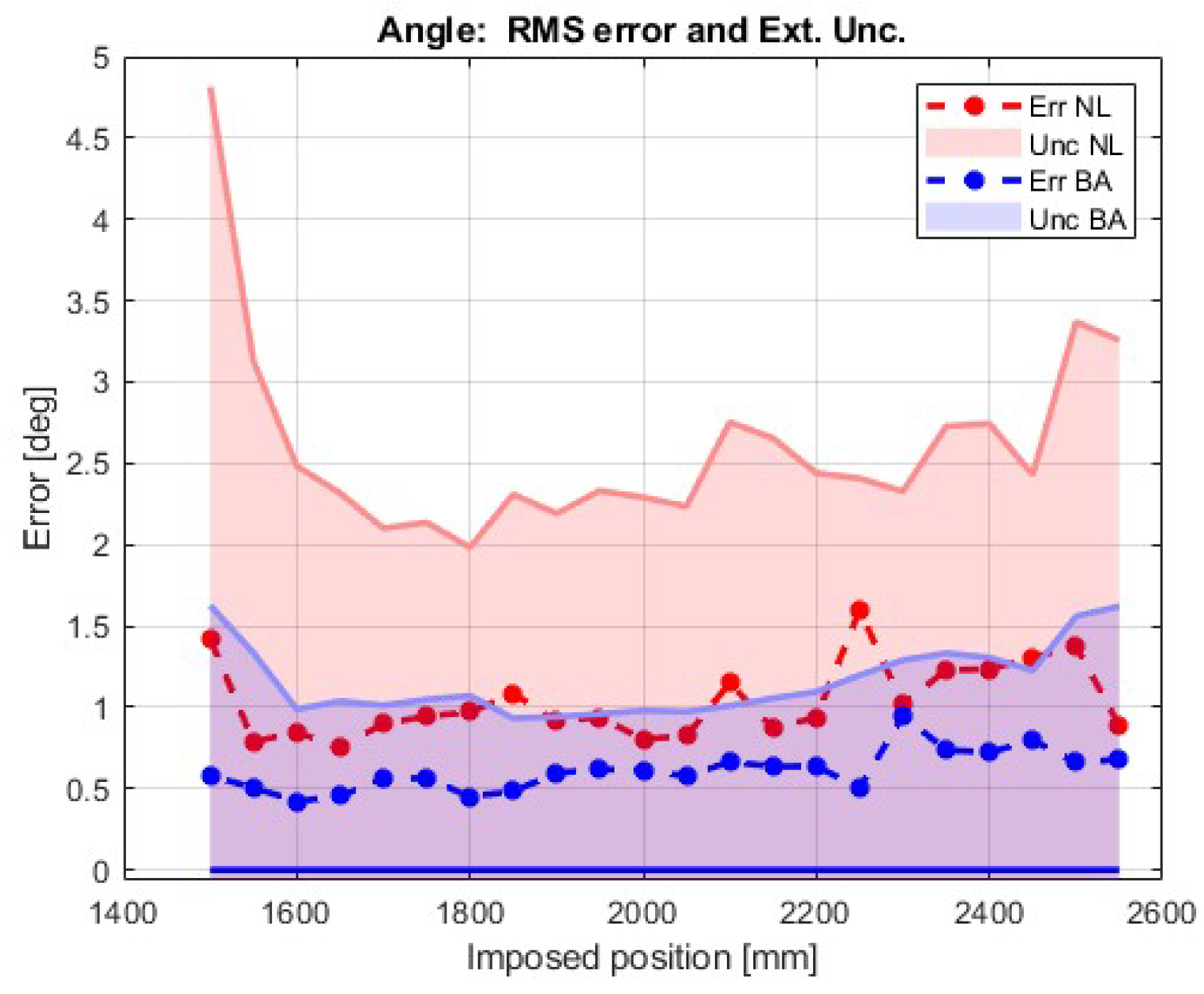
6. Results: Effect of the Bundle Adjustment (BA)

A more in-depth analysis of the results without the BA approach as in Reference [8], allows us to find out a partial systematic effect due to the measurements of the 3D points. In detail, Figure 10 (blue line) shows the angular errors obtained without the BA approach, averaged for the 22 distances versus the rotation angle. These values cannot be directly compared with the errors depicted in the following Figure 11, Figure 12, Figure 13 and Figure 14, since they are the average of positive and negative values, while in Figure 11, Figure 12, Figure 13 and Figure 14, an RMS calculation is carried out. The blue line in Figure 10 clearly shows that there is an average angular overestimation for angles lower than ~50° and vice versa for larger angles. This systematic effect can potentially modify the experimental conclusions. However, the orange line in Figure 10 shows the same averaged errors in the case with the BA approach. It is clear that, after the 3D point positions are refined by BA, the systematic over/under-estimation is heavily reduced, even if the 3D points refined with the BA remain compatible with the position uncertainty of the 3D points measured by the caliper.

After the reduction of the systematic effect, allowed by the BA approach (second implementation), Figure 11 and Figure 13 compare the measurement error (difference between the measured valued and the imposed one) for the rotation around the vertical axis obtained with the non-linear approach as in Reference [8] (red line with circular dots) and with the BA approach (blue line with circular dots). The same figures also depict the evaluated extended uncertainties as shaded areas. Figure 12 and Figure 14 show the measurement errors and the corresponding uncertainties for the linear position without BA (red line and shaded area) and with BA (blue line and shaded area). Figure 11 and Figure 12 illustrate the root mean square (RMS) errors calculated for each angle considering all the 22 positions, while Figure 13 and Figure 14 depict the RMS errors calculated for each position considering all the 45 angles. In a similar way, Figure 11 and Figure 12 show the extended uncertainties with a level of confidence of 99.7% evaluated for each angle, averaging all the 22 positions, while Figure 13 and Figure 14 depict the extended uncertainties evaluated for each position, averaging all the 45 rotations. Figure 11, Figure 12, Figure 13 and Figure 14 show that the observed measurement errors are compatible with the evaluated extended uncertainties and highlight the significant improvement provided by the global refinement due to the BA approach. In several cases, the error or uncertainty obtained with BA is less than half the corresponding value without BA. Thus, considering the achievable errors and uncertainties, a clear result of the presented analysis is the undoubted superiority of the approach with the BA refinement.

As it can be observed in Figure 11, a clear effect highlighted by the experimental tests is a reduction of the angular error and uncertainty when the rotation angle is around 45–50°. This effect was already present in Reference [8], but the interesting result of the present work is that the same behavior is still present even after the systematic effect correction carried out by the BA approach. The possible causes of this reduction of angular error and uncertainty near 45–50° will be discussed in Section 7.2 when the influencing parameters are analyzed.

As in Reference [8], another effect, highlighted by Figure 14 and present after the BA correction of the systematic effect discussed above, is the increase with distance of the position errors and uncertainties. A similar error and uncertainty increase can be observed also for the attitude angle (see Figure 13) even if it is less evident. The reason is that an increase in the distance of the observed object yields smaller observed markers. The performed tests allow us to quantify this effect on the obtained measurements. The same effect of the distance will also be analyzed in Section 7.8.

7. Results: Influencing Parameters

To investigate the possible causes and the most influencing characteristics that affect the error and uncertainty of rotation angle and position, the following eight parameters are defined, with reference to Figure 15:

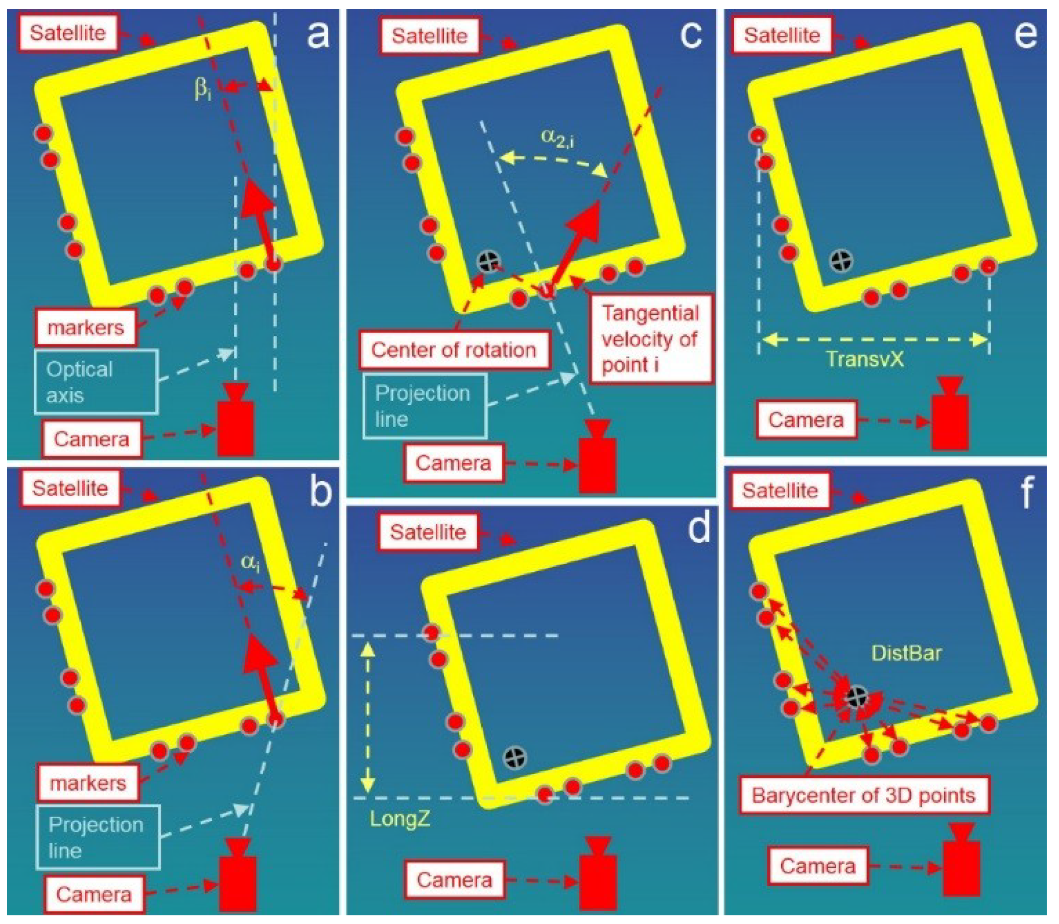
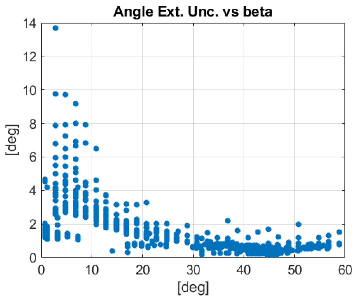
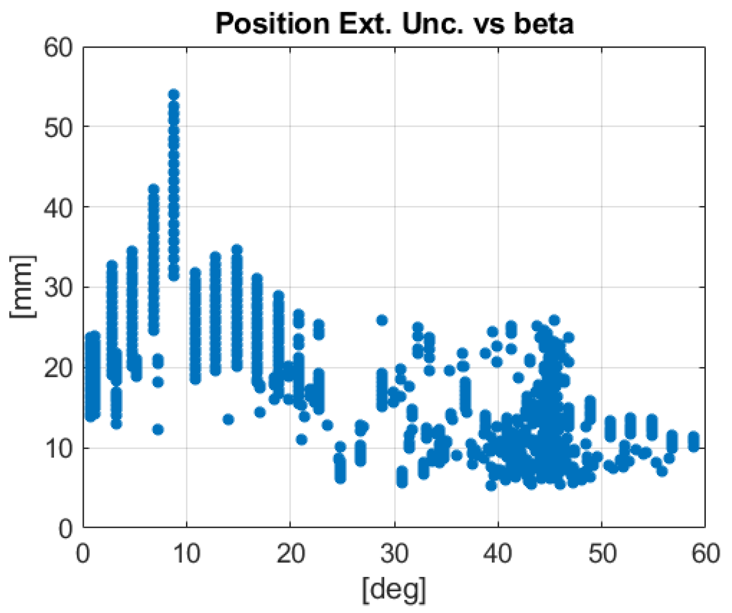
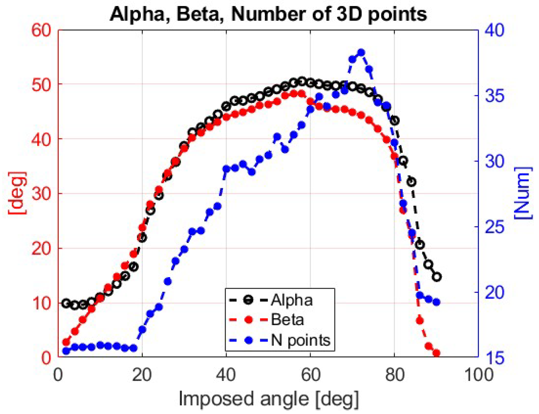
• The mean angle β between the optical axis and the normal to the marker plane of each point that passes the RANSAC selection, see Figure 15a.
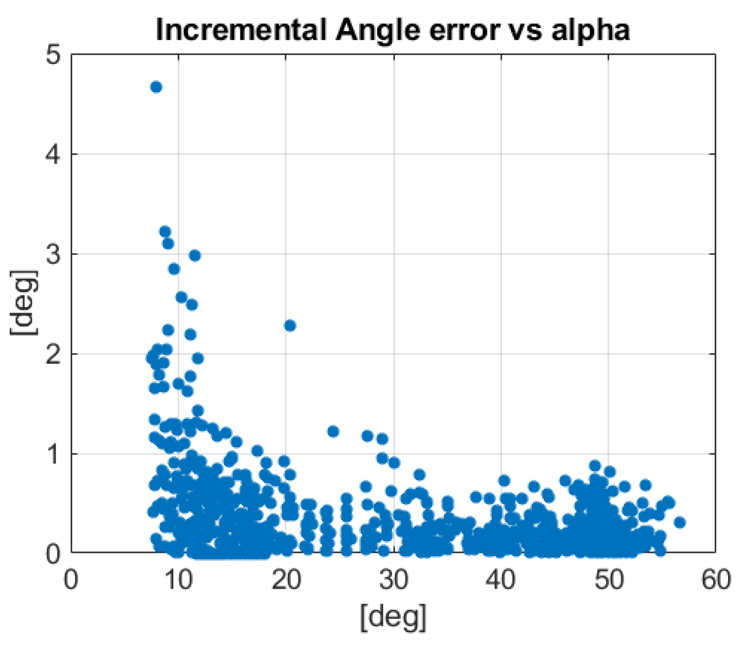
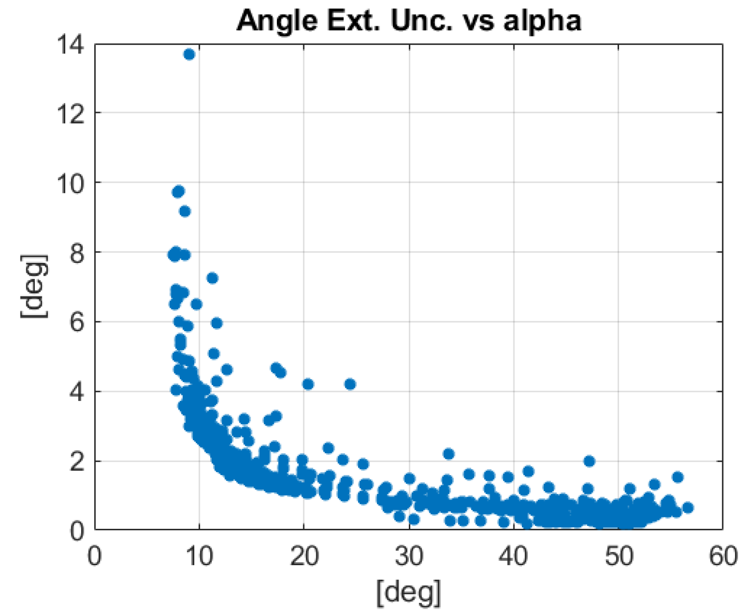
• The mean angle α between the camera projection line and the normal to the marker plane of each point that passes the RANSAC selection, see Figure 15b.
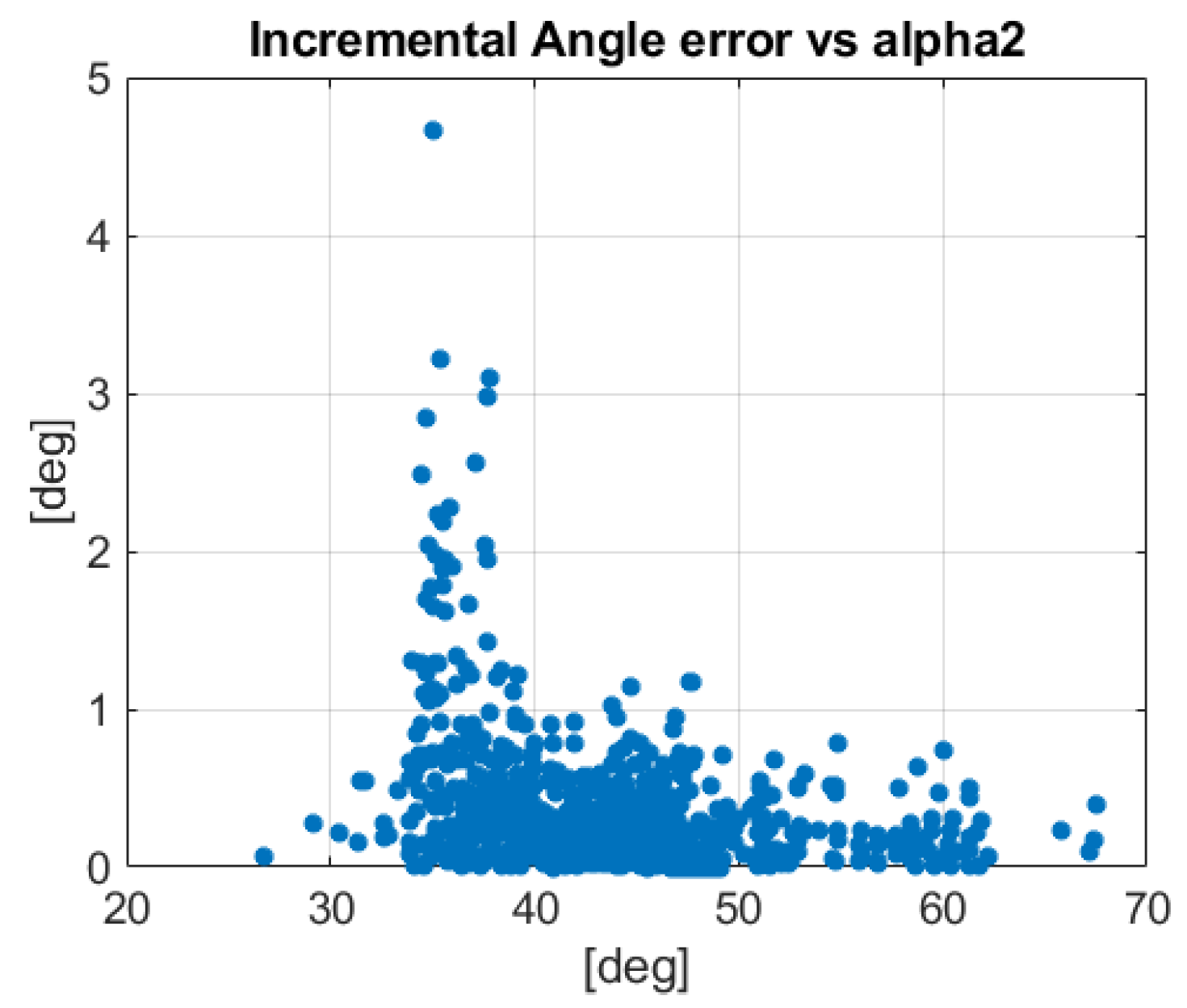
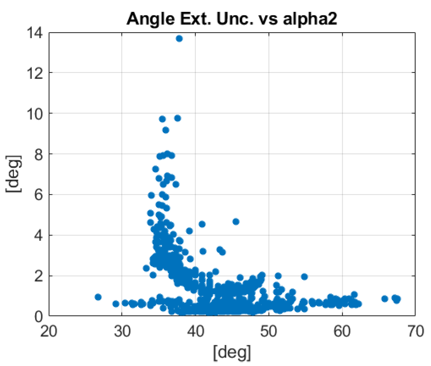
• The mean angle α₂ or α₃ between the tangential or local velocity and the camera projection line of each point that passes the RANSAC selection. When the rotations are examined, the tangential velocity with reference to the rotation center is employed as depicted in Figure 15c, for the calculation of α₂. If the positions are analyzed, the local velocity of the translation motion is considered for each marker. In the linear displacement case, the direction of the local velocity is the same for all the markers and is considered parallel to the longitudinal slide of the set-up for the calculation of the mean angle α₃.
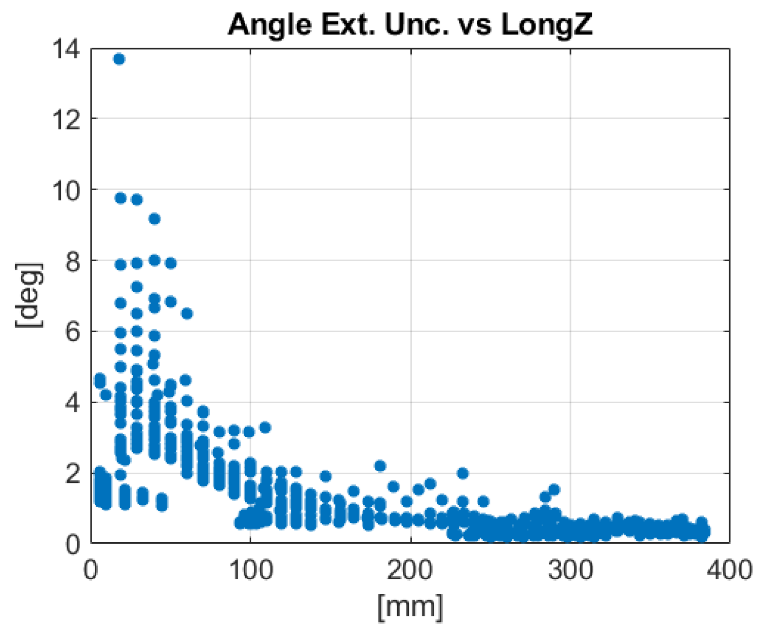
• The maximum longitudinal distance LongZ of the 3D points, see Figure 15d.
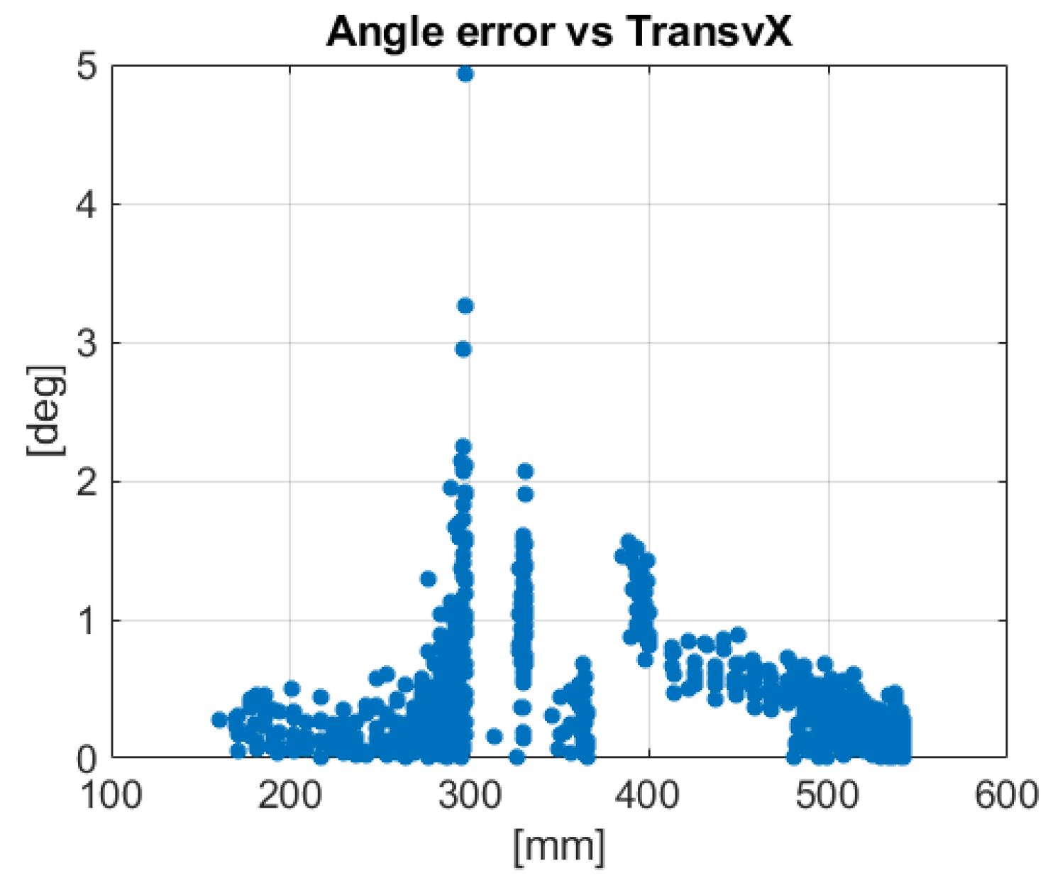
• The maximum transverse distance TransvX of the 3D points, see Figure 15e.
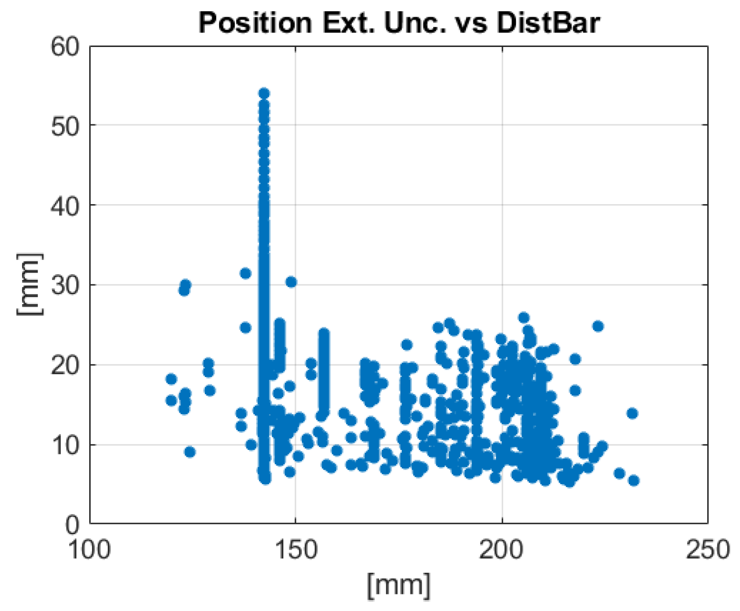
• The mean distance DistBar of the 3D points from their barycenter, see Figure 15f.
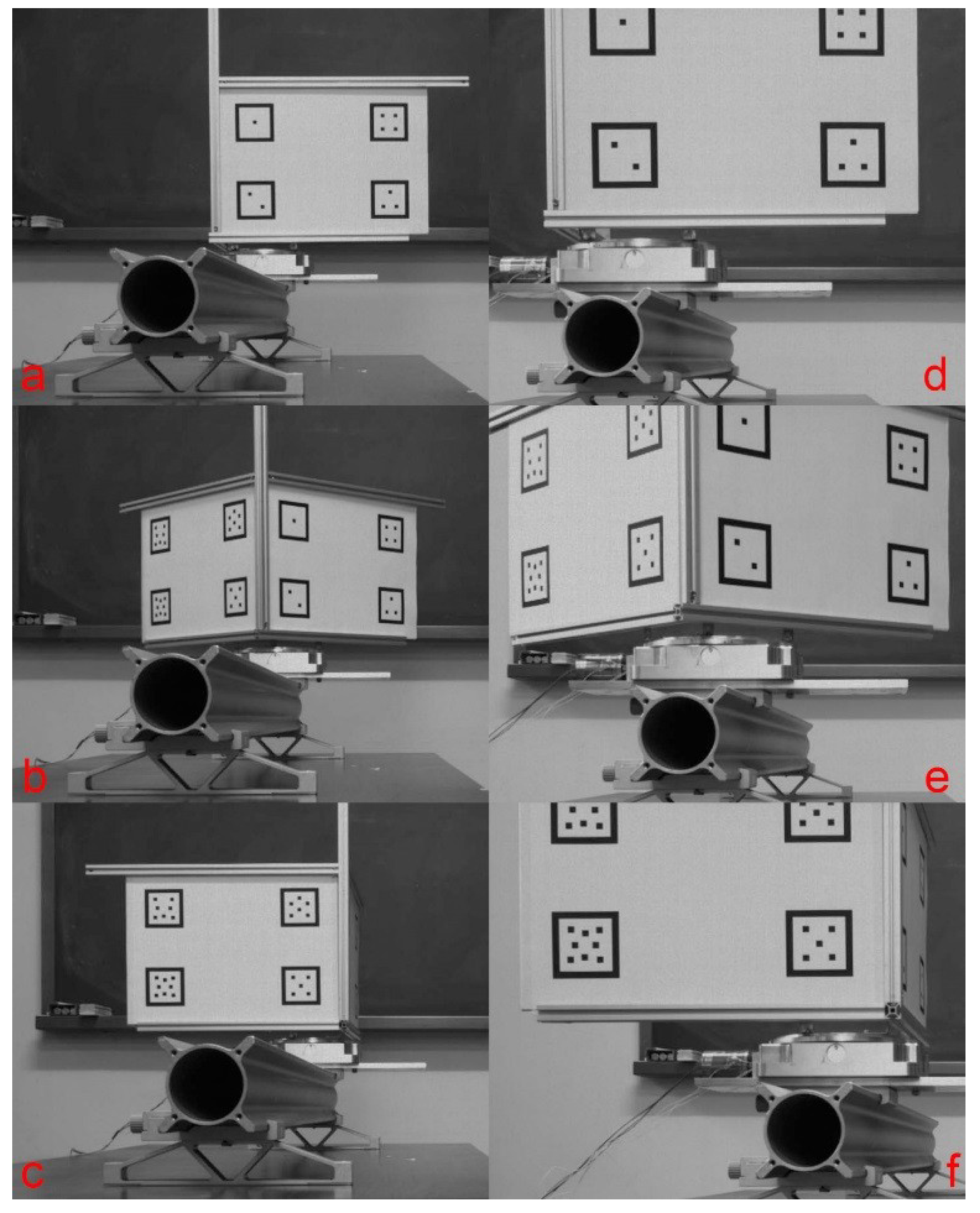
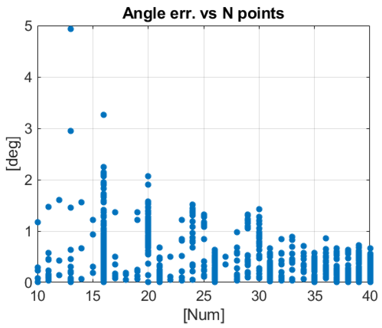
• The number N_points of 2D points observed in each image that pass the RANSAC selection. The number N_points takes into account both the observability of the markers, which is generally lower at short distances (see Figure 7d–f) or when only one face of the mock-up is visible (see Figure 7a,c,d,f), and the consensus set yielded by the RANSAC procedure.
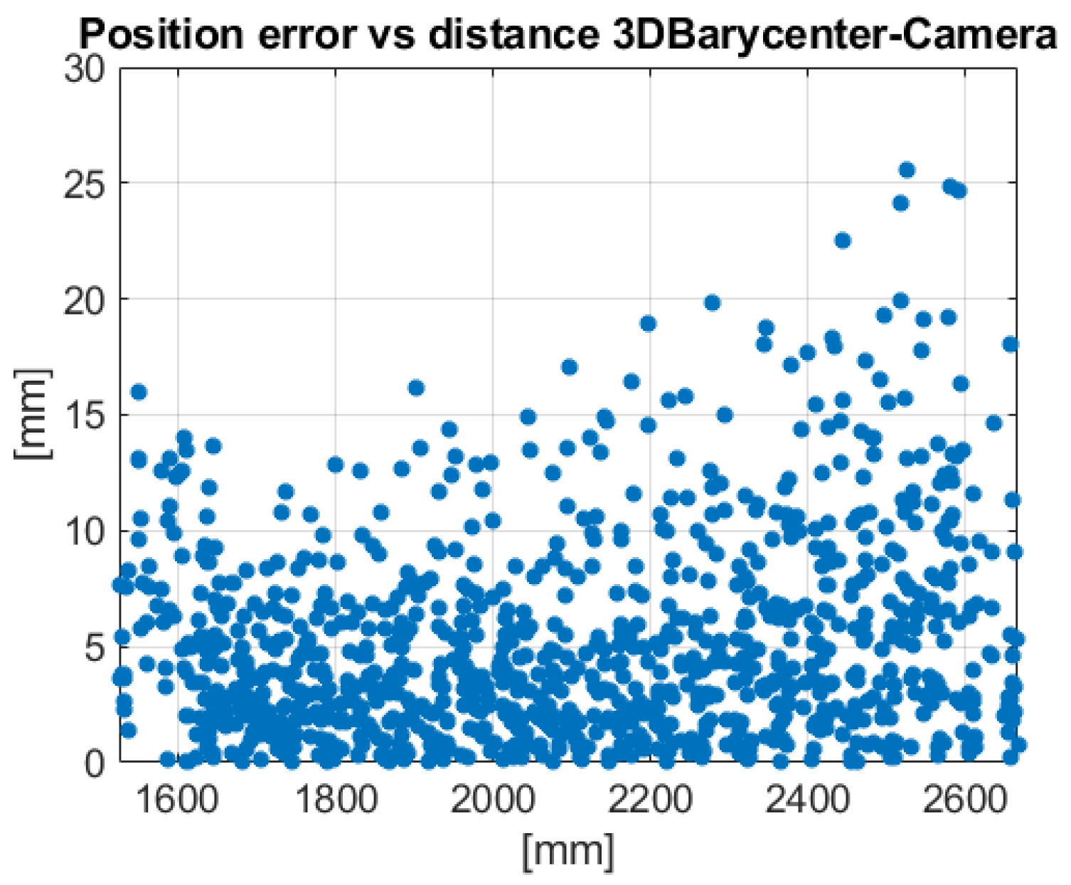
• The distance Dist_BC between the camera (the origin of the C frame) and the barycenter of the 3D points that pass the RANSAC selection.

The interest in the angular parameters α₂ and α₃ comes from the theory of the projective geometry: if a 3D point moves along its projection line, i.e., its local velocity is parallel to its projection line, its movement cannot be observed by the camera, and in this case the measurement error should be large. This theoretical reasoning leads to the preference of high values of α₂ and α₃. The direction of the local velocity can be easily detected in our set-up since the rotation is imposed along a known rotation axis by the rotary stage and the displacement is along the linear slide, but in a general motion, the parameters α₂ or α₃ could be difficult to evaluate. Thus, the simplified parameters α and β were conceived. LongZ, TransvX, and DistBar are parameters that characterize the dispersion of the 3D points. If the 3D points are far from each other and the satellite is rotating around an axis near its barycenter, even a small rotation will yield significant displacement of the 3D points and the rotation angle will be easily evaluated with a low error. Thus, the theoretical rationale behind the dispersion parameters LongZ, TransvX, and DistBar is that they could be correlated with the rotation errors and uncertainties. The distance Dist_BC is selected since and far 3D points are observed with large position uncertainty. Thus, Dist_BC could be correlated with the position errors. The number of points N_points is introduced since its higher values are generally associated with lower errors in the solution of PnP problems.

For each one of the 990 positions and orientations examined, the eight parameters already defined are evaluated. Then, the Pearson correlation coefficient between the obtained angle and distance measurement errors and uncertainties, and the eight considered parameters are calculated, to find out if there is any positive or negative correlation between them and to highlight the most influencing parameters. The following

Table 1. The Pearson Correlation Coefficients for the following output results: Rotation Errors (RE) or Incremental Rotation Errors (dRE); Rotation (Extended) Uncertainties (RU) or Incremental Rotation (Extended) Uncertainties (dRU); Position Errors (PE); Position (Extended) Uncertainties (PU).

	Influencing Parameters
	1/α	β	1/LongZ	1/α2	1/DistBar	1/Npoints	TransvX	DistBC
RE/dRE	0.54	−0.50	0.47	0.36	0.36	0.34	−0.29	0.04
	1/α	β	LongZ	1/Npoints	1/DistBar	1/α2	TransvX	DistBC
RU/dRU	0.87	−0.71	−0.65	0.61	0.60	0.53	−0.50	−0.02
	LongZ	β	α	DistBC	1/DistBar	Npoints	TransvX	1/α3
PE	−0.30	−0.26	−0.22	0.20	0.17	−0.17	−0.16	0.08
	1/α	LongZ	β	1/α3	1/DistBar	Npoints	TransvX	DistBC
PU	0.79	−0.64	−0.64	0.48	0.48	−0.44	−0.34	0.26

summarizes the most significant results: each column considers a parameter or its reciprocal value. The analysis considers the evaluated values of each parameter to find out if there is a linear correlation between the achieved errors or uncertainties and the considered parameter. At the same time, the reciprocal values of each parameter are evaluated to find out if there is a hyperbolic correlation. Each row of Table 1 shows a different output result: Rotation Errors (RE) or Incremental Rotation Errors (dRE); Rotation (Extended) Uncertainties (RU) or Incremental Rotation (Extended) Uncertainties (dRU); Position Errors (PE); Position (Extended) Uncertainties (PU). For the rotation angles, both the total rotation measurements, which varies between 0 and 90°, and the incremental rotation measurements are analyzed; in Table 1, only the most significant case (total or incremental) is reported. For each row, the parameters are ordered from the most significant (first column on the left) to the least significant (last column on the right). For each output result (each row), the three most influencing parameters are highlighted.

Table 1 gives a clear and coherent idea of the most influencing parameters. For all the output results (the rotation errors and uncertainties, the position errors and uncertainties) the three most important parameters are the same: the two mean angles α and β, and the maximum longitudinal distance of the observed 3D points. The angles α and β take into account the mean inclination between the marker plane and the projection line or the optical axis, respectively; see Figure 15a,b. This result highlights that the achievable errors and uncertainties are lower (better) if the mean angles α and β are higher. This conclusion is true for the considered values of α and β, which vary between 0° and 50~60° in the experimental test, as depicted in Figure 16, Figure 17, Figure 18, Figure 19, Figure 20, Figure 21, Figure 22 and Figure 23. Thus, in the design of a measurement system based on markers, a clear indication is to select the satellite surfaces for the markers in order to maximize those two mean angles α and β. This means that the obtained errors and uncertainties are better if the markers are inclined, and not orthogonal, with reference to the projection lines and/or optical axis. Nothing sure can be said if the markers tend to be parallel to the projection lines and/or optical axis since the maximum α and β achieved in the described tests are about 50~60°. A second clear indication is to select the marker positions to maximize the longitudinal distance among them.

Since the Pearson correlation coefficients give a concise but partial representation of a possible correlation between and two quantities, in the following sections, the rotation and/or position errors and/or extended uncertainties are graphically depicted versus each considered parameter. The graphical representation could highlight correlations in a more general way. Section 7.1, Section 7.2, Section 7.3, Section 7.4, Section 7.5, Section 7.6, Section 7.7 and Section 7.8 analyze each parameter at a time, to search for possible correlations not highlighted by the correlation coefficient or to confirm the findings of Table 1.

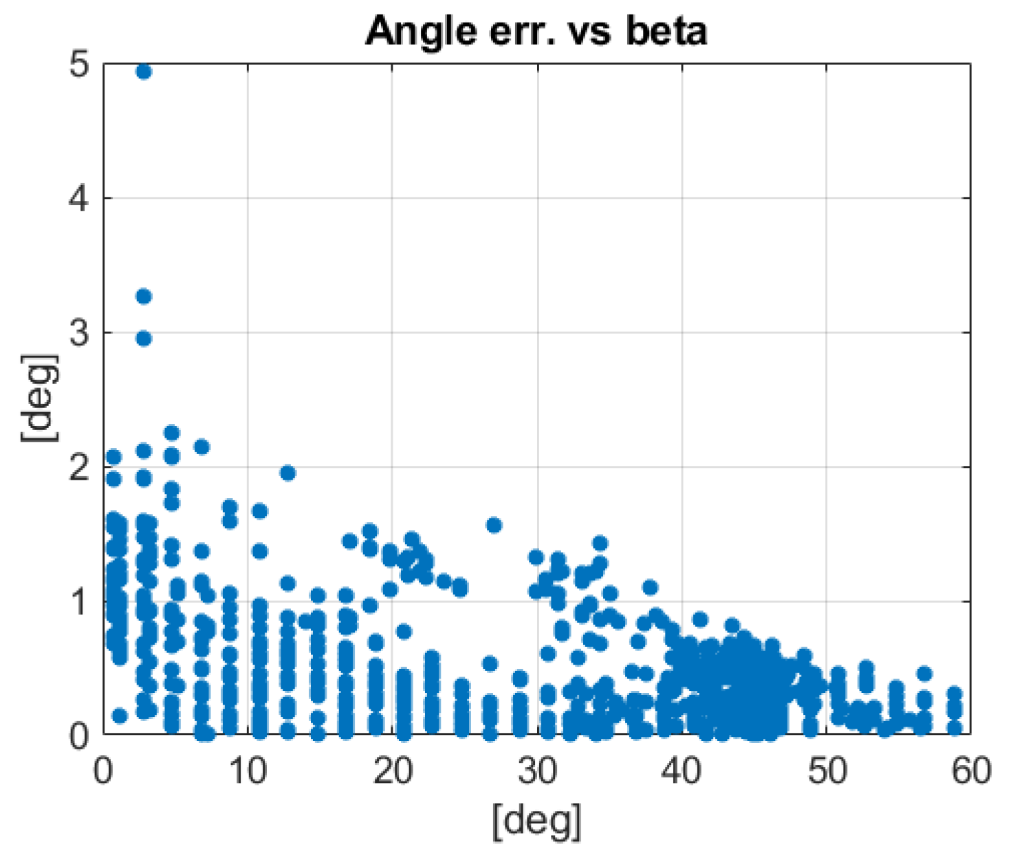
7.1. Parameter a: Mean Angle β

According to Table 1, the mean angle β is the second most influencing parameter in three cases (rows) out of four. In all the four cases (rows) of Table 1, the correlation is more significant with β values and not their reciprocal ones. Thus, the correlation coefficient indicates that a linear correlation is more evident than a hyperbolic one. These findings are confirmed by Figure 16 (rotation errors vs. β) and Figure 18 (rotation extended uncertainties vs. β), while Figure 17 (rotation extended uncertainties vs. β) seems to suggest an intermediate behavior between linear and hyperbolic.

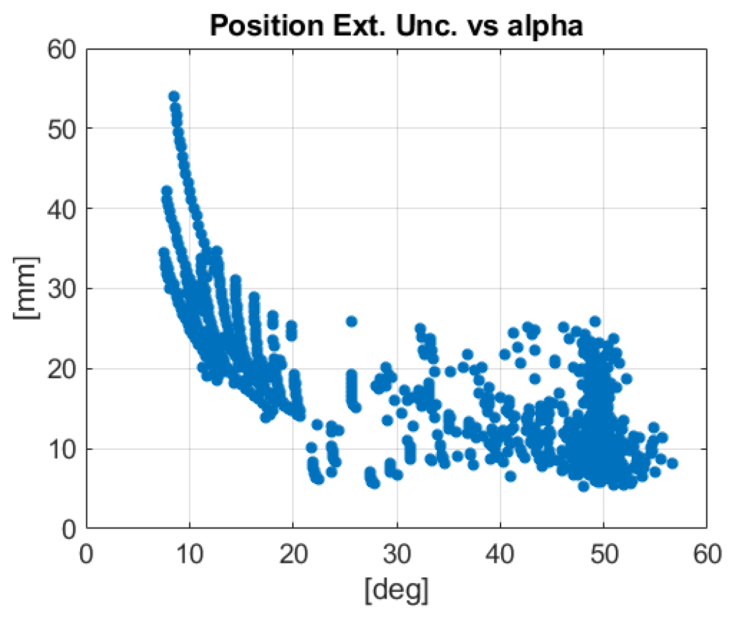
7.2. Parameter b: Mean Angle α

In three rows, out of four, of Table 1, the highest values of the correlation coefficient are obtained for the mean angle α, between each projection line and the normal to the marker plane. The absolute highest value of the correlation coefficient is achieved between the rotation extended uncertainties and the reciprocal values of angles α. Figure 20 depicts this best correlation case and graphically confirms a hyperbolic behavior. Figure 19 shows the incremental rotation errors, while Figure 21 depicts the case of the position extended uncertainties. In all the Figure 19, Figure 20 and Figure 21, there is a hyperbolic increase of the errors and uncertainties when the angle α decreases. Both Table 1 and Figure 19, Figure 20 and Figure 21 suggest that the correlation between errors/uncertainties and α is slightly stronger than in the case of β. Figure 22 shows the angles α, β and the number of points N_points (see Section 7.7) versus the imposed rotation angle; in each imposed rotation angle, the depicted value is averaged for all the 22 positions. Taking into account Figure 22 and the strong correlation between α and the rotation errors and uncertainties, the reduction of angular error and uncertainty near 45–50° (of the imposed rotation), observed in Figure 11 in Section 6, can be understood: for the central angular positions near 45–50°, when the observed surfaces of the satellite mock-up are both inclined (see Figure 7b,e), the angles α and β reach their maximum values and the obtained errors and uncertainties are lower. This a clear indication for the position selection of the fiducial markers on a satellite surface.

Figure 22 shows that the mean number of points N_points remains near 16 points up to an imposed rotation equal to 18°, and near 20 between 86 and 90°. Comparing Figure 11 and Figure 22, and observing only the ranges 0–18° and 86–90° of the imposed angle, there is an evident error and uncertainty variation in and presence of a sensible variation of the mean angles α and β, while the mean number of pairs (${}^{C}x{}_{k,i}$, ${}^{S}X{}_i$) remain constant. However, since the shape of the depicted curve of N_points (versus the imposed rotation) is similar to the corresponding curves of α and β in Figure 22, and since it is generally accepted that an increase of the number of points improves the final results, the doubt that the observed error reduction near 45–50° is due to the number of points and is not associated with the values α and β could legitimately rise. To clarify this doubt, the whole analysis is repeated imposing that the total number of points N_points is lower than 14. This limitation is achieved in the RANSAC procedure imposing that the consensus set cannot have more than 14 pairs (${}^{C}x{}_{k,i}$, ${}^{S}X{}_i$). Since in the analyzed images the minimum number available points is always larger than 14, the effect of the consensus set limitation is that the number of points N_points is constant and does not change. Figure 23 compares the parameters α, β and the RMS error of the attitude angle, all obtained with the number of points N_points kept constant and equal to 14. In this way, the effect of N_points is removed from the analysis. It is clear that the correlation between α, β, and the RMS angular error highlighted by Figure 11 and Figure 22, with N_points variable, is very similar and still evident in the case of Figure 23, without the effect of N_points. Figure 24 compares the RMS error of the attitude angle evaluated considering all the 22 positions, in the case with variable N_points (changing between 15–16 to 38) and in the case with constant N_points (equal to 14). It is clear that the error is generally lower in the case with all points. To conclude, from Figure 22, Figure 23 and Figure 24, both parameters α/β and N_points can be exploited to improve the final measurement error. A possible explanation of the results illustrated in Figure 11, Figure 16, Figure 17, Figure 18, Figure 19, Figure 20, Figure 21, Figure 22, Figure 23, Figure 25 and Figure 26 is that, in our experimental set-up, a rotation of the target spacecraft yields larger movements of the 2D projected points if the mean angles α, β, and α₂ are high. Larger movements for the same rotation mean that the imposed angular displacement is better observed by the vision system and the final measurement errors and uncertainties are lower. For high values of the angles α, β, and α₂, the positive effect of larger observed movements is mitigated and balanced by the negative effect of the projective deformation of the markers, which increases the uncertainty of the detected 2D points. This second negative effect with high values of the angles α, β, and α₂ is not evident in the presented analysis since their maximum values are limited. The same explanation of larger movements of the projected points is also valid for the following parameters LongZ and TansvX as described at the end of Section 7.5.

Coming back to the analysis with all points and looking at Figure 22, it can be verified that up to 18°and between 86 and 90°, all the detected points belong to a planar face of the satellite mock-up. Someone may argue that, in and presence of coplanarity among the 3D points, the homography transformation could be exploited, instead of the P3P solution. A selective employment of the homography transformation could be the subject of an interesting future investigation, but it is beyond the purpose of the present work. The same authors of the selected closed-form and direct solution of the P3P problem, [16], do not highlight any degenerate coplanar configuration of the 3D points. Moreover, in Figure 11, comparing the angular ranges with coplanarity (0–18° and 86–90°) and without coplanarity (20–84°), there is not an evident discontinuity of the obtained errors and uncertainties. Thus, from Figure 11 and Figure 22, even if an effect of coplanarity cannot be excluded, other factors (e.g., the mean angles α and β) appear more important and influencing for the final errors and uncertainties.

7.3. Parameter c: Mean Angles α₂ and α₃

The correlation coefficients of Table 1 obtained in the case of the mean angles α₂ and α₃ are less significant than the other two mean angles α and β. However, all the following Figure 25, Figure 26 and Figure 27 show a clear error/uncertainty increase when α₂/α₃ decreases. Moreover, from a theoretical point of view, the angular distance between the projection line and the local/tangential velocity (considered in α₂ and α₃), instead of the marker plane (considered in α and β), should be significant for incremental rotations or displacements since the motion of a 2D point cannot be observed if its angle α₂/α₃ is equal to zero (the considered 2D point moves along the projection line and its position in the image does not change). These observations lead to the indication that the angles α₂ and α₃ are also significant and should be taken into account in the design of a measurement system based on markers.

7.4. Parameter d: Maximum Longitudinal Distance LongZ

The maximum longitudinal distance of the 3D points is the third most influencing parameter if the correlation coefficients of Table 1 are considered. The following Figure 28 and Figure 29 depict respectively the rotation and position extended uncertainties versus the parameter LongZ and confirm a clear negative correlation between them.

7.5. Parameter e: Maximum Transverse Distance TransvX

The maximum transverse distance among the 3D points exhibits the second least significant correlation coefficient in all the four rows of Table 1. Figure 30 shows the angle error versus the parameter TransvX and confirms that there is no linear or hyperbolic correlation between them. The effect of the transversal distribution of 3D points appears substantially different from the longitudinal one. From Figure 30, it is clear that both low and high values of TransvX are associated with low angular errors, while the higher errors take place when TransvX takes intermediate values. The different behavior of the two parameters LongZ and TransvX (as highlighted by the values of the correlation coefficients and by Figure 28 vs. Figure 30) can be explained considering the observed movements of the 2D projected points. If the 3D points (markers) are dispersed and spaced out along the longitudinal direction, a rotation (around an axis roughly orthogonal to the longitudinal optical axis as in the experimental set-up and near the 3D point barycenter) yields transverse displacements of the 3D points and larger observed movements of the projected 2D points than the case with 3D points dispersed along a transverse direction. Larger 2D observed movements allow us to obtain lower errors and uncertainties in the rotation measurement.

7.6. Parameter f: Mean Distance DistBar of the 3D Points from Their Barycenter

The parameter DistBar, which is the mean distance between the 3D points and their barycenter (Figure 15f), does not excel for its correlation coefficients in Table 1. This low correlation is graphically confirmed by Figure 31 which illustrates the case of the position extended uncertainties and shows that all possible uncertainty values are possible with the same value of DistBar (see the vertical line). However, if the rotations are considered, Figure 32 shows that the angular errors exhibit a slight negative correlation with DistBar: the longitudinal motion does not seem affected by DistBar in a general and evident way, while the rotation errors increase if DistBar gets lower.

7.7. Parameter g: Number of Points N_points

Both in Table 1 and in the following Figure 33 and Figure 34, the number of points N_points exhibits an effect very similar to the parameter DistBar: no evident correlation with the position and a slight negative correlation with the rotation. Figure 22, Figure 24 and Figure 33 illustrate a slight correlation with the final angular errors and their uncertainties, as in Table 1, confirming the generally accepted belief that an increase of N_points reduces the final error. A possible effect of the spatial distribution (with/without coplanarity), when N_points is low, has been already discussed in Section 7.2.

7.8. Parameter h: Distance Dist_BC Barycenter—Camera

In Table 1, the distance between the point barycenter and the camera is the least significant parameter in three out of four cases (rows). However, both Figure 14 of Section 6 and the following Figure 35 and Figure 36, highlight a slight positive correlation which cannot be detected only from the correlation coefficient (except in the position error case, summarized in the third row of Table 1): if the observed target gets farther, the errors and uncertainties increase. Looking at Figure 36, the position uncertainties are aligned along lines almost straight and each line corresponds to a different inclination of the spacecraft. The best line, i.e., with the lowest uncertainty increment for the same distance variation, exhibits an inclination roughly equal to 4 mm/m. This means that an increment of 1 m in the camera-satellite distance yields an uncertainty increase of 4 mm. The worst case has an inclination of 21 mm/m, while the average inclination, which can be evaluated from Figure 14, is roughly 8 mm/m. We warn that these results are obtained with a limited total distance variation of about 1.05 m and that any extrapolation could be dangerous.

As already said in Section 6, this behavior seems reasonable and coherent with the reduction of the observed size of the markers when the distance increases.

8. Conclusions

An improved approach based on a single camera and fiducial markers for the measurement of the relative pose between a target and a chaser spacecraft is presented and described. The measurement procedure integrates a closed-form solution of the PnP problem, a RANSAC procedure, a non-linear local optimization, and a global Bundle Adjustment refinement of both the measured poses and the 3D point map. The employed experimental set-up allows us a metrological characterization and the evaluation of the measurement errors, while a Monte Carlo analysis allows us to evaluate the position and rotation uncertainties. The application of the method to an experimental data set acquired in laboratory highlights the significant improvements provided by the Bundle Adjustment refinement. A set of possible influencing physical parameters are defined and their correlations with the rotation and position errors and uncertainties are analyzed. Using both numerical quantitative correlation coefficients and qualitative graphical representations, the most significant parameters for the final measurement errors and uncertainties are found out. In detail, the mean angle α between each projection line of the 3D points and the normal to the marker planes resulted in the most influencing parameter, whose maximum values around 50 deg exhibit the best uncertainty and the lowest errors. The obtained results give clear indications and advice for the design of future measurement systems and for the selection of the marker positioning on a satellite surface.

References

1. Mokuno, M.; Kawano, I. In-orbit demonstration of an optical navigation system for autonomous rendezvous docking. AIAA J. Spacecr. Rockets 2011, 48, 1046–1054. [Google Scholar] [CrossRef]
2. Howard, R.; Heaton, A.; Pinson, R.; Carrington, C. Orbital Express Advanced Video Guidance Sensor. In Proceedings of the 2008 IEEE Aerospace Conference, Big Sky, MT, USA, 1–8 March 2008. [Google Scholar]
3. Howard, R.T.; Heaton, A.F.; Pinson, R.M.; Carrington, C.L.; Lee, J.E.; Bryan, T.C.; Robertson, B.A.; Spencer, S.H.; Johnson, J.E. The Advanced Video Guidance Sensor: Orbital Express and the next generation. In AIP Conference Proceedings; AIP: College Park, MD, USA, 2008; Volume 969, pp. 717–724. [Google Scholar]
4. Bodin, P.; Noteborn, R.; Larsson, R.; Karlsson, T.; D’Amico, S.; Ardaens, J.S.; Delpech, M.; Berges, J.C. PRISMA formation flying demonstrator: overview and conclusions from the nominal mission. Adv. Astronaut. Sci. 2012, 144, 441–460. [Google Scholar]
5. Tweddle, B.E. Relative Computer Vision Based Navigation for Small Inspection Spacecraft. In Proceedings of the AIAA Guidance, Navigation and Control Conference, Portland, OR, USA, 8–11 August 2011. [Google Scholar]
6. Tweddle, B.E.; Saenz-Otero, A. Relative Computer Vision-Based Navigation for Small Inspection Spacecraft. J. Guid. Control Dyn. 2014, 38, 969–978. [Google Scholar] [CrossRef]
7. Sansone, F.; Branz, F.; Francesconi, A. A Relative Navigation Sensor for Cubesats Based on Retro-reflective Markers. In Proceedings of the International Workshop on Metrology for Aerospace, Padua, Italy, 21–23 June 2017. [Google Scholar]
8. Pertile, M.; Mazzucato, M.; Chiodini, S.; Debei, S.; Lorenzini, E. Uncertainty evaluation of a vision system for pose measurement of a spacecraft with fiducial markers. In Proceedings of the International Workshop on Metrology for Aerospace, Benevento, Italy, 4–5 June 2015. [Google Scholar]
9. Lepetit, V.; Moreno-Noguer, F.; Fua, P. EPnP: An Accurate O(n) solution to the PnP problem. Int. J. Comput. Vis. 2009, 81, 155–166. [Google Scholar] [CrossRef] [Green Version]
10. Ma, Y.; Soatto, S.; Kosecka, J.; Sastry, S.S. An Invitation to 3-D Vision; Springer Science & Business Media: Berlin, Germany, 2004. [Google Scholar]
11. Hartley, R.; Zisserman, A. Multiple View Geometry in Computer Vision, 2nd ed.; Cambridge University Press: New York, NY, USA, 2004. [Google Scholar]
12. Haralick, R.; Lee, C.; Ottenberg, K.; Nolle, M. Review and Analysis of Solutions of the Three Point Perspective Pose Estimation Problem. Int. J. Comput. Vis. 1994, 13, 331–356. [Google Scholar] [CrossRef]
13. Quan, L.; Lan, Z. Linear N-point camera pose determination. IEEE Trans. Pattern Anal. Mach. Intell. 1999, 21, 774–780. [Google Scholar] [CrossRef] [Green Version]
14. Gao, X.; Hou, X.; Tang, J.; Cheng, H. Complete solution classification for the perspective-three-point problem. IEEE Trans. Pattern Anal. Mach. Intell. 2003, 25, 930–943. [Google Scholar]
15. Nister, D.; Stewenius, H. A minimal solution to the generalized 3-point pose problem. J. Math. Imaging Vis. 2006, 27, 67–79. [Google Scholar] [CrossRef]
16. Kneip, L.; Scaramuzza, D.; Siegwart, R. A Novel Parametrization of the Perspective-Three-Point Problem for a Direct Computation of Absolute Camera Position and Orientation. In Proceedings of the IEEE Conference on Computer Vision and Pattern Recognition, CVPR 2011, Colorado Springs, CO, USA, 20–25 June 2011. [Google Scholar]
17. Christian, J.A.; Robinson, S.B.; D’Souza, C.N.; Ruiz, J.P. Cooperative Relative Navigation of Spacecraft Using Flash Light Detection and Ranging Sensors. J. Guid. Control Dyn. 2014, 37, 452–465. [Google Scholar] [CrossRef]
18. Opromolla, R.; Fasano, G.; Rufino, G.; Grassi, M. A review of cooperative and uncooperative spacecraft pose determination techniques for close-proximity operations. Prog. Aerosp. Sci. 2017, 93, 53–72. [Google Scholar] [CrossRef]
19. Jeong, J.; Kim, S.; Suk, J. Parametric study of sensor placement for vision-based relative navigation system of multiple spacecraft. Acta Astronaut. 2017, 141, 36–49. [Google Scholar] [CrossRef]
20. Yousefian, P.; Durali, M.; Jalali, M.A. Optimal design and simulation of sensor arrays for solar motion estimation. IEEE Sens. J. 2017, 17, 1673–1680. [Google Scholar] [CrossRef]
21. Jackson, B.; Carpenter, B. Optimal placement of spacecraft sun sensors using stochastic optimization. In Proceedings of the IEEE Aerospace Conference, Big Sky, MT, USA, 6–13 March 2004; Volume 6, pp. 3916–3923. [Google Scholar]
22. Kato, H.; Billinghurst, M. Marker tracking and HMD calibration for a video-based augmented reality conferencing system. In Proceedings of the 2nd IEEE and ACM International Workshop on Augmented Reality, IWAR 099, IEEE Computer Society, Washington, DC, USA, 20–21 October 1999; pp. 85–94. [Google Scholar] [Green Version]
23. Garrido-Jurado, S.; Muñoz-Salinas, R.; Madrid-Cuevas, F.J.; Marín-Jiménez, M.J. Automatic generation and detection of highly reliable fiducial markers under occlusion. Pattern Recognit. 2014, 47, 2280–2292. [Google Scholar] [CrossRef]
24. Ahn, S.J.; Warnecke, H.J.; Kotowski, R. Systematic Geometric Image Measurement Errors of Circular Object Targets: Mathematical Formulation and Correction. Photogramm. Rec. 1999, 16, 485–502. [Google Scholar] [CrossRef] [Green Version]
25. Zhang, Z. A Flexible New Technique for Camera Calibration. IEEE Trans. PAMI 2000, 22, 1330–1334. [Google Scholar] [CrossRef]
26. Gonzalez, R.C.; Woods, R.E.; Eddins, S.L. Digital Image Processing Using MATLAB; Pearson Prentice Hall: Upper Saddle River, NJ, USA, 2004. [Google Scholar]
27. Heckbert, P.S.; Garland, M. Survey of Polygonal Surface Simplification Algorithms; Multiresolution Surface Modeling Course SIGGRAPH 97, Carnegie Mellon University Technical Report; Carnegie Mellon University School of Computer Science: Pittsburgh, PA, USA, 1997. [Google Scholar]
28. Fischler, M.A.; Bolles, R.C. Random sample consensus: a paradigm for model fitting with applications to image analysis and automated cartography. Commun. ACM 1981, 24, 381–395. [Google Scholar] [CrossRef] [Green Version]
29. Moré, J.J. The Levenberg-Marquardt Algorithm: Implementation and Theory. In Numerical Analysis; Lecture Notes in Mathematics 630; Watson, G.A., Ed.; Springer: Berlin, Germany, 1977; pp. 105–116. [Google Scholar]
30. Lourakis, M.I.A.; Argyros, A.A. SBA: A Software Package for Generic Sparse Bundle Adjustment. ACM Trans. Math. Softw. 2009. [Google Scholar] [CrossRef]
31. Triggs, B.; McLauchlan, P.; Hartley, R.; Fitzgibbon, A. Bundle Adjustment: A Modern Synthesis. In International Workshop on Vision Algorithms; Springer: Berlin/Heidelberg, Germany, 1999; pp. 298–372. [Google Scholar]
32. BIPM; IEC; IFCC; ILAC; ISO; IUPAC; IUPAP; OIML. Evaluation of Measurement Data—Guide to the Expression of Uncertainty in Measurement; International Organization for Standardization: Geneva, Switzerland, 2008. [Google Scholar]
33. BIPM; IEC; IFCC; ILAC; ISO; IUPAC; IUPAP; OIML. Evaluation of Measurement Data—Supplement 1 to the Guide to the Expression of Uncertainty in Measurement—Propagation of Distributions Using a Monte Carlo Method; International Organization for Standardization: Geneva, Switzerland, 2008. [Google Scholar]
Figure 1. Scheme of the whole measurement procedure.
Robotics 07 00043 g001
Figure 2. The scheme of steps. (step A) the detection of 2D marker points and (step B) the P3P solution inside RANSAC.
Robotics 07 00043 g002
Figure 3. (a) The detection of 2D points in each acquired image; (b) the vertices of the markers.
Robotics 07 00043 g003
Figure 4. The scheme of the steps; (step C) the local refinement with non-linear optimization and (step D) the global refinement with BA.
Robotics 07 00043 g004
Figure 5. The scheme of the second implementation of the BA approach.
Robotics 07 00043 g005
Figure 6. The laboratory set-up.
Robotics 07 00043 g006
Figure 7. The images acquired in different positions and rotations: (ac) with maximum distance and rotation angles, respectively, 0, 45, and 90°; (df) with the minimum distance (partial occlusion of the markers) and rotation angles, respectively, 0, 45, and 90°.
Robotics 07 00043 g007
Figure 8. The evaluated attitude angle versus the imposed rotation for a single position along the linear slide: obtained by the Kneip solution (blue); by the Gao solution (orange line); by the EPnP solution (yellow line).
Robotics 07 00043 g008
Figure 9. The root mean square (RMS) error of the attitude angle versus the imposed rotation: obtained by the Kneip solution (blue); by the Gao solution (orange line); by the EPnP solution (yellow line); by the non-linear local optimization (step C) after the Kneip solution inside the RANSAC procedure (step B), (purple line); by the first implementation of the BA approach (light blue line); by the second implementation of the BA approach (green line).
Robotics 07 00043 g009
Figure 10. The angular errors, averaged for the 22 distances, versus the rotation angle, obtained with the non-linear approach without BA (blue) and with BA (orange).
Robotics 07 00043 g010
Figure 11. The root mean square (RMS) error of the attitude angle and its extended uncertainty versus the imposed rotation: angular errors without BA (red line with circular dots); extended uncertainties without BA (red shaded area); angular errors WITH BA (blue line with circular dots); extended uncertainties WITH BA (blue shaded area).
Robotics 07 00043 g011
Figure 12. The root mean square (RMS) error of the linear position and its extended uncertainty versus the imposed rotation: position errors without BA (red line with circular dots); extended uncertainties without BA (red shaded area); position errors WITH BA (blue line with circular dots); extended uncertainties WITH BA (blue shaded area).
Robotics 07 00043 g012
Figure 13. The root mean square (RMS) error of the attitude angle and its extended uncertainty versus the imposed position: angular errors without BA (red line with circular dots); extended uncertainties without BA (red shaded area); angular errors WITH BA (blue line with circular dots); extended uncertainties WITH BA (blue shaded area).
Robotics 07 00043 g013
Figure 14. The root mean square (RMS) error of the linear position and its extended uncertainty versus the imposed position: position errors without BA (red line with circular dots); extended uncertainties without BA (red shaded area); position errors WITH BA (blue line with circular dots); extended uncertainties WITH BA (blue shaded area).
Robotics 07 00043 g014
Figure 15. The schematic representation of the parameters af that potentially affect the measurement errors and uncertainties (the yellow square is the top view of the satellite mock-up; the circular red dots are the corners of the square markers; the camera is depicted in red); subplot a represents parameter a (mean angle β), subplot b → parameter b (mean angle α), …, subplot f → parameter f (mean distance DistBar).
Robotics 07 00043 g015
Figure 16. The rotation errors vs. the mean angle β.
Robotics 07 00043 g016
Figure 17. The rotation extended uncertainties vs. the mean angle β.
Robotics 07 00043 g017
Figure 18. The rotation extended uncertainties vs. the mean angle β.
Robotics 07 00043 g018
Figure 19. The incremental rotation errors vs. the mean angle α.
Robotics 07 00043 g019
Figure 20. The rotation extended uncertainties vs. the mean angle α.
Robotics 07 00043 g020
Figure 21. The position extended uncertainties vs. the mean angle α.
Robotics 07 00043 g021
Figure 22. The mean angle α (black), β (red), and the mean number of points Npoints (blue) vs. the imposed rotations.
Robotics 07 00043 g022
Figure 23. The mean angle α (black), β (red), and RMS error of the attitude angle (blue) vs. the imposed rotations, computed with Npoints ≤ 14.
Robotics 07 00043 g023
Figure 24. The RMS error of the attitude angle vs. the imposed rotations, computed using all the available points (orange line) and with Npoints ≤ 14 (blue line).
Robotics 07 00043 g024
Figure 25. The incremental rotation errors vs. the mean angle α2.
Robotics 07 00043 g025
Figure 26. The rotation extended uncertainties vs. the mean angle α2.
Robotics 07 00043 g026
Figure 27. The position extended uncertainties vs. the mean angle α3.
Robotics 07 00043 g027
Figure 28. The rotation extended uncertainties vs. the longitudinal maximum distance LongZ.
Robotics 07 00043 g028
Figure 29. The position extended uncertainties vs. the longitudinal maximum distance LongZ.
Robotics 07 00043 g029
Figure 30. The rotation errors vs. maximum transverse distance TransvX.
Robotics 07 00043 g030
Figure 31. The position extended uncertainties vs. the mean distance DistBar.
Robotics 07 00043 g031
Figure 32. The rotation errors vs. the mean distance DistBar.
Robotics 07 00043 g032
Figure 33. The rotation errors vs. the number of points Npoints.
Robotics 07 00043 g033
Figure 34. The position extended uncertainties vs. the number of points Npoints.
Robotics 07 00043 g034
Figure 35. The position errors vs. the distance barycenter—camera Dist_BC.
Robotics 07 00043 g035
Figure 36. the position extended uncertainties vs. the distance barycenter—camera Dist_BC.
Robotics 07 00043 g036