Perception-Link Behavior Model: Supporting a Novel Operator Interface for a Customizable Anthropomorphic Telepresence Robot

Abstract

A customizable anthropomorphic telepresence robot (CATR) is an emerging medium that might have the highest degree of social presence among the existing mediated communication mediums. Unfortunately, there are problems with teleoperating a CATR, and these problems can deteriorate the gesture motion in a CATR. These problems are the disruption during decoupling, discontinuity due to the unstable transmission and jerkiness due to the reactive collision avoidance. From the review, none of the existing interfaces can simultaneously fix all of the problems. Hence, a novel framework with the perception-link behavior model (PLBM) was proposed. The PLBM adopts the distributed spatiotemporal representation for all of its input signals. Equipping it with other components, the PLBM can solve the above problems with some limitations. For instance, the PLBM can retrieve missing modalities from its experience during decoupling. Next, the PLBM can handle up to a high level of drop rate in the network connection because it is dealing with gesture style and not pose. For collision prevention, the PLBM can tune the incoming gesture style so that the CATR can deliberately and smoothly avoid a collision. In summary, the framework consists of PLBM being able to increase the user’s presence on a CATR by synthesizing expressive user gestures.

1. Introduction

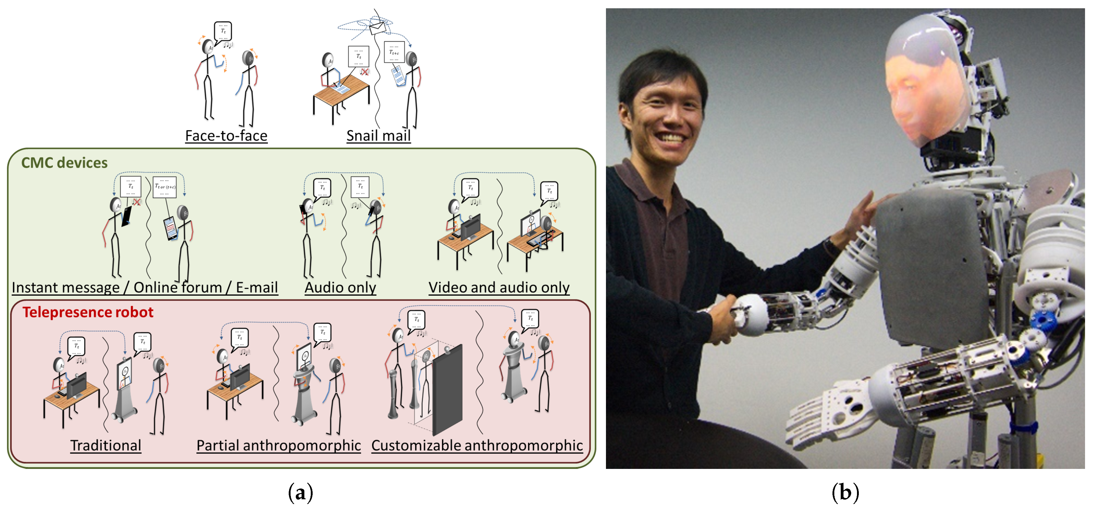
Interpersonal communication is a common way for people to exchange information, and Figure 1a shows the various mediums for transmitting that information. Naturally, face-to-face communication (FTFC) is the golden standard because it has richer social cues, which make the communication process more efficient. These social cues, e.g., facial expression and gestures, can show the degree of intimacy and immediacy towards a person or a topic. Despite the advantages in FTFC, computer-mediated communication (CMC) devices are still essential mediums for the future because the CMC devices have many advantages. For instance, most of the CMC devices support distant communication. However, they have a lower level of social presence when compared to FTFC. Among the emerging CMC devices, the customizable anthropomorphic telepresence robot (CATR) should have the highest level of social presence. The CATR, e.g., EDGAR-1 (Expression Display & Gesturing Avatar Robot) [1] (Figure 1b), has an upper anthropomorphic structure and customizable head module so that it can perform realistic interactive motions and facial expression. With this appearance, the CATR should be the closest to the FTFC in terms of social presence. However, this anthropomorphic appearance must be paired with a lifelike behavior to be efficient.

For this paper, the gesture modality is the central focus because it has many functions and effects on a conversation. For example, the punctuation gesture, also known as the baton gesture [2], can emphasize the important segment of speech. There are also the interactive gestures that regulate and organize a spoken dialog [3]. Furthermore, Neff et al. [4] have shown that the intensity of the gesture correlates with the perception of extroversion. In conclusion, a gesture has many effects and functions during a communication process. Unfortunately, its motion might be affected during the transmission process.

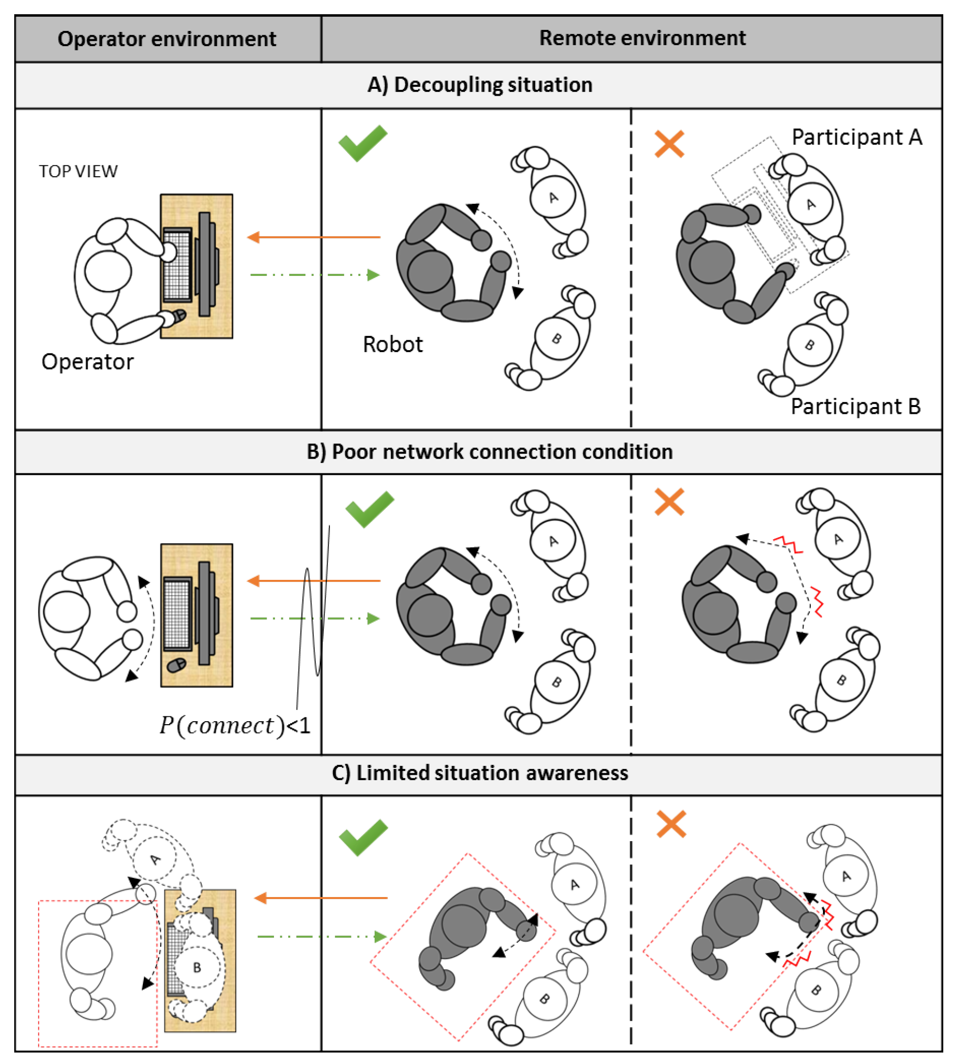
When an operator controls a CATR, there are different situations that might corrupt his/her synthesized gesture motion. They include decoupling, intermittent network connection and reactive collision avoidance (Figure 2). Decoupling [5] happens when the operator commits a part of his/her nonverbal modalities for another task instead of the conversation. An example is when the operator is typing on the keyboard instead of gesturing, and the typing motion is irrelevant to and undesirable for the conversation. Next, the second scenario occurs when the network condition is inconsistent. An intermittent connection might cause jerky and uncanny synthesized gestures. For the last scenario, this happens when there is a lack of situational awareness, and the existing solution [5] is to clip off any out-of-bound motion. This reactive method might affect the smoothness of the motions. In short, an ideal interface must handle the above issues so that the operator can operate the CATR without compromising the conversation.

As a result, the aim of the paper is to study and develop a supporting framework using the perception-link behavior model (PLBM) that is capable of handling the teleoperating issues (Figure 2), which are mentioned in [5,6]. The objectives are as follows:

• The CATR must imitate the operator’s personal gestures.
• The CATR must have an intuitive and easy to use control interface.
• During decoupling, the CATR will generate the operator’s behavior according to the surrounding contexts.
• If the connection is unstable, the CATR will continue to gesticulate smoothly and congruently.
• If the operator motions an out-of-bound gesture, the CATR will
  • not pose any danger to the audience.
  • not distort the intent of the gesture.

2. Related Work

This section presents works related to gesture reconstruction, gesture transmission and multimodal association. Firstly, it will cover the fundamental components that include the input interface, the encoder, the decoder and the associator. Subsequently, it will present the various data representations. The last part will point out the best attribute of the components and a desirable data representation to meet our goals.

First of all, most existing models have four components, and they are the input interface, the encoder, the decoder and the associator. The input interface is the acquisition component that acquires the gesture information from the operator. An example of the input interface is the master-slave system from the MeBot [5]. For this interface, the operator controls the master manipulator, and the slave manipulator imitates the motion. The next component is the encoder that transforms a single/series of joint states into another representation. For instance, the gesture classification module in Park’s model [7] is an encoder. The module can classify the operator’s motion into one of the 13 predefined actions. On the contrary, the decoder extrapolates the future joint state using the new representation. From the same example, Park’s model [7] had a motion generator with 13 predefined motions. The motion generator would execute one of the motions depending on the predicted class. The last component is the associator that learns the relationships between different modalities. None of the telepresence robot interfaces have this component. For instance, the MeBot [5] could display different modalities, e.g., neck, arms, video and audio, but each of the modalities worked independently from the another. In conclusion, the four components cover various processes, such as the acquisition, transformation and association process, which is important in teleoperation. Especially for the transformation process, it remaps the input into another representation that has different properties, which might affect the transmission and the association process.

In this review, there are three representations. They are the local spatiotemporal, distributed spatial and distributed spatiotemporal representation, and their features can be manually coded or automatically extracted. The local spatiotemporal (manual) representation is a list of manually-coded gesture styles, where the winner will take all. For instance, Park’s model [7] has 13 local gesture actions, e.g., lift right, lift left and lift both arms. At any time, the model will select only one of them. On the other hand, the distributed spatial (manual) representation is a set of predefined features that only captures the spatial information. An example is the transmitted signal in MeBot [5], and it is the immediate information of the joints. Lastly, the distributed spatiotemporal (auto) representation is a set of self-extracted features that capture the spatiotemporal information. For Lau’s model [8], a probabilistic model, the dynamic Bayesian network, models an input sequence into a probability distribution, which is the spatiotemporal features. In short, different representations have various properties, such as spatial or spatiotemporal properties. These properties can either solve or impose problems in a teleoperation.

Table 1. Comparison of the existing models with their components and effects, where the gray boxes are the desired attributes and effects. For a detailed description of the attributes, please refer to Supplementary Material 1.

		Components					Effects
		Input Interface	Representation	Encoder	Decoder	Associator	Expressivity	Cognitive Load	Decoupling	Obstacle Avoidance
Telepresence robot	TTR(>100	Traditional	Local spatiotemporal	Manual	Auto	-	High	High	Yes (idle)	Deliberative
	predefined gestures)	input device	(>100 predefined gestures)							and Reactive
	TPR(<10	Traditional	Local spatiotemporal	Manual	Auto	-	Low	Low	Yes (idle)	Deliberative
	predefined gestures)	input device	(<10 predefined gesture)					(require remapping)		and Reactive
	MeBot [5]	Master-slave	Distributed spatial (Manual)	Direct	Direct	-	High	Low	Yes (idle)	Reactive
								(require remapping)
	Hasegawa [10]	Natural interface	Distributed spatial (Manual)	Direct	Direct	-	High	Low	No	Reactive
	Park [7]	Natural interface	Local spatiotemporal	Auto	Auto	-	Low	Auto	Yes (idle)	Deliberative
			(13 predefined gestures)							and Reactive
Virtual agent	Hartmann [11]	Traditional	Distributed	Manual	Auto	Manual	High	High	Yes (associate)	Deliberative
	and Neff [12]	input device	spatiotemporal (Manual)							and Reactive
	Lau [8]	Natural interface	Distributed	Auto	Auto	-	High	Low	Yes (idle)	Deliberative
			spatiotemporal (Auto)							and Reactive
	Taylor [13] (FCRBM)	Natural interface and	Distributed	Manual	Auto	-	High	High	Yes (idle)	Deliberative
	and Xia [14]	Traditional input device	spatiotemporal (Manual)							and Reactive

shows the various components and their attributes (refer to Supplementary Material 1 for a more detail), and the shaded cells are the preferred attributes to overcome the problems. The first property is the spatiotemporal representation with the automatic decoding function. These two components can become a deliberate safety mechanism. With it, a system can tune incoming gestures to avoid any collision; concurrently, it can uphold the gesture expressiveness. Secondly, a good spatiotemporal representation should have distributed and self-extracted features. Unlike local representation, distributed representation can represent new signals and hold more information [9]. Additionally, the automatic feature extractor can produce more consistent and richer distributed features. For satisfying the above requirements with low cognitive load, the system must use the natural interface and the automatic encoder. As a result, the operator directly motions his/her gestures, and the system will encode the sequences into the distributed output for transmission. Finally, the system should have an automatic associator to form rules between different modalities. With the associator, it can substitute inappropriate signal to match the other modalities.

In conclusion, the following configurations, (1) distribution spatiotemporal representation, (2) automatic encoding, decoding and associative module and (3) natural interface, can meet the objectives. Hence, the proposed supporting module, the perception-link behavior model, has the above attributes.

3. Materials and Methods

3.1. Perception-Link Behavior Model

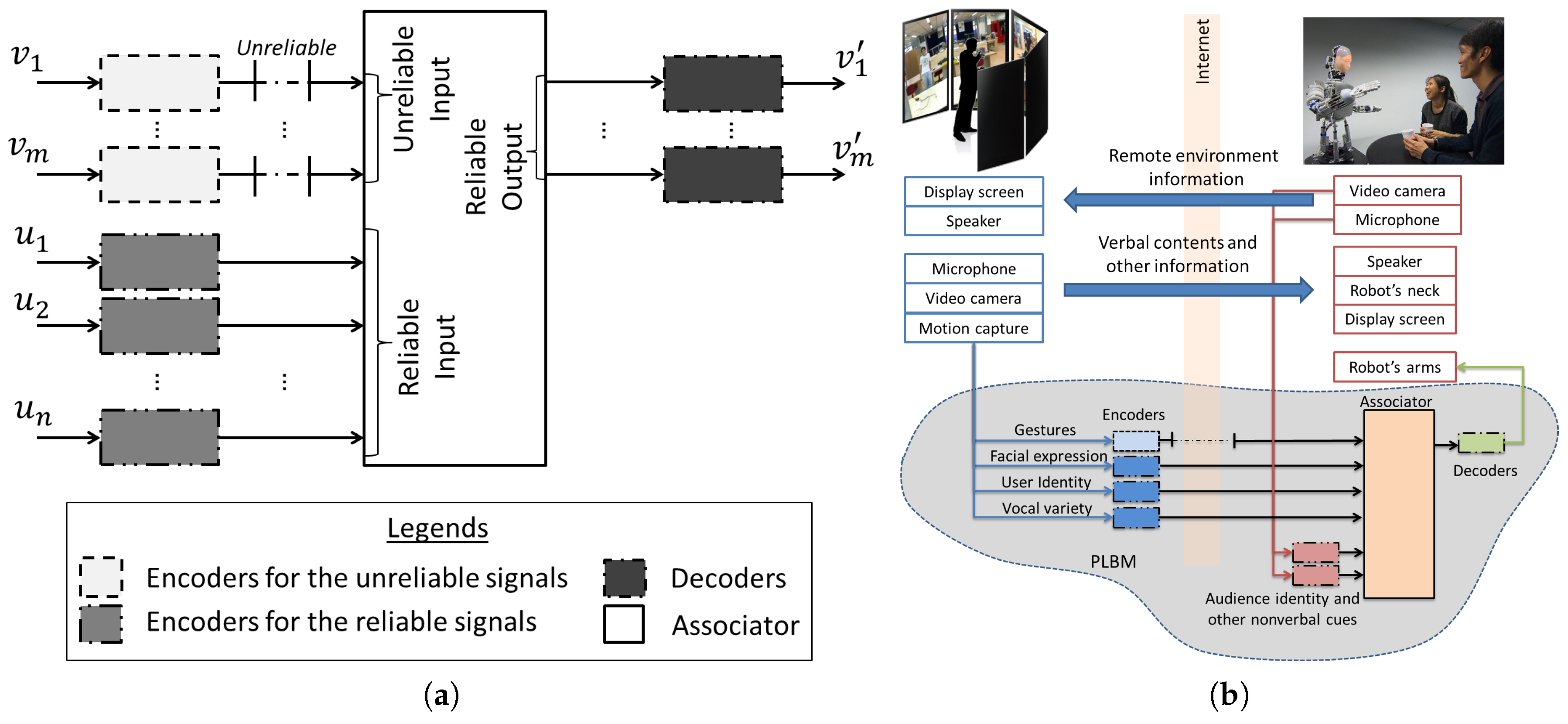
The name of this model is the perception-link behavior model (PLBM) because the conversation partners might react according to what they see during a conversation, and this is the concept behind role negotiation [15] and the chameleon effect [16]. Alternatively, the perception-link behavior model (PLBM) is also an online associative multimodal model with encoding and decoding capability (Figure 3a). It can be implemented into a CATR’s framework to associate multiple modalities, as shown in Figure 3b. Primarily, it has three components: encoders, decoders and associator.

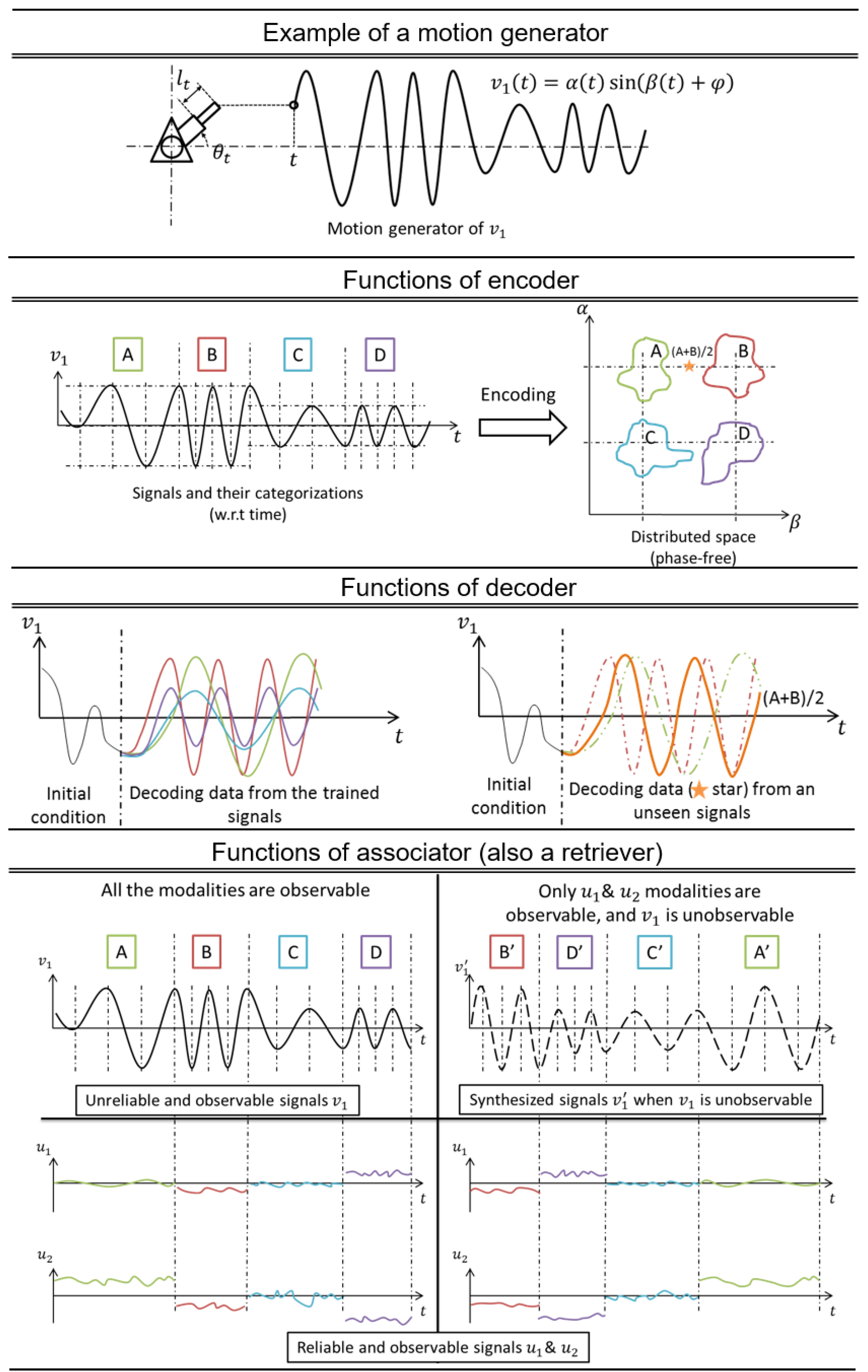
The following descriptions are the function of each component with a simple example. The encoder transforms the input signal into distributed output, and it groups similar signals nearer to each other. For example, let us assume that there exists a motion generator (Figure 4, Row 1) with two degrees of freedom: linear $l_t$ and rotation ${\theta }_t$. During the training process, the motion generator only generated four signals, A, B, C and D, by varying $l_t$ and $\delta {\theta }_t/\delta t$. The encoder should learn the distributed features $\alpha$ and $\beta$ using the training signals. Subsequently, the encoder can map any signal, including $(A+B)/2$, into the new space, as shown in Figure 4, Row 2, where the signals with similar dynamics are grouped nearer to each other. From the distributed output, the decoder should extrapolate the gesture motion without losing its expressiveness. Once the encoder has mapped a signal to its distributed output, the decoder can take the distributed output and transform it back to its originals dynamic (Figure 4, Row 3). Lastly, the associator can learn relationships between multiple modalities. If necessary, it can retrieve the missing signal from its knowledge base. Figure 4, Row 4, left, shows the relationship of a motion $v_1$ and the two other signals $u_1$ and $u_2$. If these relationships are consistent, then the associator can leverage this knowledge and create a list of rules of these relationships. In a different situation (Figure 4, Row 4, right), if there were a missing channel $v_1$, the associator could exploit the knowledge base and retrieve a synthesized signal $v_1^{\prime }$ given the observable signals $u_1$ and $u_2$.

With the above functions, the framework with PLBM can obtain the first objective of the paper, because it adopts an unsupervised learning model and a contextual generative model. The encoder utilizes an unsupervised learning model so that the extracted features are more thorough and comprehensive. In an unsupervised approach, e.g., Fourier transformation, the distributed features are the amplitude $\alpha$ and angular frequency $\beta$ (Figure 4). However, there is no assurance of the completeness of the features if they are manually selected. Secondly, the model produces distributed features. The distributed representation encompasses more information given the same amount of memory size. For a memory size of N capacity, a system with the distributed binary representation can hold up to $2^N$ classes. On the other hand, the local representation can only group up to N classes. Lastly, the decoder is a contextual generative model that reconstructs the signals given a contextual information, e.g., encoded data. A decoder model predicts a sequence of future time steps ${{\mathit{i}}^{\prime }}_{t:(t+T)}$ given the encoded data ${\mathit{z}}_t\in {\mathrm{R}}^N$ and the boundary conditions ${\mathit{i}}_{(t-p):(t-1)}$. With extensive training, the decoder model should figure out the intrinsic dynamics encompassed in the encoded data ${\mathit{z}}_t$, and it should be capable of generating output ${{\mathit{i}}^{\prime }}_{t:(t+T)}$ similar to the training data ${\mathit{i}}_{t:(t+T)}$. In short, the framework with the PLBM can imitate the operator’s personal gestures because the encoding process preserves expressiveness, and the decoding process is capable of generating personal gestures given the encoded data.

From the review, the framework with the PLBM and natural interface (NI) should result in minimum cognitive load and be easier for the operator to use because they require minimal remapping and less memorization. The NI is the user interface that directly acquires the conversational gesture. For example, Hasegawa [10] chose the NI, instead of the passive model controller [5], because it could capture both conscious and subconscious gestures. From the review, the NI can capture the subconscious gesture because it does not require much remapping. Secondly, the NI also requires less memorization. For our case, we chose the NI because any operator can just make his/her gestures as if it were a face-to-face conversation. Furthermore, all of the modules in the PLBM are automatic. The encoder will automatically encode the user gesture to its distributed output. Next, the system will transmit all of the data to the remote system. Upon reaching the remote system, the associator will update its parameters. Concurrently, the decoder will synthesize the current poses. In summary, all of the processes require minimal human intervention, except for the gesticulation process.

Finally, the PLBM can be incorporated into the CATR’s framework to handle the three teleoperation issues (Figure 2). In the first scenario, the PLBM can conceal and replace the unwanted user gesture because of the intrinsic properties of the feature space and the proposed algorithms in the associator. Firstly, each modality should be encoded to its space so that the signals with the same dynamics are grouped closer together. When talking, if the operator and audience react consistently, then some clusters, which capture co-occurrence of the modalities, might emerge. At every time step, the associator updates its knowledge base. This update process ensures that the clusters’ parameters, e.g., mean and hit-rate, are up to date. In the recall mode, the associator can clean up its knowledge base. For instance, it can remove low hit-rate clusters, which might be outliers or transition data points. Subsequently, the associator will receive remaining modalities less the concealed modalities. From the unobservable channels, the associator can look up its knowledge base to find the closest cluster based on their parameters, e.g., mean. Once the associator finds it, the associator then evokes the missing data and passes it to the decoder. In conclusion, the PLBM can associate multiple modalities and retrieve corresponding missing data because of the feature space and the learning model in the associator.

For the second scenario, the PLBM can insert similar data when there is a poor network connection, which results in packet loss, because the encoded data encompass the spatiotemporal information. When network disruption or congestion occurred, the incoming data might be dropped to reduce latency. For this instance, the framework can feed the last received data, e.g., ${\alpha }_{t-1}$ and ${\beta }_{t-1}$, to the decoder. The lost data can be replaced by the last known data because the last known data encapsulate the gesture style, $\alpha$ and $\beta$, rather than the pose information, $v_1$. With the gesture style, the decoder can infer the next pose, $v_{1,t}^{\prime }$. In brief, the PLBM should be capable of reconstructing a smooth and expressive gesture even when the packets are lost.

For the last scenario, the CATR can deliberatively and smoothly avoid a collision because of the intrinsic properties of the feature space. Since the encoded data with similar dynamics are close to one another, a searching algorithm can find a good candidate in that region. A list of criteria can be chosen to measure the fitness of the candidate depending on the problem. In our case, the searching algorithm, e.g., the evolutionary algorithm, can be activated when the decoder projects a collision trajectory given the original encoded data. It starts by generating a group of candidates using the seeds. The seeds can be the original encoded data for the first iteration or a list of the highest scoring candidates for the subsequent iteration. Next, the candidates will undergo the evaluation processes to determine their fitness; for example, a collision criterion measuring the number of points that lie outside the desirable boundary or a similarity criterion measuring the degree of similarity between the original’s and the candidate’s projected trajectory. The algorithm then selects a list of the candidates and continues the above processes. It will continue until it finds a good candidate. In short, the PLBM with a searching algorithm exploits the inherit properties from the encoder to find a good candidate, which is collision-free and expressive.

In conclusion, the framework with PLBM and NI should meet the objectives of the paper. First of all, the encoder can remap any gesture into its features space without losing its expressiveness because the features are comprehensive and distributed. The decoder can reconstruct the personal gesture onto the CATR because it can generate the desired gesture given the encoded data. Next, a framework with NI and PLBM is preferred because they require minimal human intervention, remapping and memorization. Lastly, the PLBM can handle the teleoperating issues because of the intrinsic properties of the features space. In the following sections, we will provide the implementation for each component.

3.2. Model for the Encoder

Inspired by the vector space model, the restricted Boltzmann machine [17,18] and the convolution neural network, the concept of the encoder model is to remap a non-stationary signal into a distributed and phase-free vector space.

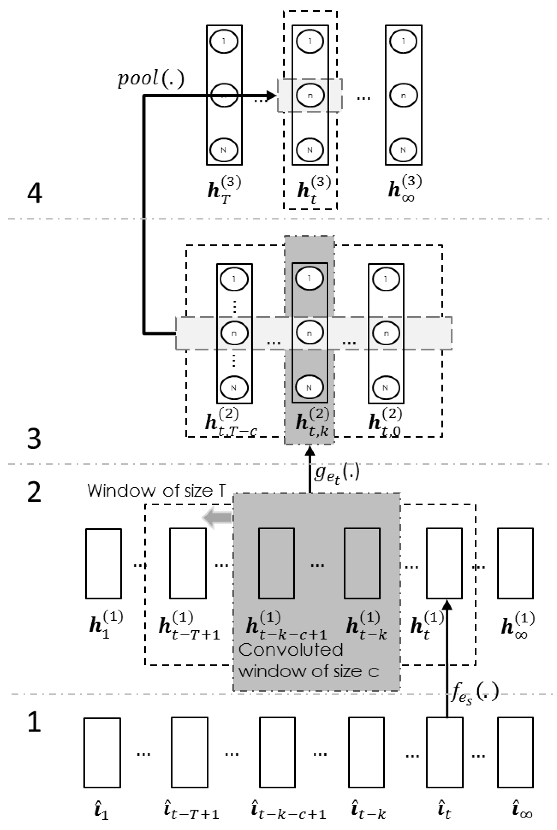
The proposed encoder model (Figure 5) has four layers. The first layer is the input layer, and the data are a list of unit upper-limb vectors $\widehat{\mathit{i}}$ from (27). Next, the second layer is the spatial transformation layer, which is optional. It transforms the data of the joints $\widehat{\mathit{i}}$ into the distributed spatial data:

$$\begin{array}{c}\hfill {\mathit{h}}^{\left(1\right)}=f_{e_s}(\widehat{\mathit{i}};{\mathit{\theta }}_{e_s})={\mathit{W}}_{e_s}·\widehat{\mathit{i}}+{\mathit{b}}_{e_s},\end{array}$$

(1)

where ${\mathit{\theta }}_{e_s}=\{{\mathit{W}}_{e_s}\in {\mathbb{R}}^{N^{\left(1\right)}\times 18},{\mathit{b}}_{e_s}\in {\mathbb{R}}^{N^{\left(1\right)}}\}$ are the model parameters, which were trained using contrastive divergence [19], and $N^{\left(1\right)}$ is the number of feature maps in the second layer. The third layer is the convolution layer. Initially, this layer pulls out a T sequence of spatial data ${\mathit{h}}_{(t-T+1):t}^{\left(1\right)}$. Sequentially, it pulls out a subset of c size from the above sequence for every k step, and k ranges from $0,\dots ,T-c$. In each k step, the model calculates the convoluted output:

$$\begin{array}{cc}{\mathit{h}}_{t,k}^{\left(2\right)}\hfill & =g_{e_t}({\mathit{h}}_{(t-k-c+1):(t-k)}^{\left(1\right)};{\mathit{\theta }}_{e_t})\hfill \\ & =\sigma ({\mathit{W}}_{e_t}·{\mathit{h}}_{(t-k-c+1):(t-k)}^{\left(1\right)}+{\mathit{b}}_{e_t}),\hfill \end{array}$$

(2)

where ${\mathit{\theta }}_{e_t}=\{{\mathit{W}}_{e_t}\in {\mathbb{R}}^{N^{\left(2\right)}\times c{N}^{\left(1\right)}},{\mathit{b}}_{e_t}\in {\mathbb{R}}^{N^{\left(2\right)}}\}$ are the parameters, which were also trained using contrastive divergence [19], and $\sigma \left(z\right)=\max (0,z)$ is a rectified function [20]. The last layer is the element-wise pooling layer. This layer merges the sequence from the previous layer $h_{t,0:(T-c)}^{\left(2\right)}$ to form:

$$\begin{array}{c}\hfill {\mathit{h}}_t^{\left(3\right)}=\mathrm{pool}\left({\mathit{h}}_{t,0:(T-c)}^{\left(2\right)}\right),\end{array}$$

(3)

where the $\mathrm{pool}\left(\right)$ can either be the $\mathrm{mean}$ or max operation. To simplify the encoding process from (1) to (3), the encoder function is reduced to:

$$\begin{array}{c}\hfill {\mathit{z}}_t={\mathit{h}}_t^{\left(3\right)}=f_e({\widehat{\mathit{i}}}_{(t-T+1):t};{\mathit{\theta }}_{e_s},{\mathit{\theta }}_{e_t}).\end{array}$$

(4)

Once the encoder can transform the input signal into the new vector/gesture space, the next step is to find a decoder to extrapolate the future joint states ${\widehat{\mathit{i}}}_{\left(t\right):(t+*)}^{\prime }$ given the boundary condition ${\widehat{\mathit{i}}}_{(t-p):(t-1)}$ and the encoded data ${\mathit{z}}_t$.

3.3. Model for Decoder

3.3.1. Long Short-Term Memory for Decoding

The aim of this section is to find a suitable recurrent neural network for the gesture modality. Many models, such as the temporal RBM (TRBM) [21], factored conditional RBM (FCRBM) [22], long short-term memory (LSTM) [23,24] and echo state network (ESN) [25], have been proven to generate various signals, such as motion, voice and handwriting. One of our preliminary experiments has shown that LSTM performed better for our case.

As a result, the proposed decoder architecture has four layers (Figure 6), and they are the input layer, LSTM layer, output layer and normalization layer. The input layer only assembles the necessary information for each iteration, that is:

$$\begin{array}{c}\hfill {\mathit{x}}_{i,t}={\left[\begin{array}{ccc}{\widehat{\mathit{i}}}_{(t-p):(t-1)}& {\mathit{z}}_t& {\tilde{\mathit{y}}}_{i,t-1}\end{array}\right]}^T,\end{array}$$

(5)

where ${\widehat{\mathit{i}}}_{(t-p):(t-1)}$ is the p number of previous upper-limb states, ${\mathit{z}}_t$ is the gesture style either from the encoder using (4) or the associator using (24), ${\tilde{\mathit{y}}}_{i,t-1}=({\mathit{y}}_{cell,t-1},\dots )$ is the previous LSTM states and $i\in \{in,g_{in},g_{for},g_{out}\}$.

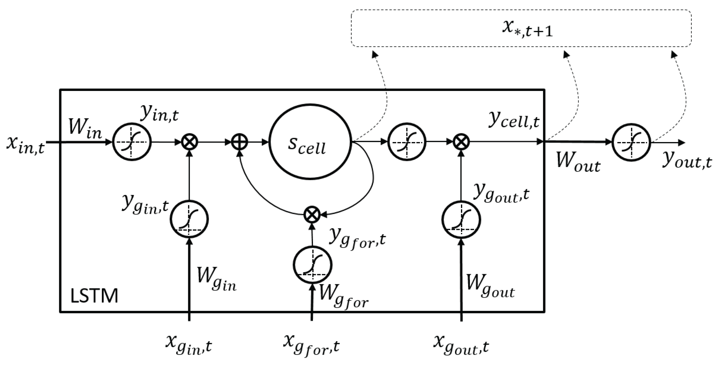
The second layer is the LSTM layer (Figure 7). It has many activation channels, like the input, gates, internal states and cell output. Each activation channel has two parameters: ${\mathit{W}}_i\in {\mathbb{R}}^{N^{gate}\times N^{\left(i\right)}}$ and ${\mathit{b}}_i\in {\mathbb{R}}^{N^{gate}}$, where $N^{gate}$ is the size of the cell. The following will describe the computation sequence. First of all, it concurrently computes the activation for the input and all of the gates. The activation for the input is:

$$\begin{array}{c}\hfill {\mathit{y}}_{in,t}={\sigma }_{[-{\alpha }_{in},{\alpha }_{in}]}({\mathit{W}}_{in}·{\mathit{x}}_{in,t}+{\mathit{b}}_{in}),\end{array}$$

(6)

while the activation for the gates is:

$$\begin{array}{c}\hfill {\mathit{y}}_{i,t}={\sigma }_{[0,1]}({\mathit{W}}_i·{\mathit{x}}_{i,t}+{\mathit{b}}_i),\end{array}$$

(7)

where ${\sigma }_{[a,b]}\left(z\right)=a+[(b-a)/(1+e^{-z})]$ is a modified generalized logistic function ranging from $[a,b]$ and $i\in \{g_{in},g_{for},g_{out}\}$. Next, it computes the activation for the internal state:

$$\begin{array}{c}\hfill {\mathit{s}}_{cell,t}={\mathit{y}}_{in,t}\circ {\mathit{y}}_{g_{in},t}+{\mathit{y}}_{g_{for},t}\circ {\mathit{s}}_{cell,t-1}.\end{array}$$

(8)

Lastly, it calculates the output cell:

$$\begin{array}{c}\hfill {\mathit{y}}_{cell,t}={\mathit{y}}_{g_{out},t}\circ {\sigma }_{[-{\alpha }_{cell},{\alpha }_{cell}]}\left({\mathit{s}}_{cell,t}\right).\end{array}$$

(9)

After completing the LSTM layer, the third layer transforms the cell output ${\mathit{y}}_{cell,t}$ into an instant of the joint state:

$$\begin{array}{c}\hfill {\mathit{y}}_{out,t}={\sigma }_{[-{\alpha }_{out},{\alpha }_{out}]}({\mathit{W}}_{out}·{\mathit{y}}_{cell,t}+{\mathit{b}}_{out}).\end{array}$$

(10)

Finally, the last layer is a series of normalization processes so that the inferred joint state ${\mathit{y}}_{out,t}$ is equivalent to the constrained joint state ${\widehat{\mathit{i}}}_t^{\prime }$. The following steps are the breakdown of the normalization processes. First of all, it denormalizes the inferred joint state ${\mathit{y}}_{out,t}$ to the concatenated unit vectors:

$$\begin{array}{c}\hfill \grave{\mathit{i}}=\mathbf{\sigma }{\mathit{y}}_{out,t}+\overline{\mathit{i}},\end{array}$$

(11)

where $\overline{\mathit{i}}$ is the mean of the data and $\mathbf{\sigma }$ is the standard deviation of the data. Because the constraints from (26) are valid, the second step repeats the same process:

$$\begin{array}{c}\hfill {\mathit{i}}_t^{\prime }={\left[\begin{array}{ccc}\frac{{\grave{\mathit{i}}}_{1:3}^T}{\parallel {\grave{\mathit{i}}}_{1:3}\parallel }& \cdots & \frac{{\grave{\mathit{i}}}_{16:18}^T}{\parallel {\grave{\mathit{i}}}_{16:18}\parallel }\end{array}\right]}^T.\end{array}$$

(12)

The above process ensures that the upper-limb orientations are indeed the concatenated unit vectors. Finally, it scales the concatenated unit vectors ${\mathit{i}}_t^{\prime }$ back to the normalized joint state ${\widehat{\mathit{i}}}_t^{\prime }$ using (27). The input layer from the next time step will then receive this result as one of its data. For simplification, the whole process from (5) to (12) is shortened to a decoder function:

$$\begin{array}{c}\hfill {\widehat{\mathit{i}}}_t^{\prime }=f_d({\widehat{\mathit{i}}}_{(t-p):(t-1)}^{\prime },{\mathit{z}}_t;{\mathit{\theta }}_d),\end{array}$$

(13)

where p is the number of previous state, ${\mathit{z}}_t$ is the encoded data either from (4) or (24) and ${\mathit{\theta }}_d$ is the optimized parameters for the model.

In conclusion, the decoder can extrapolate the future joint states ${\widehat{\mathit{i}}}_{\left(t\right):(t+*)}^{\prime }$ given the boundary condition ${\widehat{\mathit{i}}}_{(t-p):(t-1)}$ and the encoded data ${\mathit{z}}_t$. However, the decoder, alone, cannot produce an expressive collision-free gesture. Instead, it must work with a searching algorithm to find suitable encoded data ${\mathit{z}}_t^{\prime }$ that create collision-free motion.

3.3.2. Evolutionary Algorithm for Collision Avoidance

In this paper, the PLBM has an evolutionary algorithm (EA) to find a good candidate in the collision avoidance scenario, and there are three steps in this algorithm.

During initialization, the algorithm generates a pool of candidates ${\mathit{Z}}_1^{\left(o\right)}={\{{\mathit{z}}_1^{\left(o\right)},\dots ,{\mathit{z}}_M^{\left(o\right)}\}}_1$. This process involves mutation and crossover from a sample ${\mathit{Z}}_1^{\left(x\right)}=\{{\mathit{z}}_t,{\mathit{z}}_{t-1}^{\prime },\dots ,{\mathit{z}}_{t-p}^{\prime }\}$, where ${\mathit{z}}_t$ is the original encoded data and ${\mathit{z}}_{t-*}^{\prime }$ are the winning data from the previous time steps. In mutation, it randomly selects a specimen from the sample ${\mathit{z}}_i^{\left(x\right)}\in {\mathit{Z}}_1^{\left(x\right)}$ to reproduce a new candidate:

$$\begin{array}{c}\hfill {\mathit{z}}^{\left(o\right)}\sim \mathcal{N}({\mathit{z}}_i^{\left(x\right)},\sigma ),\end{array}$$

(14)

where $\sigma$ is a constant variance of a Gaussian distribution. On the other hand, the crossover randomly selects two specimens ${\mathit{z}}_i^{\left(x\right)}$ and ${\mathit{z}}_j^{\left(x\right)}$ to spawn a new candidate:

$$\begin{array}{c}\hfill {\mathit{z}}^{\left(o\right)}=\mathit{m}\circ {\mathit{z}}_i^{\left(x\right)}+\neg \mathit{m}\circ {\mathit{z}}_j^{\left(x\right)},\end{array}$$

(15)

where $\mathit{m}\in [\mathbf{0},\mathbf{1}]$ is a binary mask with a 0.5 mixing ratio. Once it has populated a pool of candidates ${\mathit{Z}}_1^{\left(o\right)}$, the second step is to evaluate all of them and select a list of them.

The evaluation process computes the score for each candidate, and the selection process picks a few of them for the next iteration. Firstly, the evaluation process computes the cost of each candidate with this fitness function:

$$\begin{array}{c}\hfill F_i=S\left(f_d\left({\mathit{z}}_i^{\left(o\right)}\right),f_d\left({\mathit{z}}_t\right)\right)+C\left(f_d\left({\mathit{z}}_i^{\left(o\right)}\right)\right),\end{array}$$

(16)

where $S(\mathit{X},\mathit{Y})\in \mathbb{R}$ measures the degree of similarity between $\mathit{X}$ and $\mathit{Y}$ and $C\left(\mathit{X}\right)\in \mathbb{R}$ counts the numbers of points outside the boundary. The $f_d\left({\mathit{z}}_i^{\left(o\right)}\right)$ is the decoded signals from the candidate ${\mathit{z}}_i^{\left(o\right)}$ over a time span, and $f_d\left({\mathit{z}}_t\right)$ is the decoded signals from the original encoded data ${\mathit{z}}_t$. Next, the selection process chooses a subset of the candidates ${\mathit{Z}}_1^{\left(w\right)}\subset {\mathit{Z}}_1^{\left(o\right)}$ with the lowest F score. Lastly, the algorithm will end if there $\exists i$ such that $F_i<\gamma$, where $\gamma$ is a predefined threshold; or else, the algorithm will go to the third step.

The third step repeats 1 and 2 until it finds a good candidate. Similar to the first step, the algorithm generates a pool of candidates at each iteration. In the k-th iteration, the sample ${\mathit{Z}}_k^{\left(x\right)}$ for populating the candidates is the selected candidates ${\mathit{Z}}_{k-1}^{\left(w\right)}$ from the previous iteration. The next step is the evaluation and selection processes. In the end, the cycle will only terminate when there $\exists i$ such that $F_i<\gamma$ or the loop has reached the maximum iteration.

In summary, the PLBM with EA can deliberately generate a collision-free motion that has a minimum distortion. In the next section, we present the last module, the associator, which can solve the decoupling problem.

3.4. Model for Associator

The associator is a modified multi-channel adaptive resonance associative map (ARAM) [26], which is an extension of the adaptive resonance theory (ART) model [27]. In the PLBM, the channels of the associator are the encoded nonverbal cues from the operator and the audiences. Ideally, the associator forms rules across the different channels for future querying. For better illustration, the following paragraphs will explain the learning and recalling process using three features, and they are the user’s face feature, the audience’s face feature and the user’s gesture feature.

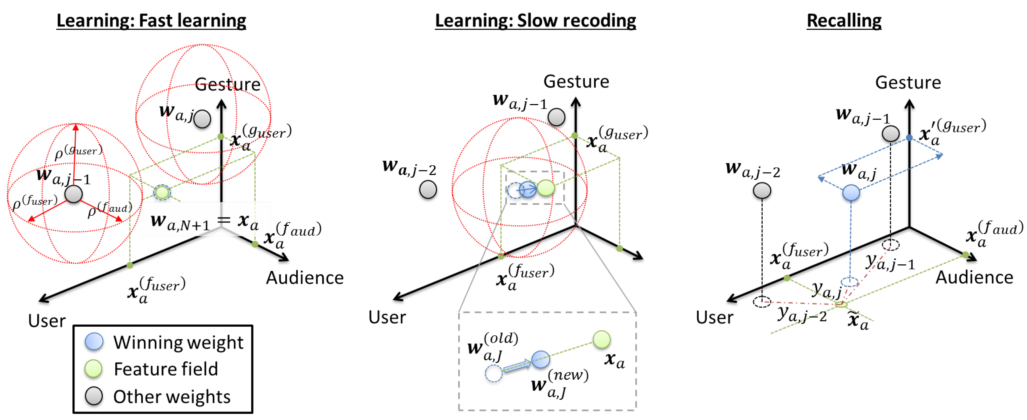
The learning process has four steps. The function for each step is: (1) preparing the input; (2) computing the choice activation; (3) finding the best activation; and (4) updating the weight through fast or slow learning. The first step only assembles the input features. Some existing ART models [28] have its input ${\mathit{x}}_a$ ranging within $[\mathbf{0},\mathbf{1}]$, but our approach intrinsically restricts the range by using the encoder. As a result, the input is:

$$\begin{array}{cc}{\mathit{x}}_a\hfill & ={\left[\begin{array}{ccc}{\mathit{x}}_a^{\left(f_{user}\right)}& {\mathit{x}}_a^{\left(f_{aud}\right)}& {\mathit{x}}_a^{\left(g_{user}\right)}\end{array}\right]}^T\hfill \\ & ={\left[\begin{array}{ccc}{\mathit{z}}_t^{\left(f_{user}\right)}& {\mathit{z}}_t^{\left(f_{aud}\right)}& {\mathit{z}}_t^{\left(g_{user}\right)}\end{array}\right]}^T,\hfill \end{array}$$

(17)

where ${\mathit{z}}_t^{\left(f_{user}\right)}$, ${\mathit{z}}_t^{\left(f_{aud}\right)}$ and ${\mathit{z}}_t^{\left(g_{user}\right)}$ are the encoded data of the user’s face feature, the audience’s face feature and the user’s gesture feature, respectively. Because the encoded data have no precise limit, there is also no known upper limit to the distance between two data. Therefore, we proposed a new choice activation function:

$$\begin{array}{c}\hfill y_{a,j}^k=\exp \left[-\sqrt{\frac{1}{M^k}{\Sigma }_{i=1}^{M^k}{(x_{a,i}^k-w_{a,ij}^k)}^2}\right],\end{array}$$

(18)

where $y_{a,j}^k\in [0,1]$ is the closeness index between input ${\mathit{x}}_a^k$ and weight ${\mathit{w}}_a^k$, $w_{a,ij}^k$ is the i-th element in the j-th node of the k-th channel, $M^k$ is the number of elements in the k-th channel and $k\in \{f_{user},f_{aud},g_{user}\}$. The third step finds the best activation index J. This process considers the results from all of the channels by:

$$\begin{array}{c}\hfill J=\underset{j}{\mathrm{argmin}}\left(\prod _{k\in \{f_{user},f_{aud},g_{user}\}}{y}_{a,j}^k\right).\end{array}$$

(19)

Lastly, there are two update methods, and they are known as the fast learner and slow recoder (Figure 8). The associator executes the faster learner:

$$\begin{array}{c}\hfill {\mathit{w}}_{a,N+1}={\mathit{x}}_a\end{array}$$

(20)

if $\forall j$ there $\exists k$ such that $y_{a,j}^k\le {\rho }^k$, where ${\rho }^k$ is the vigilance threshold of the k-th channel. On the other hand, if there $\exists j$ such that $\forall k$ satisfy $y_{a,j}^k\ge {\rho }^k$, then the slow recoding function updates the winner node ${\mathit{w}}_{a,J}$ by:

$$\begin{array}{c}\hfill {\mathit{w}}_{a,J}^{\left(new\right)}:=(1-\eta \left({\phi }_J\right))·{\mathit{w}}_{a,J}^{\left(old\right)}+\eta \left({\phi }_J\right)·{\mathit{x}}_a,\end{array}$$

(21)

where $\eta \left({\phi }_J\right)={({\phi }_J+1)}^{-1}$ is an adaptive learning rate, which decreases as the weight occurrence ${\phi }_J$ increases. In short, the associator will regularly create or update the relationships among all of the modalities. This process will come to a pause when there is a need to recall or replace one of the modalities.

The associator will switch to the recall mode (Figure 8) when there is one or more missing modalities. For this case, the following explanation assumes that the user’s gesture feature ${\mathit{z}}_t^{\left(g_{user}\right)}$ is missing. Hence, there is a newer and shorter input:

$$\begin{array}{c}\hfill {\mathit{x}}_a={\left[\begin{array}{ccc}{\mathit{x}}_a^{\left(f_{user}\right)}& {\mathit{x}}_a^{\left(f_{aud}\right)}& \varnothing \end{array}\right]}^T.\end{array}$$

(22)

During the initialization, the associator discards any weight ${\mathit{w}}_{a,j}$ if its frequency ${\phi }_j<\tau$, where $\tau$ is the pruning threshold. Next, the associator computes the choice activation using (18) on the observable feature fields ${\mathit{x}}_a^{\left(f_{user}\right)}$ and ${\mathit{x}}_a^{\left(f_{aud}\right)}$. It then finds the best activation:

$$\begin{array}{c}\hfill J=\underset{j}{\mathrm{argmax}}\left(\prod _{k\in \{f_{user},f_{aud}\}}{y}_{a,j}^k\right).\end{array}$$

(23)

From the best weight ${\mathit{w}}_{a,J}={\left[\begin{array}{ccc}{\mathit{w}}_{a,J}^{\left(f_{user}\right)}& {\mathit{w}}_{a,J}^{\left(f_{aud}\right)}& {\mathit{w}}_{a,J}^{\left(g_{user}\right)}\end{array}\right]}^T$, the associator can infer the gesture style:

$$\begin{array}{c}\hfill {\mathit{z}}_t^{\prime }={{\mathit{x}}_t^{\prime }}^{\left(g_{user}\right)}\approx {\mathit{w}}_{a,j}^{\left(g_{user}\right)}.\end{array}$$

(24)

The last process decodes the encoded data ${\mathit{z}}_t^{\prime }$ using the decoder function $f_d\left(\right)$ from (13) to estimate next joint state:

$$\begin{array}{c}\hfill {{\widehat{\mathit{i}}}^{\prime }}_t=f_d({\widehat{\mathit{i}}}_{(t-p):(t-1)}^{\prime },{\mathit{z}}_t^{\prime }),\end{array}$$

(25)

where ${\widehat{\mathit{i}}}_{(t-p):(t-1)}^{\prime }$ is the p number of previous upper-limb states. As a whole, this recalling strategy can retrieve associated data given a partial context.

In theory, the proposed framework can handle the teleoperating issues using its three components, and they are the encoders, decoders and associator. The next section will discuss the processes applied to the data to train each component.

3.5. Data and Its Preprocesses

The encoder and decoder should be trained with a diversified dataset because the diversified dataset can produce a generalized predictor. Therefore, the proposed gesture dataset is a combination of three datasets. The first source is the Microsoft action gesture [29]. It has three sets of 12 gaming gestures from ten people. However, only nine out of the 12 gestures were selected because they have more expressive upper-limb motion. The second source is the 3D iconic gesture dataset [30]. These gestures are speech-dependent, and the speech-dependent gesture is useful for our application. Furthermore, this dataset covers 29 subjects gesturing 20 different virtual objects. The last dataset is an in-house dataset, and it consists of deictic gestures and a few speech-dependent gestures (refer to Supplementary Material 4 for the description). It was noticed that all of the gesture styles in [29,30] are periodic gestures. Hence, a set of nonperiodic gestures, which are primary deictic gestures, were acquired and stored in the in-house dataset. In addition, the action and the iconic gestures are very intensive and dynamic. As a result, the in-house data also have waving and beating gestures, for which only a few of the joints are moving. Lastly, the combined dataset underwent a mirroring operation to double up the number of training data to 268,296, where each datum has five frames of poses. In conclusion, the final dataset has a high variety of gestures, and the next process is to normalize the data.

There is a series of processes to normalize the skeleton data. The first operation normalizes pose data so that the poses $\mathit{P}=\{{\mathit{p}}_1,\dots ,{\mathit{p}}_{20}\}\in {\mathbb{R}}^{3\times 20}$ are independent of the torso’s movement. Subsequently, the second process computes the upper-limb orientations:

$$\begin{array}{c}\hfill \mathit{i}={\left[\begin{array}{ccc}{\widehat{\mathit{o}}}_1& \dots & {\widehat{\mathit{o}}}_6\end{array}\right]}^T,\end{array}$$

(26)

where ${\widehat{\mathit{o}}}_j={\mathit{o}}_j/\parallel {\mathit{o}}_j\parallel$ is the relatively unit vector. The relative vector is ${\mathit{o}}_j={\mathit{p}}_{n_{j+1}}-{\mathit{p}}_{n_j}$, where $n=(5,6,7,9,10,11)$ is a list of poses from the skeleton data. The last operation is feature-rescaling, also known as standardization. Standardization scales all of the features, so that they are zero-mean and unit variance. As a result, the normalized data are:

$$\begin{array}{c}\hfill \widehat{\mathit{i}}=\frac{\mathit{i}-\overline{\mathit{i}}}{\mathbf{\sigma }},\end{array}$$

(27)

where $\overline{\mathit{i}}$ is the mean of the gesture data and $\mathbf{\sigma }$ is the standard deviation of the gesture data. Up to this point, the encoder can be trained using the normalized dataset, but more steps are required to train a decoder.

For training a decoder, there are two additional processes. The first process transforms the gesture signal into their gesture style ${\mathit{z}}_t$ using the encoder function at (4). Subsequently, the encoded data ${\mathit{z}}_t$ go through the standardization process. The second step then aligns the encoded data ${\mathit{z}}_t$ with the corresponding normalized data ${\widehat{\mathit{i}}}_{(t-T+1):t}$. In this paper, the encoded data ${\mathit{z}}_t$ have $T=25$ frames (5 FPS) of information, and the number of previous data is $p=5$. As a result, the initial condition is ${\widehat{\mathit{i}}}_{(t-T+1):(t-T+p)}$. During training, the decoder will generate the remaining $T-p=20$ frames, which is ${\widehat{\mathit{i}}}_{(t-T+p+1):t}$. In short, the encoding and alignment processes are the two addition steps for training a decoder. The next step is to add other modalities so that the associator can be trained and evaluated.

For the associator, there are two simulated datasets. Both the simulated datasets have three channels, and they are the operator’s facial channel, the audience’s facial channel and the operator’s gesture channel. The facial channels acquired their facial data from a facial expression dataset, the CK+dataset [31], while the gesture channel obtained its data from the above gesture dataset. The first set of data, the identity dataset (Figure 9, left), simulates a situation where an operator is talking to three different characters in a row. In each sequence, the operator and the audiences only display the neutral facial expression, but the operator motions different gesture styles towards each audience. In the second set, the expression dataset (Figure 9, right) simulates the operator talking to the same person. Each sequence has four parts, and each part has a unique gesture style. In terms of facial expression, the first part has the operator and audience making a neutral expression. The second and third have one of them displaying an arbitrary expression, while the others stay neutral. The last covers both expressing a random expression. In short, these two simulated datasets have three modalities so that we can observe the learning and recall process in the associator. With the availability of data for each component, the next section will present the evaluation criterion for training and evaluating the system.

3.6. Training and Evaluation Criteria

First of all, the objective function to evaluate the temporal parameters ${\mathit{\theta }}_{e_t}$ for the encoder is:

$$\begin{array}{c}\hfill {\mathit{\theta }}_{e_t}=\underset{{\mathit{\theta }}_{e_t}}{\mathrm{argmin}}\left(\frac{e\left({\mathit{\theta }}_{e_t}\right)}{d\left({\mathit{\theta }}_{e_t}\right)}+S({\mathit{h}}_{1:c}^{\prime \left(1\right)},{\mathit{h}}_{(t-c+1):t}^{\left(1\right)})+\zeta \left({\mathit{h}}_t^{\left(3\right)}\right)\right).\end{array}$$

(28)

The first item in the function is the ratio between intra-distance $e\left({\mathit{\theta }}_{e_t}\right)$ to inter-distance $d\left({\mathit{\theta }}_{e_t}\right)$. It describes the cluster distributions within the new vector space. The intra-distance $e\left({\mathit{\theta }}_{e_t}\right)$ measures the distance from all of the data to the cluster center within the same style, while the inter-distance $d\left({\mathit{\theta }}_{e_t}\right)$ measures the distance between the cluster centers of different styles. Next, the similarity function $S(\mathit{X},\mathit{Y})$ measures the error between $\mathit{X}$ and $\mathit{Y}$, where ${\mathit{h}}_{1:c}^{\prime \left(1\right)}=g_{e_t}^{-1}({\mathit{h}}_t^{\left(2\right)};{\mathit{\theta }}_{e_t})$ is the reconstruction of ${\mathit{h}}_{(t-c+1):t}^{\left(1\right)}$. Lastly, the $\zeta \left(\right)$ is the sparsity function. It measures the number non-zero elements in the encoded data ${\mathit{h}}_t^{\left(3\right)}$, and this promotes a more biased model. In short, the above criteria generate a vector space where similar gesture styles are closer to one another. Furthermore, the encoder with the sparse and distributed parameters can also transform unknown data.

Secondly, the evaluation function for the parameters of the decoder ${\mathit{\theta }}_d$ is:

$$\begin{array}{c}\hfill {\mathit{\theta }}_d=\underset{{\mathit{\theta }}_d}{\mathrm{argmin}}\left(S({\widehat{\mathit{i}}}_{dtw}^{\prime },{\widehat{\mathit{i}}}_{(t-T+p+1):t})\right),\end{array}$$

(29)

where ${\widehat{\mathit{i}}}_{dtw}^{\prime }$ is the aligned decoded signals and ${\widehat{\mathit{i}}}_{(t-T+p+1):t}$ is the training signals. The following steps compute the aligned decoded signals ${\widehat{\mathit{i}}}_{dtw}^{\prime }$. The first step generates the decoded signal ${\widehat{\mathit{i}}}_{(t-T+p+1):t}^{\prime }$ using (13) and the encoded data ${\mathit{z}}_t$. The next process arranges the decoded signal ${\widehat{\mathit{i}}}_{(t-T+p+1):t}^{\prime }$ into the aligned decoded signals ${\widehat{\mathit{i}}}_{dtw}^{\prime }$ using the dynamic time warping (DTW) algorithm. Lastly, the similarity function measures the error between the aligned signals ${\widehat{\mathit{i}}}_{dtw}^{\prime }$ to the original signals ${\widehat{\mathit{i}}}_{(t-T+p+1):t}$. In conclusion, the goal is to find a suitable parameter ${\mathit{\theta }}_d$ for the decoder so that the decoder can generate the specific gesture signal given a gesture style.

For the associator, the objective primarily focuses on reconstructing the user’s gestures given the user’s and audiences’ facial features. Hence, the initial step learns the relationship between these modalities using (17) to (21). These operations compute the knowledge-based ${\mathit{W}}_a$, which is parameterized by ${\mathit{\theta }}_a=\{{\rho }^{\left(f_{user}\right)},{\rho }^{\left(f_{aud}\right)},{\rho }^{\left(g_{user}\right)}\}$. Subsequently, the associator retrieves the missing modalities, that is the encoded gesture ${\mathit{z}}_t^{\prime }$ using (22) to (24). Using (25), it generates the decoded signals ${\widehat{\mathit{i}}}_{(t+1):(t+T)}^{\prime }$, and it is aligned to form ${\widehat{\mathit{i}}}_{dtw}^{\prime }$. Similar to (29), the aim is to find the best parameters:

$$\begin{array}{c}\hfill {\mathit{\theta }}_a=\underset{{\mathit{\theta }}_a}{\mathrm{argmin}}\left(S({\widehat{\mathit{i}}}_{dtw}^{\prime },{\widehat{\mathit{i}}}_{(t+1):(t+T)})\right)\end{array}$$

(30)

that minimize the error between the aligned decoded signal ${\widehat{\mathit{i}}}_{dtw}^{\prime }$ and the original signal ${\widehat{\mathit{i}}}_{(t+1):(t+T)}$.

Besides evaluating the components, there are also functions to test the framework for the different scenarios. The first evaluation function measures the smoothness in a multivariate signal. The jerky index:

$$\begin{array}{c}\hfill J\left(\mathit{Y}\right)=\left(\sum _{t=1}^T\sum _{m=1}^M\frac{{\delta }^3{y}_{m,t}}{\delta t^3}\right)/\left(TM\right)\end{array}$$

(31)

is the average jerk measurement across a feature, where $y_{m,t}$ is the magnitude of the m feature at t time. The second evaluation function measures the total points outside the boundaries. The collision function is:

$$\begin{array}{c}\hfill C\left(\mathbf{A}\right)=\sum _{i\in \{x,y,z\}}(U\left(i\right)+L\left(i\right)),\end{array}$$

(32)

where $U\left(i\right)={\sum }_{m_i}{\sum }_{t=1}^T[a_{m_i,t}\ge u_i]$ and $L\left(i\right)={\sum }_{m_i}{\sum }_{t=1}^T[a_{m_i,t}\le l_i]$ are the total points outside the upper limit $u_i$ or lower limit $l_i$ at the i axis (Figure 10). The $m=\left({(1,4,\dots ,13,16)}_x,{({\left(\dots \right)}_x+1)}_y,{({\left(\dots \right)}_x+2)}_z\right)$ is the corresponding skeleton indexes with respect to the axis. Lastly, the similarity function $S(\mathit{X},\mathit{Y})$, which measures the accuracy between two signals, can also measure the degree of expressivity between the generated signal with respect to the original signal. In this paper, the similarity function $S(\mathit{X},\mathit{Y})$ is the mean square error function:

$$\begin{array}{c}\hfill \mathrm{MSE}(\mathit{X},\mathit{Y})=\left(\sum _t^T\sum _m^M{(x_{m,t}-y_{m,t})}^2\right)/\left(TM\right),\end{array}$$

(33)

where $\mathit{X},\mathit{Y}\in {\mathbb{R}}^{M\times T}$.

In summary, this section has presented a list of procedures and a list of evaluation functions to achieve the overall goals. The following section will show the different experiments and their results in term of these criteria.

4. Results

This section presents four experiments to show the effectiveness of the PLBM (refer to the links in Supplementary Material 3 for the video of the experiment. The first set of experiments demonstrates the fundamental functions of the encoder and decoder. The second experiment presents the associator ability to replace a missing modality during a decoupling scenario. Next, the third experiment compares the differences between the distributed spatiotemporal and the distributed spatial representation in various connection conditions. Finally, the last experiment investigates the differences between the deliberate and the reactive safety mechanism.

4.1. Encoding and Decoding Expressive Gesture

Figure 11a shows a set of spatiotemporal features. The figure on the left displays 30 of encoded features, where the x-axis is the relative time step, and the y-axis is the input variables. In the same figure, the brighter intensity indicates a stronger correlation between the variables at the given time step. On the right, the figure is the three-dimensional view of the fifth spatiotemporal feature. This figure displays a clearer glimpse of the intensity with respect to time. From this viewpoint, this feature is smooth with respect to time. In summary, the spatiotemporal features seem to capture the underlying structure of the signals, and the next paragraph will discuss the characteristics of the activation given different gesture styles.

Figure 11b shows the differences between the various output layers from a segment of gesture signals, which has two gesture styles. The following descriptions are the observations from each layer. For the input layer, the differences in the frequency and magnitude of the signals can separate the two gesture styles. In contrast, the two gestures, from $h^{\left(2\right)}$ and $h^{\left(3\right)}$, can be differentiated from the degree of the activation, alone. However, there is a delay in the transition, about 25 frames, in $h^{\left(3\right)}$ as compared to $h^{\left(1\right)}$ or $h^{\left(2\right)}$. In short, the encoder successfully maps the gesture signal into its style. In the next experiment, it will illustrate the generation power of the decoder given the gesture style.

Figure 11c displays nine decoded signals from nine distinctive gesture styles, and the descriptions below are the observations. Firstly, the dynamics of reconstructed gestures converges over time. All of the signals converge in less than 1/10 of the duration (100 time steps), which is about two seconds. Moreover, there is a smooth transition between two gesture styles, which is shown in the detailed skeleton view. Lastly, the model captures the contextual dynamics. For the decoder, the input is only the encoded data and previous states, yet the decoder can synthesize the nine distinct gestures without changing its parameters. In conclusion, the selected decoder model has shown promising results as it can reconstruct various gesture dynamics given the encoded information. In the next section, were will show the performance of the PLBM as a whole.

4.2. Coping with Decoupling Using the Associator

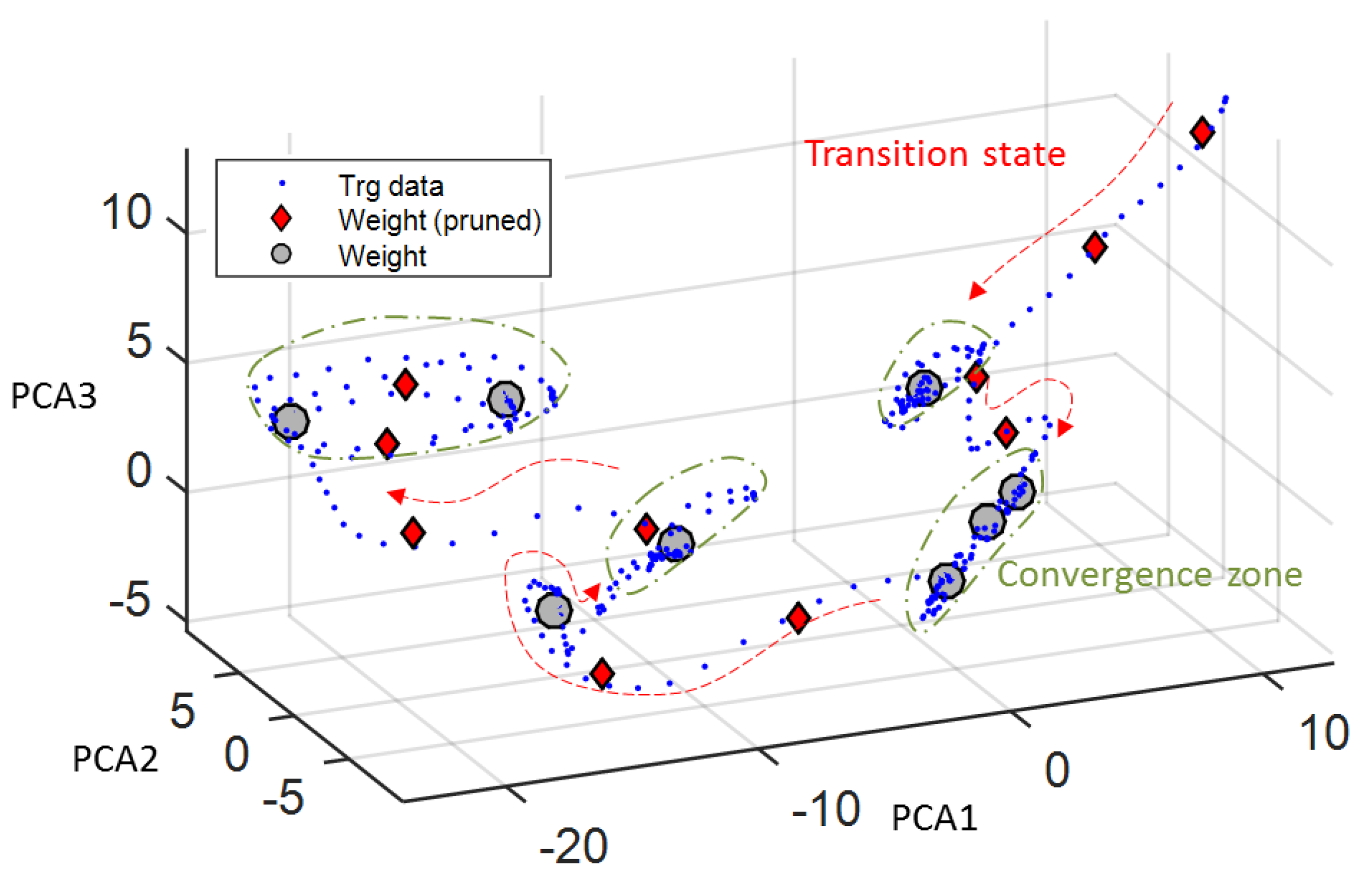
Figure 12 displays the output of the associator after the learning process given a sequence in the expression dataset (Figure 9). For the first observation, there are two possible states: convergence zone and transition state. The convergence zone is the region where the data are gathered, and there are four distinct zones in Figure 12. On the other hand, the transition state forms the trail leading from one cluster to the other. Secondly, the convergence zone holds more data as compared to the transition state. Given an interval of 100 frames at each state, most of the training data are in the convergence zone forming a region of interest. Finally, the associator has captured the region of interest, and there is only a small amount of the generated rules. For instance, the final weight size is 55.6% smaller than the initial size, not to mention, most of the final weights are in the convergence zone. Once the associator gathers all of its rules, the next step is to test the recall process.

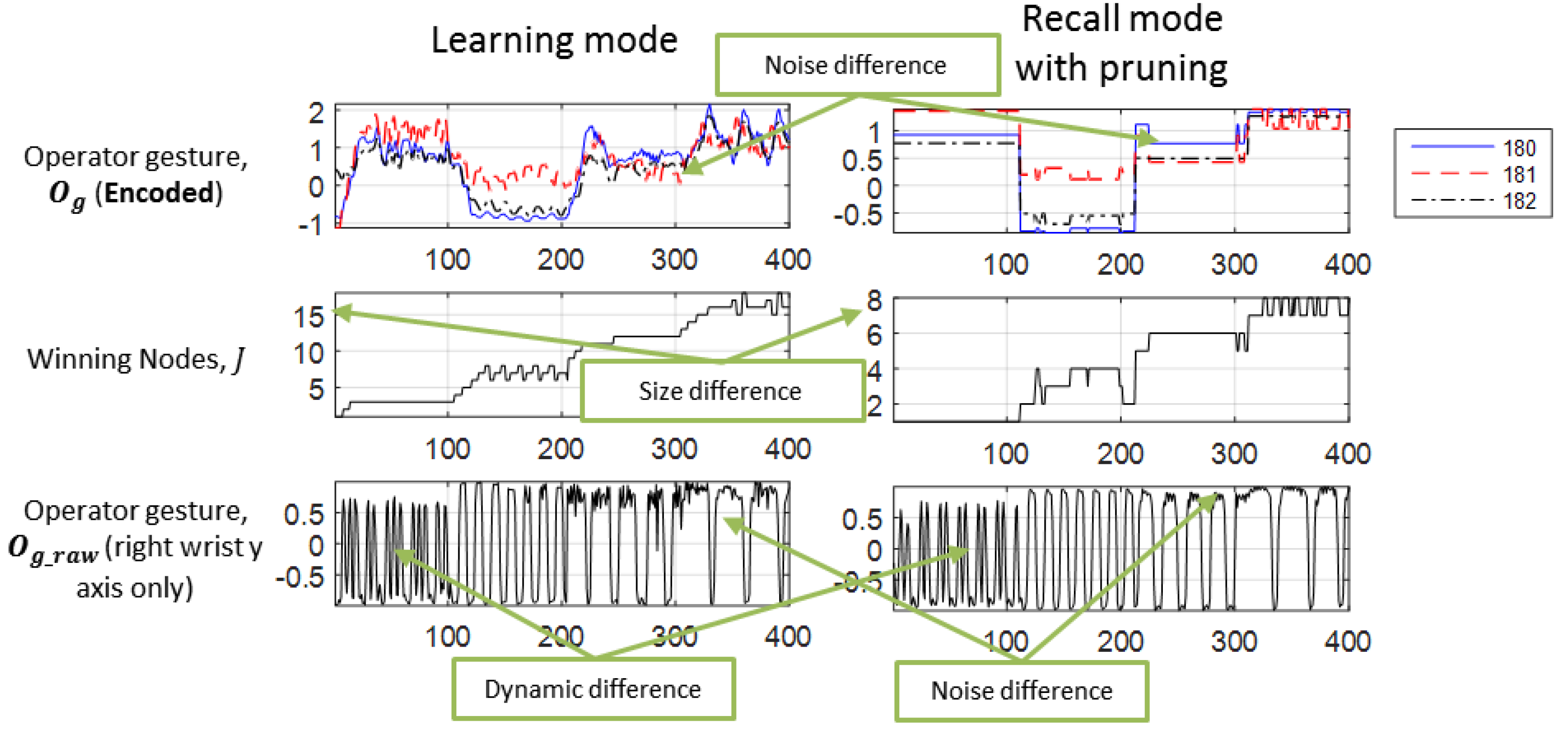
The following notes are the observations while we compared the synthesized gesture to the ground truth. From Figure 13, their dynamics are similar but not the same. The training gesture has mostly three peaks when the time step is <100, but the recalled gesture has only two peaks in all instances. Next, the synthesized signal is smoother than the training signal. Specifically, there is noise in the training gesture when the intensity is more than 0.5. Favorably, the recalled gesture displays less disturbance in that region. In brief, the PLBM with the associator can evoke a congruent and similar gesture given the facial features. The next section will look into the performance of the PLBM when there is a drop rate in the connection.

4.3. Reconstruction in an Unstable Connection

An inserting scenario is a situation when the network connection is unstable. Network congestion over a wireless network might result in packet loss. Retransmitting a lost packet is a solution, but it is not an optimal solution for teleoperating because it increases latency. A more optimal option is to adopt the no retransmission strategy to lower latency, which involves losing data. Thus, the remote system must find a valid motion when network congestion occurs. In this experiment, the gesture signal is randomly dropped using Bernoulli sampling at a probability of connection $P\left(connect\right)\in (0,1)$. The aim of the investigation is to analyze the effects of the connectivity on the accuracy and smoothness of the different signals.

In this experiment, we observed the characteristics of the signals from five different sources. The first signal is the training gesture (A). It came from the identity and expression dataset that has 15 sequences with three to four gesture styles each. The second signal is the fully-connected PLBM gesture (B). It is the decoded signal from the incoming encoded data when there is no dropout. The third signal is the decoded gesture using the recalled encoded data (C). Similar to Section 4.2, this method recovers the gesture style from the remaining modalities, which is the audience’s facial expression. The fourth signal is the synthesized gesture from the last received data (D). It just inserts the last received data because the encoder transmits styles and not poses. Finally, the last signal is the imitated gesture using last received pose (E). Unlike D, it only inserts the last received pose because the transmitted data have spatial information only.

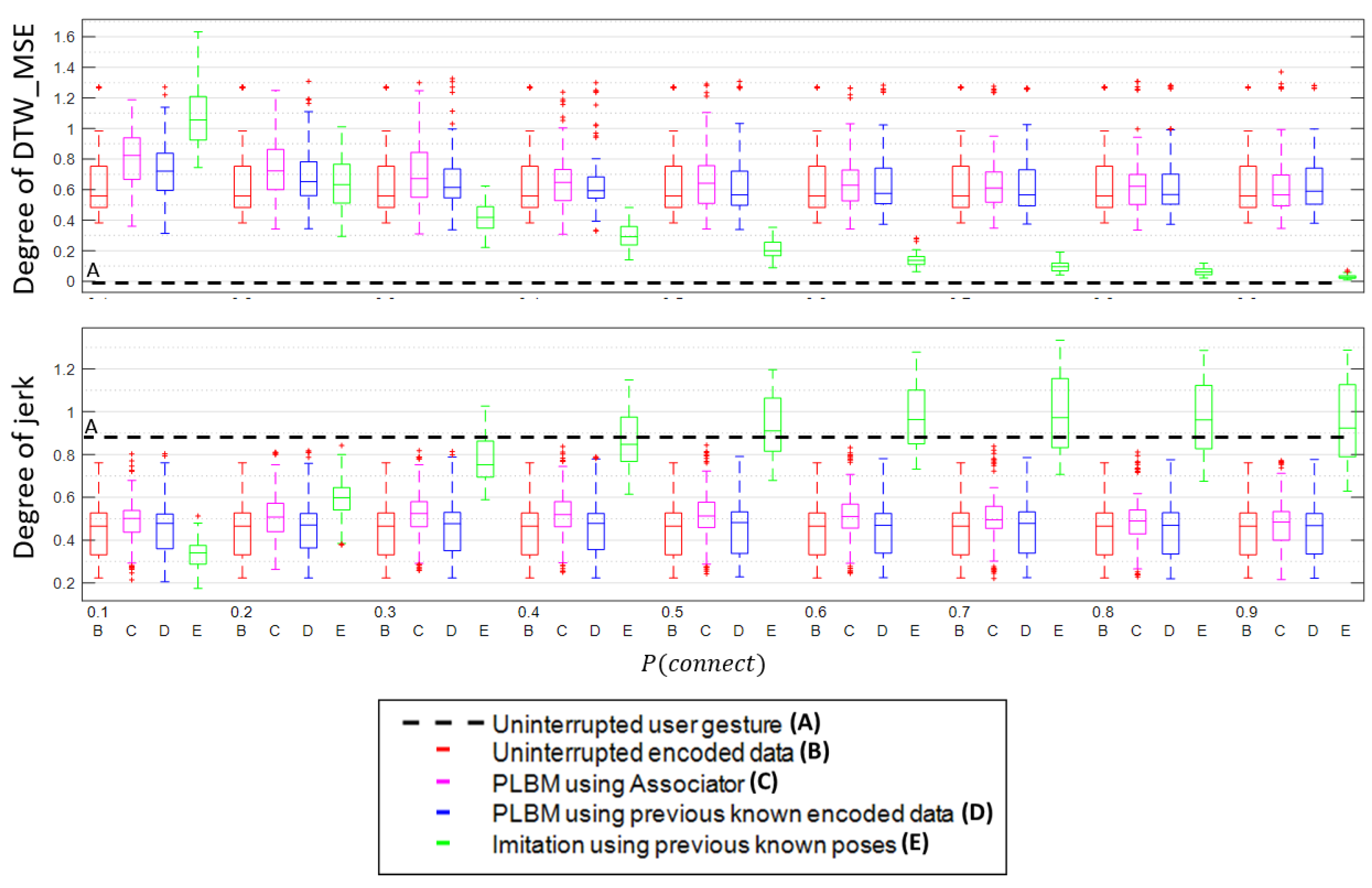
This section has two figures to demonstrate the effect of dropout on the different signals, and they are from the same experimental setup. Figure 14 shows a visual segment of the various signals when the rate of successful connection is 0.5. It provides a visual observation of the smoothness and accuracy between different signals. On the other hand, Figure 15 displays the statistical results across a wider range of connections. There is a total of 75 (15 × 5) sequences. Each of them has a unique connection sequence All of the plots, except for A, show the distribution of the results to demonstrate the consistency of each approach. In brief, both figures illustrate the outcome from the same experimental setup. One of them is a visual observation, while the other is the quantitative result.

Figure 15 shows the overall performance of the various signals across different degree of connection using both datasets from Figure 9. From the top figure, D is more accurate than C for most cases. D is closer to B when the connection is between 0.1 and 0.8. Eventually, D and C converge with B at 0.9. From the other figure, all of the PLBM signals (B, C and D) are smoother than the other two signals (A and E). On average, the PLBM signals have their jerk indexes between 0.45 and 0.50. On the contrary, A has its jerk index at 0.88, and E has most of its index above 0.6. Lastly, the jerk index for E is higher than A when the connection rate is high. The jerk index of E is above 0.88 when the connection is from 0.5 to 0.9.

In summary, the PLBM with the last known gesture style (D) has a better overall performance. It produces smoother synthesized signal than the other approaches, and the accuracy is similar to B, its uninterrupted counterpart. In the next section, we will look into the performance of the PLBM when there are boundary constraints.

4.4. Finding a Collision-Free Expressive Gesture

There are two approaches for this experiment, and they are the deliberative and reactive mechanism. The reactive mechanism replaces any out-of-bound point with its last received data, which have only spatial information. On the other hand, the deliberative method fits the synthesized motion into the boundary and preserves the expressiveness of the motion (Figure 16). The goal is to compare the difference between the reactive and deliberative mechanism in terms of accuracy and smoothness.

Figure 17 shows the comparison between the reactive and deliberative safety planner in terms of smoothness, accuracy and collision. The first observation is that the deliberative approach produces a smoother signal than the reactive approach. From Figure 17a, the deliberate approach, the PLBM with EA, has a degree of jerk near 0.516, while the reactive approach, the imitation with constraints, has a value of 0.917. Besides, the motion from PLBM with EA has a similar dynamics as the PLBM without constraint. Figure 17b shows that the deliberate approach has an accuracy of 0.726 compared to the PLBM without constraints, that is 0.559. Lastly, none of the generated points from PLBM with EA are out-of-bound. Figure 17c shows that neither the PLBM with EA nor imitation with constraints have their points outside the boundary. In short, the deliberate approach, the PLBM with EA, has a better overall performance. It synthesizes a smoother signal than the reactive approach. Even though the deliberative approach has a higher error rate than the reactive approach, its error rate is still similar to the PLBM without constraints.

5. Conclusions

In conclusion, the aim of the research was to study and develop a module that can solve the teleoperating issues in CATR. From the above experiment, the following items are the summaries of the PLBM achieving the objectives:

• For preserving expressiveness, the PLBM automatically encodes gestures into a distributed output. It can then extrapolate its future joint state using the distributed output, and the generated signal has similar dynamics to the training gesture.
• For minimizing the cognitive load, the PLBM has the natural interface to obtain the gesture. Furthermore, the PLBM uses automatic encoders, decoders and an associator for minimizing human intervene.
• If the operator’s hands are not free, the operator can delegate his/her gesturing modality to the PLBM with the associator.
• If the connection is not stable, the CATR can continue to gesticulate by generating the gesture using the last known gesture style.
• The PLBM can tune the incoming encoded data so that the decoded gesture is collision-free and has similar expressiveness.

However, the PLBM has a few limitations. Firstly, the completeness and correctness of the features depend on the training data. The current combined dataset only has three datasets, and these datasets might not cover all conversations. Secondly, the time consumption for the evolutionary algorithm to find a candidate to suit the environment is high and inconsistent. The current approach adopted the evolutionary algorithms, which might take a long time. In the worst case, the time needed might disrupt the flow of a conversation. The third limitation lies in the averaging component in the encoder model, which removes the phase information. Unfortunately, it produces a delay during the transition, and a significant delay might disrupt the flow of the conversation. In summary, the PLBM has its advantages, but also has a few limitations using the selected models. Thus, the existing PLBM model still requires plenty of studies and researches.

The below items are a list of future works to increase the complexity and realism of the dataset. The first item is to increase the diversity of the training data by integrating more dataset. It is beneficial to train the model from a diversified dataset because it improves generalization. Other work can focus on expanding the modalities because nonverbal signals cover a broad spectrum. For instance, there are other nonverbal cues like vocal cues, gaze and body posture. Some effort can be invested in getting a realistic dataset by employing a group of communication partners. The control group contains pairs of friends, and we can randomly match them to create various behaviors. In short, the objectives for the future works anchor the effort on increasing the realism of the dataset, so that we can better examine the framework.

References

1. Pang, W.C.; Wong, C.Y.; Seet, G. Design and development of edgar—A telepresence humanoid for robot-mediated communication and social applications. In Proceedings of the IEEE International Conference on Control and Robotics Engineering, Singapore, 2–4 April 2016; pp. 1–4. [Google Scholar]
2. Ekman, P. Emotional And Conversational Nonverbal Signals. In Language, Knowledge, and Representation; Springer: Dordrecht, The Netherlands, 2004; pp. 39–50. [Google Scholar]
3. Bavelas, J.; Chovil, N.; Coates, L. Gestures specialized for dialogue. Personal. Soc. Psychol. 1995, 21, 394–405. [Google Scholar] [CrossRef]
4. Neff, M.; Wang, Y.; Abbott, R.; Walker, M. Evaluating the Effect of Gesture and Language on Personality Perception in Conversational Agents. In Proceedings of the International Conference on Intelligent Virtual Agent, Philadelphia, PA, USA, 20–22 September 2010; pp. 222–235. [Google Scholar]
5. Adalgeirsson, S.O.; Breazeal, C. MeBot: A robotic platform for socially embodied telepresence. In Proceedings of the ACM/IEEE International Conference on Human-Robot Interaction, Osaka, Japan, 2–5 March 2010; pp. 15–22. [Google Scholar]
6. Kristoffersson, A.; Coradeschi, S.; Loutfi, A. A Review of Mobile Robotic Telepresence. Adv. Hum. Comput. Interact. 2013, 2013, 1–17. [Google Scholar] [CrossRef]
7. Park, H.; Kim, E.; Jang, S.; Park, S. HMM-based gesture recognition for robot control. In Proceedings of the Iberian Conference on Pattern Recognition and Image Analysis, Estoril, Portugal, 7–9 June 2005; pp. 607–614. [Google Scholar]
8. Lau, M.; Bar-Joseph, Z.; Kuffner, J. Modeling spatial and temporal variation in motion data. ACM Trans. Graph. 2009, 28, 171. [Google Scholar] [CrossRef]
9. Hinton, G.E. Connectionist learning procedures. Artif. Intell. 1989, 40, 185–234. [Google Scholar] [CrossRef]
10. Hasegawa, K.; Nakauchi, Y. Preliminary Evaluation of a Telepresence Robot Conveying Pre-motions for Avoiding Speech Collisions. In Proceedings of the Second International Conference on Human-Agent Interaction, Tsukuba, Japan, 29–31 October 2014; pp. 5–8. [Google Scholar]
11. Hartmann, B.; Mancini, M.; Pelachaud, C. Implementing expressive gesture synthesis for embodied conversational agents. In Proceedings of the 6th International Conference on Gesture in Human-Computer Interaction and Simulation, Berder Island, France, 18–20 May 2005; pp. 188–199. [Google Scholar]
12. Neff, M.; Kipp, M.; Albrecht, I.; Seidel, H. Gesture modeling and animation based on a probabilistic re-creation of speaker style. ACM Trans. Graph. 2008, 27. [Google Scholar] [CrossRef]
13. Taylor, G.W.; Hinton, G.E.; Roweis, S.T. Modeling human motion using binary latent variables. In Proceedings of the Advances in Neural Information Processing Systems, Vancouver, BC, Canada, 4–7 December 2006; pp. 1345–1352. [Google Scholar]
14. Xia, S.; Wang, C. Realtime Style Transfer for Unlabeled Heterogeneous Human Motion. ACM Trans. Graph. 2015, 34, 119. [Google Scholar] [CrossRef]
15. Danziger, K. Interpersonal Communication; Pergamon Press: Oxford, UK, 1976; p. 238. [Google Scholar]
16. Chartrand, T.L.; Bargh, J.A. The chameleon effect: The percpetion-behavior link and social interaction. J. Personal. Soc. Psychol. 1999, 76, 893–910. [Google Scholar] [CrossRef]
17. Hinton, G.E.; Osindero, S.; Teh, Y.W. A Fast Learning Algorithm for Deep Belief Nets. Neural Comput. 2006, 18, 1527–1554. [Google Scholar] [CrossRef] [PubMed]
18. Bengio, Y. Learning Deep Architectures for AI. Found. Trends Mach. Learn. 2009, 2, 1–127. [Google Scholar] [CrossRef]
19. Hinton, G.E. Training products of experts by minimizing contrastive divergence. Neural Comput. 2002, 14, 1771–1800. [Google Scholar] [CrossRef] [PubMed]
20. Nair, V.; Hinton, G.E. Rectified linear units improve restricted boltzmann machines. In Proceedings of the International Conference on Machine Learning, Haifa, Israel, 21–24 June 2010; pp. 807–814. [Google Scholar]
21. Sutskever, I.; Hinton, G.E. Learning multilevel distributed representations for high-dimensional sequences. In Proceedings of the International Conference on Artificial Intelligence and Statistics, San Juan, Puerto Rico, 21–24 March 2007; pp. 548–555. [Google Scholar]
22. Taylor, G.W.; Hinton, G.E.; Roweis, S.T. Two Distributed-State Models for Generating High-Dimensional Time Series. J. Mach. Learn. Res. 2011, 12, 1025–1068. [Google Scholar]
23. Hochreiter, S.; Schmidhuber, J. Long short-term memory. Neural Comput. 1997, 9, 1735–1780. [Google Scholar] [CrossRef] [PubMed]
24. Gers, F.A.; Schmidhuber, J.; Cummins, F. Learning to forget: Continual Prediction with LSTM. Neural Comput. 2000, 12, 2451–2471. [Google Scholar] [CrossRef] [PubMed]
25. Jaeger, H. A Tutorial on Training Recurrent Neural Networks, Covering BPPT, RTRL, EKF and the “Echo State Network” Approach; German National Research Center for Information Technology: St Augustin, Germany, 2002; pp. 1–48. [Google Scholar]
26. Tan, A.H.; Soon, H.S. Concept hierarchy memory model: A neural architecture for conceptual knowledge representation, learning, and commonsense reasoning. Int. J. Neural Syst. 1996, 7, 305–319. [Google Scholar] [CrossRef] [PubMed]
27. Carpenter, G.A.; Grossberg, S. ART 2: Self-organization of stable category recognition codes for analog input patterns. Appl. Opt. 1987, 26, 4919–4930. [Google Scholar] [CrossRef] [PubMed]
28. Frank, T.; Kraiss, K.F.; Kuhlen, T. Comparative analysis of fuzzy ART and ART-2A network clustering performance. IEEE Trans. Neural Netw. 1998, 9, 544–559. [Google Scholar] [CrossRef] [PubMed]
29. Fothergill, S.; Mentis, H.; Kohli, P.; Nowozin, S. Instructing people for training gestural interactive systems. In Proceedings of the SIGCHI Conference on Human Factors in Computing Systems, Austin, TX, USA, 5–10 May 2012; pp. 1737–1746. [Google Scholar]
30. Morency, L.P.; Sadeghipour, A. Available online: http://projects.ict.usc.edu/3dig/ (accessed on 28 January 2016).
31. Lucey, P.; Cohn, J.F.; Kanade, T.; Saragih, J.; Ambadar, Z.; Matthews, I.; Ave, F. The Extended Cohn-Kanade Dataset (CK+): A complete dataset for action unit and emotion-specified expression. In Proceedings of the IEEE Conference on Computer Vision and Pattern Recognition-Workshops, San Francisco, CA, USA, 13–18 June 2010; pp. 94–101. [Google Scholar]
Figure 1. The different mediums for interpersonal communication. (a) Various mediums for interpersonal communication ranging from FTFC to CMC; (b) an instance of a customizable anthropomorphic telepresence robot, EDGAR-1 (Expression Display & Gesturing Avatar Robot).
Robotics 06 00016 g001
Figure 2. The three possible teleoperating issues while operating a CATR using a natural interface.
Robotics 06 00016 g002
Figure 3. The perception-link behavior model. (a) Block diagram of the perception-link behavior model; (b) the perception-link behavior model in the CATR’s framework.
Robotics 06 00016 g003
Figure 4. The functions of each component in a PLBM.
Robotics 06 00016 g004
Figure 5. Four-layer encoder model. For the detailed description of the selection of this model and its parameters, please refer to Supplementary Material 2, Section 1.
Robotics 06 00016 g005
Figure 6. Decoder model with rollout with time.
Robotics 06 00016 g006
Figure 7. Forward pass of an LSTM cell with input, output and forget gates. For the detailed description of the selection of its parameters, please refer to Supplementary Material 2, Section 2.
Robotics 06 00016 g007
Figure 8. Learning and recalling processes in the associator module. For the detailed description of the selection of its parameters, please refer to Supplementary Material 2, Section 3.
Robotics 06 00016 g008
Figure 9. A sample data from the identity (left) and expression (right) dataset.
Robotics 06 00016 g009
Figure 10. The collection wrist positions in various views and the projected boundaries. (a) The top view: z vs. x. (b) The side view: y vs. z. (c) The front view: y vs. x.
Robotics 06 00016 g010
Figure 11. Visualization of features and results from the encoder and the decoder. (a) The 30 convolution features (left) and its fifth convolution feature (right) by CNN-RBMusing a 15-FPS dataset. (b) The encoded output given a segment of gesture with two different styles with specific features. (c) The LSTM internal states and output, nine gestures, given their encoded data.
Robotics 06 00016 g011
Figure 12. The results from learning using the associator module.
Robotics 06 00016 g012
Figure 13. The operator’s gesture signal and the reconstructed gesture signal.
Robotics 06 00016 g013
Figure 14. A segment of the gesture from different approaches when the success of connection is 0.5.
Robotics 06 00016 g014
Figure 15. The distribution (minimum, first quartile, median, third quartile, and maximum) of the quality for gestures with various connection rates from 0.1 to 0.9. It was conducted over 15 training sequences with five replicas.
Robotics 06 00016 g015
Figure 16. Motion points of the wrists with constraints in different spatial views. (a) The ground truth motion from the data set. (b) The motion generated using PLBM without constraint. (c) The motion generated using PLBM with EA and constraint.
Robotics 06 00016 g016
Figure 17. The distribution (minimum, first quartile, median, third quartile and maximum) of the evaluation criterion over 15 training sequences with five replicas given a fixed boundary. (a) The results corresponding to the amount of jerk. (b) The degree of accuracy with respect to the training motion. (c) The total number of collision points.
Robotics 06 00016 g017