Application of the Naive Bayes Classifier for Representation and Use of Heterogeneous and Incomplete Knowledge in Social Robotics

Abstract

As societies move towards integration of robots, it is important to study how robots can use their cognition in order to choose effectively their actions in a human environment, and possibly adapt to new contexts. When modelling these contextual data, it is common in social robotics to work with data extracted from human sciences such as sociology, anatomy, or anthropology. These heterogeneous data need to be efficiently used in order to make the robot adapt quickly its actions. In this paper we describe a methodology for the use of heterogeneous and incomplete knowledge, through an algorithm based on naive Bayes classifier. The model was successfully applied to two different experiments of human-robot interaction.

1. Introduction

In the near future, in order to be effectively integrated into human environments, robots should be able to interact using an adequate level of cognition. Such cognition should be flexible enough to allow the robots to understand human actions, store knowledge efficiently and react accordingly, taking into account changes in context.

Among artificial intelligence techniques and machine learning methods, a wide variety of techniques are effective under determined conditions. For example, neural networks can approximate non-linear functions, whereas reinforcement learning can effectively solve game playing and pathfinding problems. Unsupervised learning, on the contrary, has the advantage of not needing labelled data for a training set. However, depending on the specific problem, most of these techniques may be inefficient. In general, the "no free lunch" theorem applies to machine learning [1], as for each specific problem the most fitting technique is going to be different.

Robots should learn from experience and from interactions with other agents they encounter in their environment in a similar way as animals, including humans. From the point of view of learning algorithms, this setting imposes certain constraints which often do not hold for mainstream machine learning applications. Such constraints include finite storage and memory, and the need to learn incrementally, by modifying behavior after each or every few experiences. With such conditions, online learning is the natural approach for robots [2].

Adaptive robotics is a term that is used to indicate that the study of robots can exhibit an adaptive behavior to the environment. The concept is true for several applications.

While a great deal of machine learning research has focused on batch learning, which is more amenable to mathematical formalization [3], more recently, due to the increasing availability of very large datasets and continuous streams of data, interest in online learning methods has flourished [4,5]. In particular, reinforcement learning has often been adopted as a paradigm [6], together with evolutionary algorithms [7]. An important recent development in learning of autonomous behavior in simulated agents was achieved in [8]. According to [2], learning applications in robotics include inverse dynamics, human motion model, transition dynamics, state estimation model, and zero moment point control model, etc.

Approaches to robot learning include programming by demonstration, task learning and social, cognitive, and locomotion skill learning. Biologically inspired learning models are also used to investigate how teaching among humans or social animals can be applied to a robot [9]. In particular, the human ability to learn in a few trials is very interesting for making robot learning more efficient. This subject has been studied in [10] and applied to feed-forward motor command.

1.1. Constraints in Learning during Interaction with Social Robots

In the case of a real world problem set in a human environment, the learning problem has some additional requisites. We summarize them here in three main points:

Synthesis: unlike games or other applications in which rules are clear, the complex mechanisms of a real world situation may be obfuscated; they therefore need to be synthesized in a simplified model.

Efficiency: the solution (not necessarily optimal) to the learning problem should be found in a very short number of iterations and should not be computationally heavy. Refined learning techniques which require thousands or millions of iterations cannot be applied to a robot. Whereas they can be in simulation, they cannot be used when a physical machine is interacting with humans, with time constraints.

Clarity: for safety reasons, when a robot interacts with humans, a clear, easy-to-understand learning process, which leaves out uncertainty, is desirable rather than a “black box” (similar to a neural network), which might produce unpredictable behaviors.

Efficiency and clarity are requirements that robotics share with other fields of application of artificial intelligence, such as videogames [11]. Conversely, synthesis is a process that is common in science whenever the complexity of the real problem has to be reduced upstream into a model.

Because of these constraints, it is often necessary to develop specific solutions. If successful, even ad hoc solutions can be generalized and become useful to other studies that adopt the same approach.

In social robotics, these constraints have to be considered. In particular, the concept of synthesis in making a model is applied to social data. This is because, for social robots, learning is used not only for transferring skills, tasks, and information [12], but also for showing aspects of human style social intelligence, and needing their knowledge to be based on deep models of human cognition and social competence [13]. Making robots cognitive requires equipping them with social skills as well as physical skills necessary to interact [14]. Synthesis of a human cognition therefore becomes a complex multidisciplinary issue in social robotics, where in order to build mental models or social models, quantitative and qualitative data extracted from literature of studies of human sciences are used.

1.2. Objectives of This Paper

The problem we are addressing involves learning through data extracted from heterogeneous sources such as studies from literature of human sciences. In this regard, we believe that the quantitative approach has an advantage over purely qualitative descriptions, such as symbolic learning techniques, because the application of a probabilistic model instead of a deterministic one allows the efficient use of all the information available; we therefore refer to statistical learning rather than machine learning. A probabilistic approach has been recently attempted in a study by Myagmarjav and Sridharan [15], where knowledge in human-robot interaction is acquired through selective active learning, using probabilities and queries. Lepora et al. also used the naive Bayes classifier in real world tasks on a moving robot with whiskers [16,17]. Our method is close to these works.

Our objectives are the following:

• formalize empirical social behaviors into a dataset
• apply a learning technique to the dataset of correlations of features and actions
• make the robot actually learn socially appropriate actions through online adaptation

Compared to existing research, limited in the use of empirical results of social science, the main contribution of this paper is to show how, through an algorithm based on the naive Bayes classifier, heterogeneous and incomplete knowledge from social robotics can be used for statistical learning. Experiments are shown as examples of application, to serve as a model in future similar studies in the same field.

Two applications are described: the implementation of a greeting selection system for a humanoid robot (the experiment was introduced in [18]), and the implementation of a behaviour selection system for attracting humans’ attention (an experiment for which continuation was published in [19]). In both cases, the robot should be able to adapt its action selection to the evolving context, learning respectively an appropriate choice of gesture, and an appropriate choice of attention- attracting behavior. Merging empirical datasets that list correlations of features and actions with quantitative experimental data and their subsequent learning behavior is a task that poses several challenges, which can be addressed by our method.

The rest of the paper is organized as follows: in Section 2 we describe the concept of the algorithm; in Section 3 we show two possible applications; Section 4 concludes the paper.

2. Methods

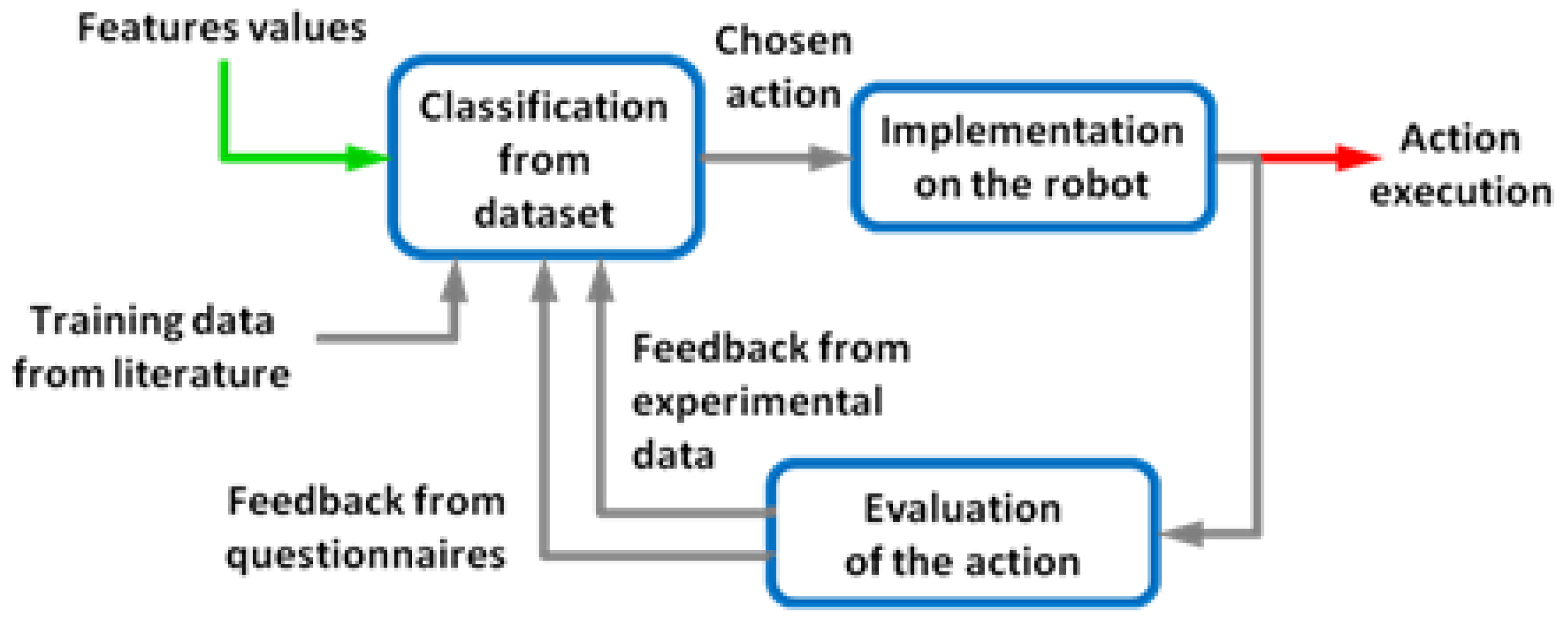
2.1. Generic Model

We want to implement a system that enables effective online learning for a robot by using data extracted from literature of human sciences as well as experimental data. In Figure 1, the concept is described: a table is made out of training data; features’ values are given as input, and the classifier outputs a chosen class that corresponds to an action to be implemented in the robot. The action is performed and evaluated through either questionnaires or experimental measurements. The resultant feedback updates the dataset.

2.2. Classification of Training Data

2.2.1. Characteristics of Data

In human-robot interaction and in social robotics, it is common to work with quantitative as well as qualitative data extracted from literature of studies of human sciences such as sociology, anatomy, anthropology, and so on. From these data we can extract features and classes; however, there are usually some properties that limit the possible choice of classifying methods:

• Heterogeneous data types: some features (such as gender) are binary values; some other (such as age) are continuous but can be discretized; some others (such as nationality) are categorical and not ordinal. Classes also can be represented in percentages or as absolute values, and features may be associated with more than one class to different degrees. Baynesian networks have been used to synthesize the findings from these separate studies of sociology, biology and economics [20], and can be used for representing and predicting social behaviors [21]. However, they assume parent/child relations between variables, while in our problem we are assuming independence between class-condition feature probabilities.
• Incompleteness: studies are usually focused on a single or a couple of specific variables, whereas our model involves more variables. For example, a study with gender as a variable, may fix some variables (e.g., nationality of participants) while not specifying others (e.g., education level) which might be of interest. Missing data can make it difficult to use techniques for classification such as neural networks or to even just represent it in a space with principal component analysis. See [22] for a review of the problem from a statistical perspective.
• Set size: Small datasets limit the choice of training methods. Data from different sources can be integrated in order to expand the training dataset, but this will also cause the incompleteness problem stated above. In particular, when integrating human studies data with experimental data, we receive the data incrementally (rather than in batch). Online learning methods fit this kind of problem. Small experimental datasets have been used in modelling of complex processes successfully in [23], but the composition of the training datasets becomes critical, with designed sets performing better than random ones. Other learning models were compared for problems with small datasets in [24], where mixed results were found dependent on feature selection, and naive Bayes and its multinomial variation [25] were reported to outperform the others, including support vector machines, in many conditions.

Given these properties, we believe that the naive Bayes classifier is a good choice for dealing with this kind of data. Naive Bayes can easily handle weighted data, incomplete data, small datasets, and categorical variables.

2.2.2. Naive Bayes

First, let us define the sets of features of our problem f = {f ₁, ..., f _I} and the sets of classes C = {C ₁, ..., C _J}, given I number of features and J number of classes. The dataset is composed of K elements < f ^(k), C^(k)>, resulting in {<f ⁽¹⁾, C⁽¹⁾>; ...; <f ^(K), C^(K)>}.

Equation (1) represents the generic formula of posterior probability for the class C_j and the feature f_i.

$$P\left(C_j|f\right)\propto P\left(C_j\right){\displaystyle \prod _{i}P\left(f_i|C_j\right)}$$

(1)

Naive Bayes is a simple generative probabilistic classification model which assumes independence between features of the objects to be classified [26]. Therefore, the naive Bayes classifier applies Bayes’s theorem with the assumption that the presence or absence of each feature is unrelated to other features. Its effectiveness in classification has been proven despite its independence assumption [27]. Moreover, naive Bayes only requires a small amount of training data to estimate the parameters necessary for classification. These characteristics make it appropriate for the features of many problems in social robotics.

Under naive Bayes we label object C* according to Equation (2):

$$C*=\arg {\displaystyle \underset{C_j}{\max }}P\left(C_j\right){\displaystyle \prod _i}P\left(f_i|C_j\right)$$

(2)

where P(C_j) is the prior probability of class C_j and P(f_i | C_j) is the likelihood of class C_j with respect to feature f_i. In general, these probabilities are estimated from the feature-class co-occurrence count table, e.g., using the maximum likelihood estimates as in Equation (3):

$$P\left(f_i|C_j\right)=\frac{count\left(f_i,C_j\right)}{count\left(C_j\right)}$$

(3)

The prior probabilities can be similarly derived from a count table. Thus these count tables form the sufficient statistics for the naive Bayes model. Count tables can be easily updated online, by simply incrementing class-feature counters, as each labelled example is processed, and the updated model can be immediately used for classifying new objects. In fact, the naive Bayes’s sufficient statistics form an additive monoid, and admit both efficient online training and efficient parallel learning [28].

2.3. Conversion of Heterogeneous Data into a Dataset

When handling real data from different sources, we should distinguish the types of studies we are using in order to clearly define a semantics of weights w_j that can be associated with classes C_j and build a count table which will serve as a batch for training. Data can appear in different types, such as:

(a)

A percentage in which all (and only) the classes of our problem are considered (ideal).

(b)

A percentage in which one or more classes of our problem are not considered.

(c)

A percentage in which one of the classes (defined as “other”) may include the classes of our problem which are not specifically mentioned.

(d)

Absolute values of measurement without a known scale (e.g., “15 times”).

(e)

Absolute values of measurement, between a priori maximum and minimum values (e.g., “24 out of 30”). Likert scales and differential semantic scales fall into this category.

Case (a) is the simplest, as percentages are directly turned into weights between 0 and 1. For example, in a study in which 55% of the population belongs to class C_A, its w_A will be 0.55.

For case (b), let us now consider the following simple sample data:

• Study 1: when feature 2 is 0, 55% of the population belongs to class C_A and the rest to class C_B, whereas when feature 2 is 1, the results change to 39% and 61%.
• Study 2: under different conditions (feature 1 = 1) and feature 3 fixed to 0, 50% of the population belongs to class C_B, and the rest to classes C_A and C_C.

In

Table 1. A portion of raw training data.

Feature 1	Feature 2	Feature 3	Class Label	Weight
0	0	unknown	CA	0.55
0	0	unknown	CB	0.45
0	1	unknown	CA	0.39
0	1	unknown	CB	0.61
1	unknown	0	CA	0.25
1	unknown	0	CB	0.5
1	unknown	0	CC	0.25

, we organized these data, marking the field as “unknown” where variables are not considered in the study. When some conditions significantly change between two studies, the index of the considered study itself should be considered a feature.

Normalization is then necessary, because data refer to different scales in which different classes were involved. In this case, class C_C is not present in the first study. Therefore, assuming a uniform prior estimation for the class C_C as 1/J, where J is the number of classes, the weights for C_A and C_B can be normalized to sum 1. In the above case where w_A = 0.39 and w_B = 0.61, they will be reduced to 2/3 (as 1/3 is a prior estimation of w_C), becoming w_A = 0.26 and w_B = 0.41.

The way of assuming a prior estimation for the missing class depends on the interpretation of the data, and cases (c), (d) and (e) differ from (b).

In Figure 2 we show an excerpt from three different empirical studies [29,30,31] (dating up to 1983) on asymmetry in facial expressions which provide different data, respectively focusing on (c) culture, emotion, and its background meaning; (d) asymmetry, gender and emotions; and (e) emotional valence, gender and asymmetry. Typically, a possible purpose of gathering these data could be making a robot capable of autonomously determining when an asymmetrical facial expression is appropriate.

In case (c) it may be desirable to split the remaining part to all the classes not specifically mentioned. For example, (as in Figure 2c, Happiness-Wisconsin) if the data reports 58.3% class C_A, 16.7% class C_B, 11.1% class C_C, and the remaining 13.9% other, supposing that our problem has five classes, the latter part can be approximated as the sum of the weights of classes C_D and C_E. Filling w_D = 0.0695 and w_E = 0.0695 and adding this data to the dataset will force these weights to be low, where a uniform estimation of 0.25 would be considered too high.

In case (d), in which, as in Figure 2, the number of subjects are counted, it is enough to apply the same method as (b), assuming a uniform prior estimation for the missing classes as 1/J.

Figure 2e shows an example of values measured in pixels, therefore having a maximum and minimum value: data vary within that scale. In this case it may be more reasonable to assign the average value of the scale to unknown classes. A further example with simpler data can clarify better the reason of this approach in case (e). In a problem with four classes with two of them unknown, a data vector could be <18/30, 24/30, ?, ?>, which equals <0.6, 0.8, ?, ?>. Fixing a uniform estimate of 0.25 (as in case (d)) for w_C and w_D, and then normalizing only w_A and w_B, the weights vector would result in <0.21, 0.29, 0.25, 0.25>: having w_C and w_D higher than w_A may not be reasonable. Instead, assuming data for C_C and C_D as 15/30 (the average value), adding the resulting w_C = 0.5 and w_D = 0.5, to the dataset and then normalizing it will force them to be higher: the weights vector would be <0.25, 0.33, 0.21, 0.21>. How the relative weight of w_A changes compared to unknown classes proves the importance of the semantics.

In all the above cases, after calculating the unknown weights, their addition to the dataset is not strictly necessary for the naive Bayes classifier to work, but it does become necessary depending on the policy described in Section 2.6.1.

2.4. Customisation of Naive Bayes Formulas

In our naive Bayes classifier, the selection of the class C* is done through a formula different from the standard one.

2.4.1. Conditional Probability

First, the standard formula of conditional probability is rewritten in Equation (4), taking into account the fact that class membership is based on weights w. The probability of f_i, the i-th feature of f, being equal to a value v, is found through the sum, for each k-th sample < f ^(k), C^(k)> in the dataset, of the weights that are defined when f_i = v through a multiplier δ ^(k)(v) (which can be 0 or 1). The formula of class priors P(C_j) is rewritten in the same way in Equation (5).

$$P\left(f_i=v|C_j\right)=\frac{{\displaystyle \sum _{k=1}^K\left({\delta }^{(k)}(v)\cdot w_j^{(k)}\right)}}{{\displaystyle \sum _{k=1}^K{w}_j^{(k)}}}$$

(4)

$$P\left(C_j\right)=\frac{{\displaystyle \sum _{k=1}^K{w}_j^{(k)}}}{K}$$

(5)

The best class C* is selected through Equation (6):

$$C*=\arg {\displaystyle \underset{C_j}{\max }}P\left(C_j\right){\displaystyle \prod _{i=1}^{I}P\left(f_i=v|C_j\right)}$$

(6)

In our customized formula (Equation (7)), we leave class priors P(C_j) out. This additional assumption is made because we do not want to give more weight to more common class a priori, so only independent probability distributions are considered.

$$C*=\arg {\displaystyle \underset{C_j}{\max }}{\displaystyle \prod _{i=1}^{I}P\left(f_i=v|C_j\right)}$$

(7)

Leaving out the class priors is equivalent to assuming a uniform probability distribution over the classes. Class distributions estimated from very small samples are inherently noisy, and we believe using a flat prior here is a legitimate choice. An example can clarify the need for this modification. The typical case is when having a very small dataset, like the one in

Table 2. A portion of training data, shown as sample.

Feature 1	Feature 2	Feature 3	Class Label	Weight
0	1	1	1	0.2501
0	1	1	2	0.2497
0	1	1	3	0.2502
0	1	1	4	0.2500
1	1	0	2	0.5000

, in which one class appeared more times than the others.

Using the classification formula of Equation (6), the mapping of the maximum likelihoods for each possible combination of features would result as in

Table 3. Examples of mapping depending on class priors.

on the left. The bias towards class 2 comes from the priors P(C_j), which would be <0.2501, 0.3749, 0.2502, 0.2500>. Without such bias, the mapping will appear as in Table 3 on the right. Extending the concept to a bigger mapping, it is easy to predict that priors can unbalance it and penalize less common classes, which may never be selected.

2.4.2. Smoothing Technique

Conditional probabilities P(f_i | C_j) are balanced out through an add-ε smoothing technique, namely the use of m-estimate [32], which avoids the inconveniences that may happen when the number of total occurrences of a feature under certain conditions equals 0. In generic terms, for estimating conditional probabilities in a table of data, instead of using the standard formula in Equation (8), the formula in Equation (9) is used. The probability of A given B does not depend only on the joint probability of A and B divided by the probability of B, but is balanced out by p and m. We need p as a non-zero prior estimate for P(A | B), which we suppose uniformly distributed, and a number m that says how confident we are of this prior estimate p.

The value m is defined as the equivalent sample size of m-estimate formula. It can be tuned on a development set; usually a small number is convenient for small sets of data, in order to balance out probability from training data compared to the weight of p. The value p is the uniform prior estimation of the probability. It is usually set as 1/J, where J is the number of classes.

$$P\left(A|B\right)=\frac{P\left(A\cap B\right)}{P\left(B\right)}$$

(8)

$$P\left(A|B\right)=\frac{P\left(A\cap B\right)+m\cdot p}{P\left(B\right)+m}$$

(9)

As a result, the generic formula of the classifier is shown in Equation (10):

$$P\left(f_i=v|C_j\right)=\frac{{\displaystyle \sum _{k=1}^K\left({\delta }^{(k)}(v)\cdot w_j^{(k)}\right)}+m\cdot p}{{\displaystyle \sum _{k=1}^K{w}_j^{(k)}}+m}$$

(10)

2.4.3. Incomplete Data

As we may have to deal incomplete data, the multiplier δ ^(k)(v), a function introduced for the calculation of the joint probability of a certain feature with a certain class, can be customized as well, as in Equation (11).

Depending on the quantity of incomplete training data, δ ^(k)(v) can be defined arbitrarily. It can be 0.5 or even less, in case incomplete data is considered not reliable.

$${\delta }^{(k)}(v)=\{\begin{array}{cc}1& f_i^{(k)}=v\\ 0.5& f_i^{(k)}=\text{undefined}\\ 0& \text{otherwise}\end{array}$$

(11)

2.5. Adaptation through Rewards

In our model, the representation of knowledge has to be adaptive to feedback collected from experimental data. Therefore, the model includes rewards or penalties depending on the feedback.

Ideally, the algorithm has to adapt quickly. As in human-robot interaction where we are dealing with real world problems rather than abstract ones, the desired amount of iterations necessary for a complete adaptation from the initial mapping to another one should be comparable to the number of interactions humans need to understand behavior rules. The process should not require hundreds or thousands of steps.

Each time a class is selected and an action is executed by the robot, probabilities of the current data sample <f *, C*> at step T are considered weights and updated to the new weights at step T + 1 through the formula in Equation (12).

$$w(T+1)=w(T)+l\cdot r\cdot d$$

(12)

The learning rate l, the reward factor r and the value d depend on the specific implementation.

For instance, if the feedback data is obtained from 5-point Likert scales, r could be a value among {−1, −0.5, 0, 0.5, 1} depending on the questionnaire results, whereas d could be 1−w(T) or w(T) depending on the questionnaire feedback being >3 (positive reward) or <3 (negative reward). Otherwise, if feedback is obtained from experimental data such as measurement of participant’s response of some kind, the formula for r could be tailored to be proportional to performance such as the success of an action, the number of hits, or inversely proportional to negative performance such as delay of response. Through the combination of these factors, a cost/reward function can be tailored for the experiment.

The learning rate l can be kept at 1 for assigning equal importance to each step. The adapting process can be forcefully led to convergence if l is a decreasing function instead (for example, following the e^−x curve), when real world scenario constraints make it necessary.

Rewards are commonly used in reinforcement learning too, where transitions from states to other states happen through a range of actions: rewards affect good states or actions when the goal is reached. In our case, rewards modify the weight actions associated to states, but there is no transition between one state and another: one whole iteration consists in just one state, defined by current feature values.

2.6. Other Policies

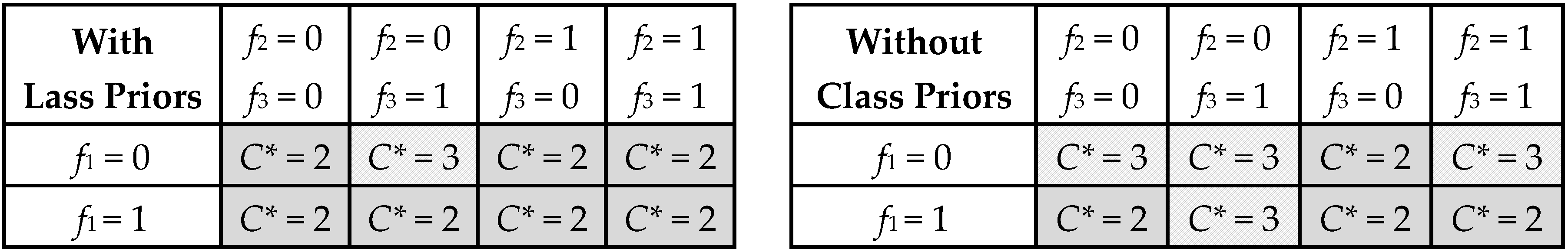
2.6.1. Class Selection

Whenever a new vector of input features f* has to be classified, the following cases may happen:

• The set of features f* is not present in the dataset. In this case, naive Bayes is calculated.
• The set of features f* is already present in the dataset and the vector is associated with some weights. In this case, classification can be done either by:

  o

  using the current weights: generically speaking, in order for this option to be possible, data has to be consistent within all classes for f*, with missing data previously filled as explained in Section 2.3.

  o

  ignoring the current weights, and recalculating the probabilities through naive Bayes (leave-one-out cross-validation [33]).

Regardless of the vector of the current input features f* corresponding to a vector of new probabilities or to a vector of previous weights, in either case there are several possible policies for the selection of the output class C*:

• The simplest solution is to get the maximum value, as in the standard Equation (6) and Equation (7).
• Another possibility, which gives more emphasis to exploration, is to use a ε-greedy policy: with 0 < ε < 1, C* is the argmax with ε probability, and will be a random selection with 1 − ε probability.
• C* can be assigned any of the possible classes, with probability proportional to the list of weights. For example, in a weight vector <0.4, 0.2, 0.1, 0.3>, the first class would be selected with 0.4 probability.

2.6.2. Stopping Conditions

The adaptation process can potentially be continuous, or can be stopped depending on criteria that are up to the experimenter. When stopping conditions are satisfied, rewards will no longer apply, and the system will be considered fully trained.

One possible method is to verify the maximum likelihoods for each possible combination of features. Making a mapping of such values, like in Table 3, we form a table in which each cell represents a “state” and is associated with an “action” represented by the class with maximum likelihood C*. Then, stopping conditions can be triggered when changes of C* are stabilized. This condition is verified when the following two conditions (Equations (13) and (14)) are true at the same time. One condition ensures that all states have been explored once (there is at least one entry k of the dataset, defined as <f ^(k), C^(k)>, in which f ^(k) corresponds to that features vector). The other condition checks whether the moving average of C* changes during the latest W (window length) iterations to decrease below a threshold.

$$\forall f,\exists k:f^{(k)}=f$$

(13)

$$\frac{{\displaystyle \sum _{t=T-W+1}^T\frac{{\sigma }_C}{{\sigma }_{TOT}}}}{W}\le \theta$$

(14)

In Equation (14), σ_C is the number of states in which C* changed; σ_TOT is the total number of states. The threshold θ can be set as $\raisebox{1ex}{$q$}\!\left/ \!\raisebox{-1ex}{${\sigma }_{TOT}$}\right.$ (tolerance of average q changes, with q to be determined according to the desired convergence).

3. Results and Discussion

In this section we will describe two applications of the algorithm. We will not enter into detail of the research behind those experiments, but rather show the effectiveness of our method. In both applications, some details of the algorithm have been customized. Discussion follows in the last part.

3.1. Application 1: Greeting Interaction

3.1.1. Purpose of the Study

As humans, we greet each other following sometimes complex or unclear rules which vary by country or even by region. Nevertheless, when exposed to a new culture, we are able to adapt to a new set of rules after only a few interactions. The purpose of this study was to make a humanoid robot adapt to the German way of greeting, while being initially trained with Japanese social data about greeting rules. Culture differences are indeed important for ensuring technology acceptance [34], including more complex machines such as robots. In a recent work, Heenan et al. made a state machine model for greetings comprehensive of the approach phase [35]; however, it does not take cultural factors into consideration, which is the focus of this experiment. ARMAR-III [36], a humanoid robot designed for close cooperation with humans, was used in this experiment, which took place in the room shown in Figure 3.

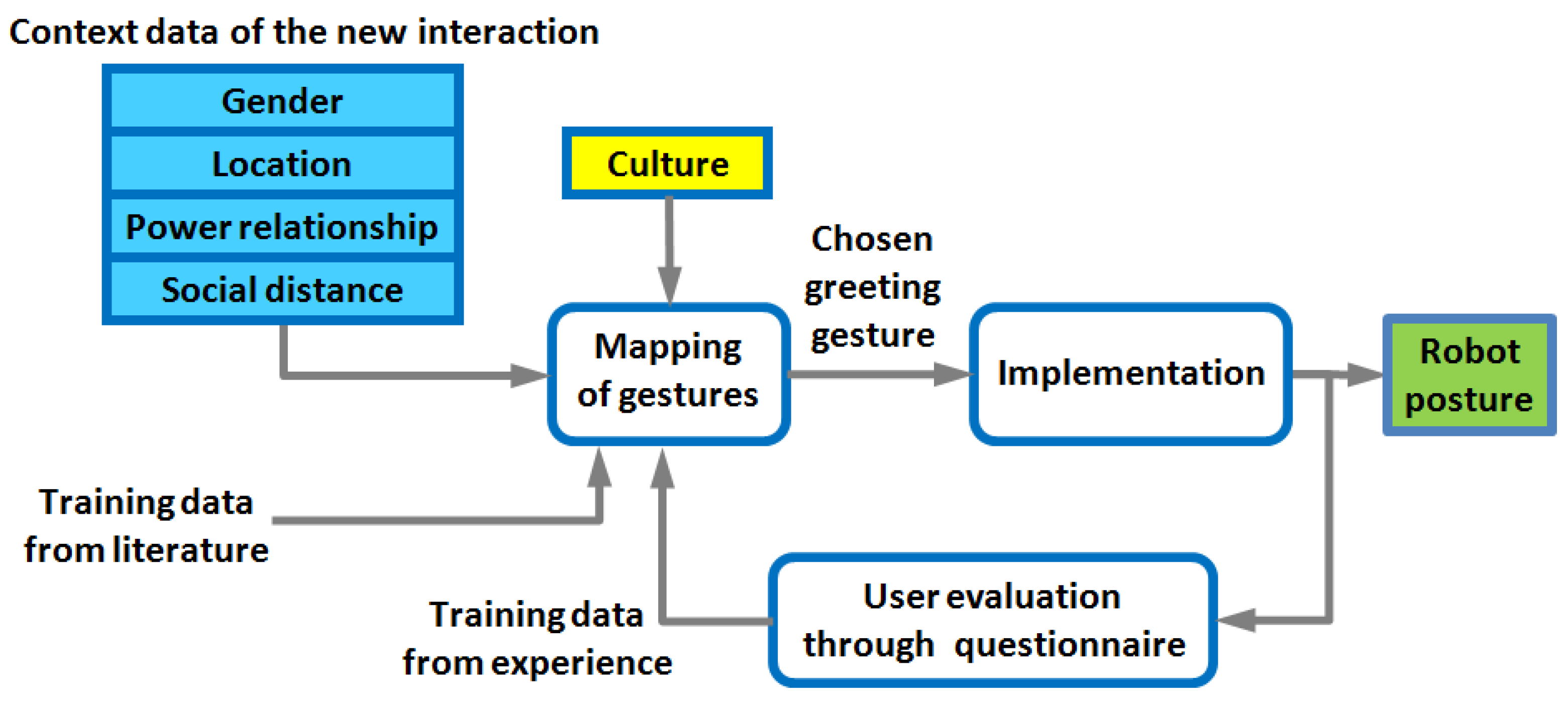
3.1.2. Greeting Selection System

The implementation of the greeting selection system is composed of two parts regarding gesture and speech; in Figure 4 and in the next paragraph we describe only the part related to gestures.

The system takes context data (in blue) as input features and produces the appropriate robot posture for that input. Robot posture configuration is implemented through a process described in [18].

The values of features and classes regarding greeting gestures is summarized in

Table 4. Feature values and classes of the greeting gestures model.

Context (Features)	Feature Values	Greeting Types (Classes)
Gender of the human partner	0. Male 1. Female	1. Bow
Location	0. Private 1. Public 2. Workspace	2. Nod
Power relationship	0. Inferior 1. Equal 2. Superior	3. Raise hand
Social distance	0. Close 1. Acquaintance 2. Unknown	4. Handshake
Discriminant	Values	5. Hug
Culture	0. Japanese 1. German

. As the experiment consists of adapting from knowledge extracted from one culture (Japanese) to another (German), culture acts as a discriminant rather than being an input feature. In this way, for different cultures, there will be different mappings.

Mappings are updated using experimental data in the form of questionnaires filled by experiment participants. In order to be initialized, the only needed training set is the Japanese one: before beginning the experiment, a table made from Japanese sociology data and a mapping called M0J was built. After interacting with German people, the resulting adapted mapping M1 is expected to represent German rules of greeting interaction. A mapping M0G made from a table of German sociology data of gestures was built, too, and only used for validation. Our hypothesis is that M1 will be closer to M0G than to M0J.

3.1.3. Rewards Calculation

Following Figure 5, let us summarize the concept of the algorithm and the way rewards are calculated:

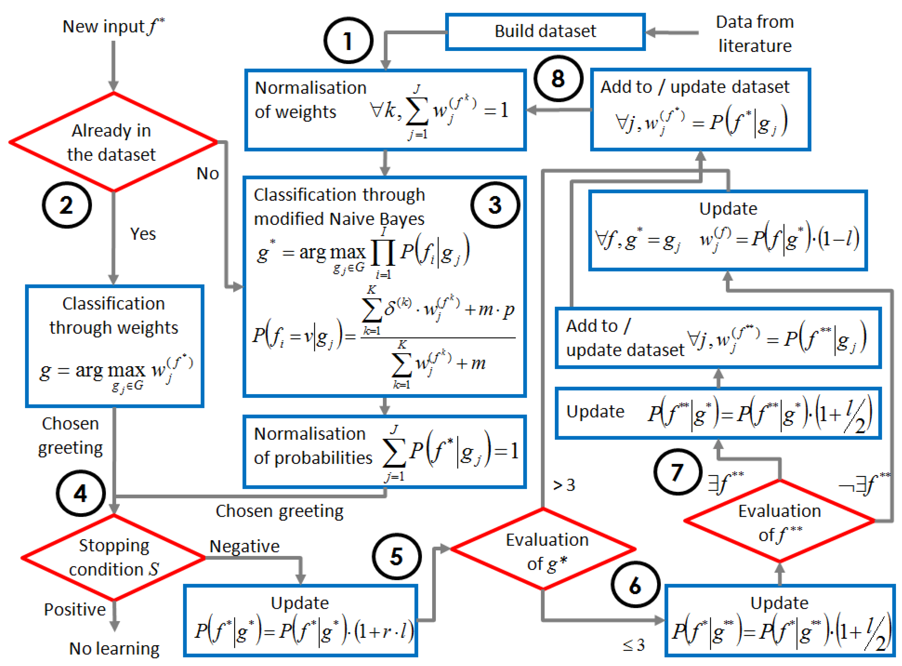
• The dataset is built from training data: weights w_j^(f) corresponds to each vector added.
• Whenever a new feature vector f* is given as input, it is checked whether it is already contained in the dataset or not. In the former case, the weights are directly read from the dataset and the greeting corresponding to the highest weight is selected; in the latter case, classification is calculated through naive Bayes.
• In the naive Bayes classifier, the best greeting g* chooses the greeting g_j that has the highest probability, calculated from its weights w_i, using the add-ε smoothing technique and a multiplier δ, as in Equation (10).
• Once the greeting is chosen, the resulting probabilities are normalized. The stopping condition is then calculated as in Equations (13) and (14). If all conditions are satisfied, no updating will be performed, as the mapping has already been stabilized.
• Otherwise, the next step consists of getting the evaluation from the participant for the current selected greeting g*, whether appropriate or not according to the participant’s culture, to the current context f*. On a scale from 1 to 5, if it is greater than 3, the weight of that greeting for the present context is multiplied by a positive reward. If less than 3, is it multiplied by a negative reward; if it is exactly 3, nothing is done. All vectors f start with a counter s set to 0, and every time one vector is processed, its counter increases and makes the learning factor decrease, dampening the magnitude of the rewards.
• If the evaluation is less than or equal to 3, the participant is also asked to indicate which greeting type instead would have been appropriate in this context f*. The weight of that greeting g** is boosted.
• The participant is finally asked to indicate, for the chosen greeting type g*, which context f** would have sounded appropriate. If there is any, the weights corresponding to f** are updated with a boost for the current greeting; otherwise, if g* is judged inappropriate in any case, all the weights receive a negative reward. The vector f** is added to the dataset if new, or updated if already existing.
• All the new weights in the dataset are normalized (the sum of all probabilities of greeting types for a single context combination has to be 1). At this point, the algorithm is ready for a new input, and goes back to step 1. The next time that the input feature vector is the same as the one just added, the weights will be directly used (step 2 instead of 3).

As explained in steps 4, 5 and 6, the questionnaire is made up of three questions; this means that at the same time the rewards may affect directly three weights in two cells of the mapping (and indirectly all the others), making the learning process much faster.

K	Number of samples in the dataset	i = 1 … I	Index of features
k = 1 … K	k-th sample <f, gj> in the dataset	f	Feature input vector
G	Set of greetings (classes)	fi	i-th feature of f
J = 5	Number of possible greeting choices	f (k)	k-th feature vector in the dataset
j = 1 … J	Index of greetings	f *	Feature vector selected by the classifier
gj	j-th greeting in G	f **	Feature vector suggested by the participant to match g*
g(k)	Greeting at the k-th element in the dataset	v	Value that can be taken by a feature fi
g*	Greeting chosen by the classifier	wj (f)	Weight of the gesture j for the feature vector f
g**	Greeting chosen by the participant in case g* receives a low score	m = 2	Equivalent sample size of m-estimate formula
I = 4	Number of input features	p = 1/J	Uniform prior estimation of the probability
s	Counter of visits of the current f*	r ={1, 0.5, 0, −0.5, −1}	Reward factor, depending on the evaluation of the user
l =exp(–s/4)	Learning factor. High (around 0.8) at the beginning and decreases following the e-x curve	S	Stopping conditions as in Equations (13) and (14), with W = 10 and q = 2/σTOT
δ(k) = {1, 0.2, 0}	Multiplier for incomplete data, as in Equation (11). Set empiricallylow in case of undefined fi, due to the high quantity of incomplete training data

3.1.4. Experiment Results and Validation

In this experiment, 18 German people of different ages, gender, workplace, and knowledge of the robot were invited to participate. Some of them participated in a second interaction. At the end, all the feature values had the chance to be classified at least once except for “Location = Private.”

The number of interactions, including repetitions, was 30: it was determined by the stopping condition of the algorithm. Each time a state, determined by a combination of feature values, had its weights modified during the feedback after each interaction, it is counted as “visited.” The count of how many times states have been visited is shown in

Table 5. Count of visited states at T = 30.

		Close	Close	Close	Acquain.	Acquain.	Acquain.	Unknown	Unknown	Unknown
		Inferior	Equal	Superior	Inferior	Equal	Superior	Inferior	Equal	Superior
Public	Male	1	1	1	4	7	2	6	7	4
Public	Female	0	3	0	2	2	2	4	4	4
Workplace	Male	1	1	5	3	4	3	3	3	4
Workplace	Female	0	0	3	3	9	3	4	6	5

.

The new mapping of gestures was verified through an objective function V described in the generic Equation (15), which measures the difference between two different mappings, M1 and M2.

$$V={\displaystyle \sum _f{\displaystyle \sum _j{\left(w_j^{(M{1}_f)}-w_j^{(M{2}_f)}\right)}^2}}$$

(15)

The function calculates the sum of the variance between the weights w in the same features vector f in two different mappings, M1 and M2. Each variance in the weights is calculated not only by comparing the greeting with maximum likelihood, but also considering the sum of the variances for each greeting j.

The function applied to M0J (Japanese initial mapping) and M1 (final mapping) gives 0.636 as the result. Conversely, comparing M1 with M0G (German initial mapping), 0.324 is obtained. The t-test of the variances for each f proves the difference to be significant (p = 0.02), validating the hypothesis that M1 would become closer to M0G than to M0J. This result supports the evolution of mapping M1 from M0J towards M0G, assuming that M0G represents German rules correctly: the robot learned a gesture for each social context that is close to the German and more appropriate than the Japanese one. How weights evolve is shown in Table 6 and Table 7, where on the left the tables are at the starting condition (Japanese): on the right, variances decrease in Table 6 and increase in Table 7.

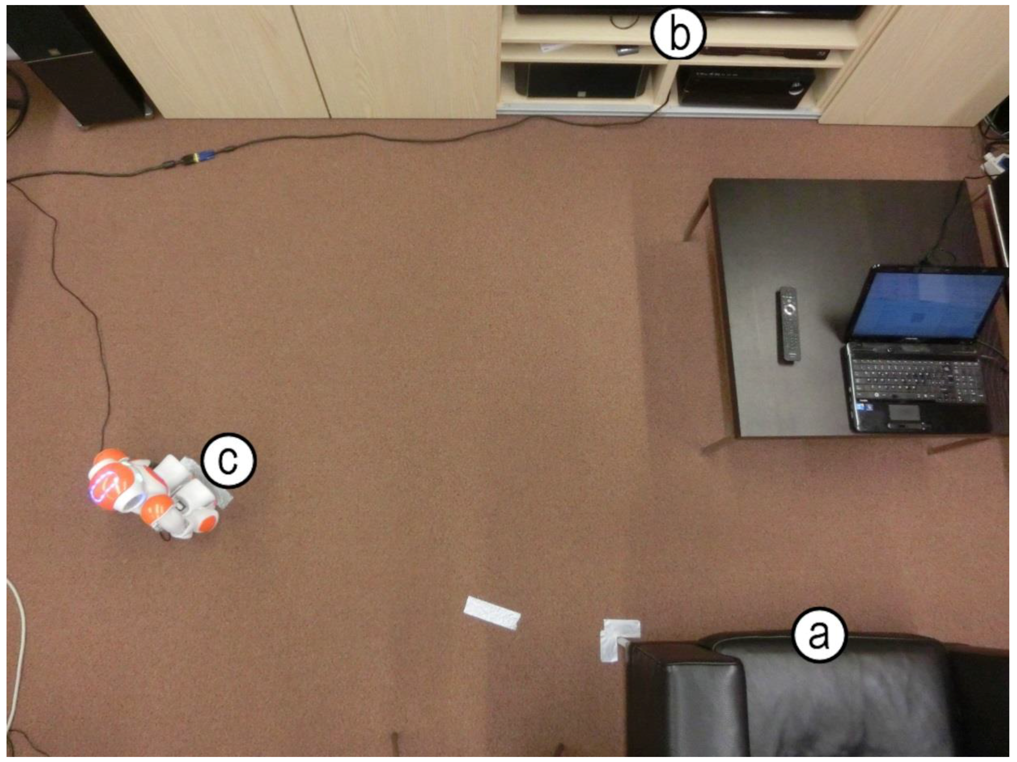
3.2. Application 2: Attracting Attention

3.2.1. Purpose of the Study

Socially assistive robots [37] are a category of robots that can actively assist humans (especially elderly people) thanks to their ability of navigation and their multimodal communication capabilities. However, in order to communicate with a human partner, the robot needs to attract human’s attention. Different modalities of communication have been evaluated [38] and compared with multimodal communication cues [39]. The purpose of the present experiment is to explore strategies for successfully initiating communication with humans in a changing environment, making a robot learn which communication channel is more effective for each condition of the room where the interaction occurs. The social robot Nao [40] was used for this application, which was divided in three separate experiments (one of them published in [19]), with different conditions among them. We will examine in detail only the first one.

3.2.2. Experiment Design

The robot Nao is placed in a room (Figure 6), which is adjusted to the actual manipulated conditions which are the features in

Table 8. Feature values and classes of the attracting attention problem.

Room Conditions (Features)	Feature Values	Behaviors (Classes)
Loudness	0. Quiet 1. Loud	1. Blinking 2. Waving 3. Beeping 4. Walking 5. Pausing TV
Ambient luminance	0. Light 1. Dark
Distance	0. Far 1. Close
Number of individuals	0. Robot + participant 1. One additional person

(dark/light, loud/quiet and so on). While the participant is concentrated watching TV, at random intervals one of the behaviors listed in Table 6 will be triggered and Nao will try to attract the person’s attention until he/she pauses the TV.

The three experiments mainly differ in:

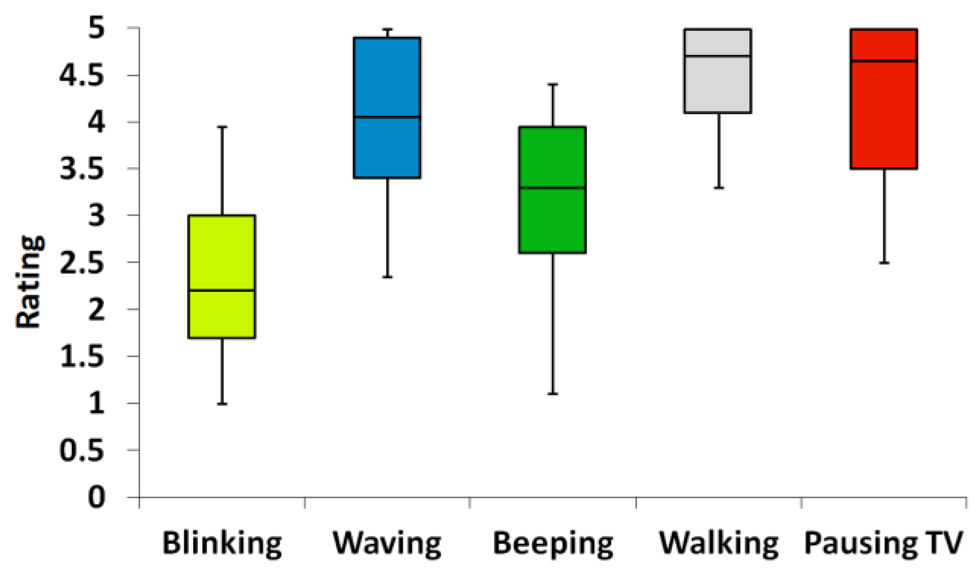
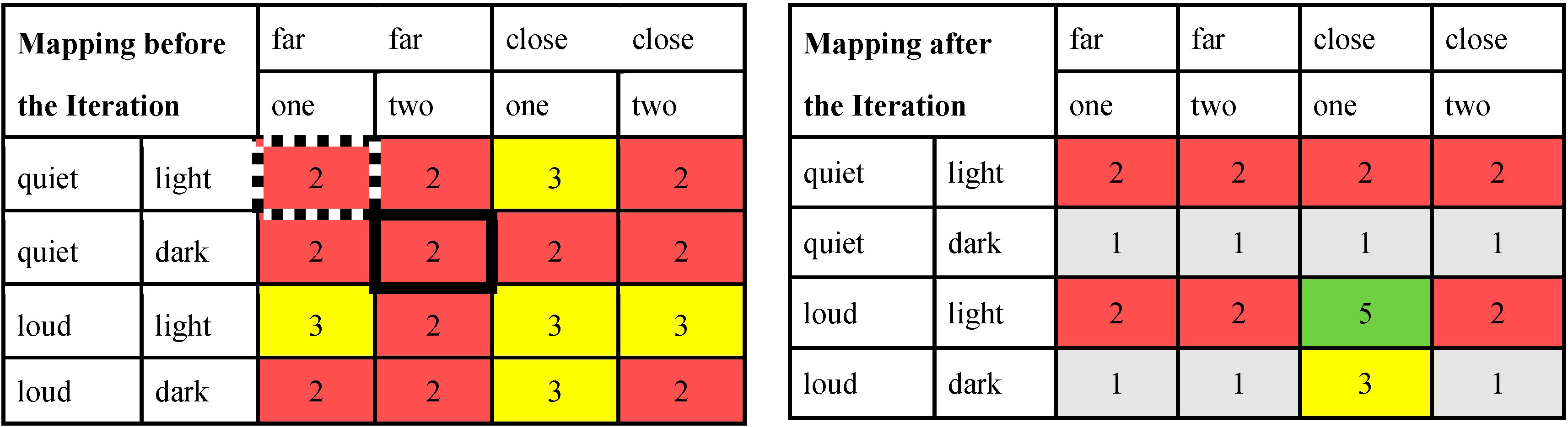
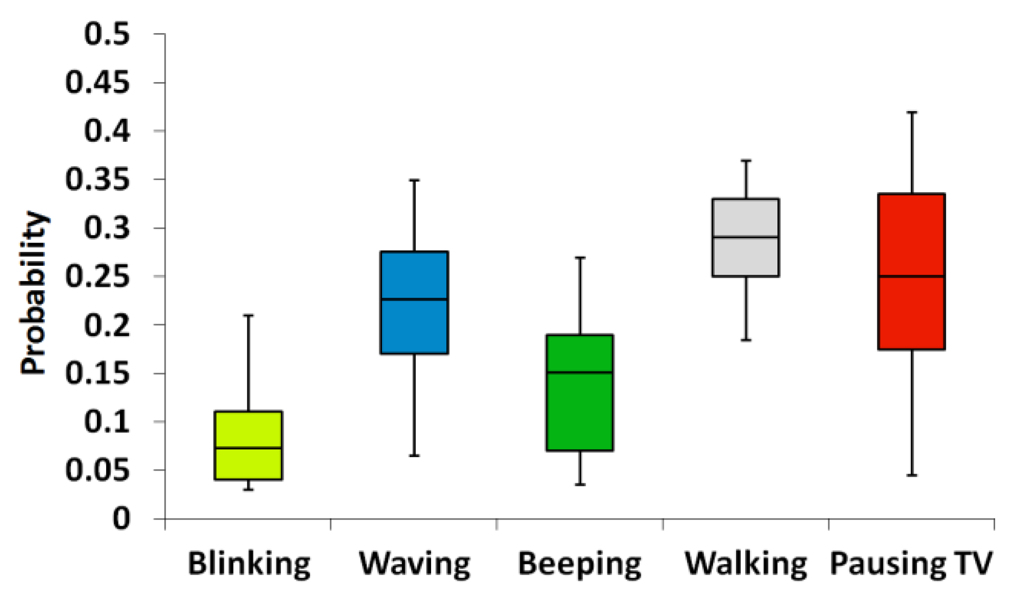
• Features and classes: the room conditions and possible behaviors listed in Table 8 refer to the first session. As all the features are binary, the mapping is composed of 16 possible combinations. The third experiment had a smaller number of features (three for a total of 12 combinations) and four behaviors.
• Measurement: in the first two experiments, feedback is provided by a questionnaire that is filled out every time the TV is paused. It is based on 5-point semantic differential scales, similar to the experiment in Section 3.1. In the third experiment, feedback comes from a cost/reward function calculated from other measurements such as reaction times, head direction, delay and a fixed cost of each of the robot’s behaviors. These factors are grouped as reward for action r_A, which is positive or null; cost for the robot c_R (depending on how expensive an action is); and cost for the human c_H (measuring how much the human lost concentration).
• Class selection policy: in the third experiment we used leave-one-out cross-validation introduced in Section 2.6.1: classification is never taken directly from the current weights, but naive Bayes probabilities are recalculated every time, leaving the current features’ input out of the calculation.

3.2.3. Settings of the Algorithm

The architecture of the algorithm is similar to the one in Section 3.1.3. It can be summarized as follows:

• The dataset of experience is initially empty. Whenever a new feature vector is given as input, it is checked whether it is already contained in the dataset or not. In the former case, the classification happens reading the weights directly from the dataset; in the latter case, they get assigned the values of probabilities calculated through our customized naive Bayes of Equation (10).
• Once the behavior b* is chosen and executed, we get the evaluation, on 5-point semantic differential scales, from the participant:

  • whether b* was effective or not;
  • if the evaluation was lesser or equal than 3 at point a, which behavior type b** instead would have been appropriate in this context f*;
  • if the evaluation was lesser or equal than 3 at point a, in which context f** the behavior b* would have been effective.
• Weights are updated through the formula of Equation (12) w(T + 1) = w(T) + l · r · d where T is the current time step, l = exp(–s/4) is the learning factor (proportional to s, the counter of visit of each state), r is the reward factor {−1, −0.5, 0, 0.5, 1} depending on the rating, and d is 1−w(T) or w(T) depending on the rating being greater/lesser/equal to 3.
• New data obtained from these evaluations are then added to the dataset and normalized.

As in the previous experiment, this way of managing the questionnaire allows data from experience to affect the mapping in up to two different cells at the same time. Next, we report the main differences:

• Unlike in Section 3.1, in which the adaptation process was incremental for all participants, here we ran a separate whole set of interactions for each participant. This makes it possible to distinguish actual learning regardless of personal differences among participants. As for each one we fixed 12 iterations, there were no stopping conditions.
• There is no batch data for training. The mapping starts untrained, and this brings some complications. Initializing the first input vector with random values makes learning biased towards the classes that are (even slightly) more likely at the very beginning. Subsequent positive reward may cause a lack of exploration. This problem can be solved using a different policy of class selection, as explained in Section 2.6.1, such as ε-greedy, and/or removing the bias of the class priors, as introduced in Section 2.4.1. A stronger effect can even be obtained if the priors are replaced by another function that actuates a counter-bias.

3.2.4. Results

Each of the 23 participants performed 12 repetitions of the interaction. We expected the algorithm to update the mapping and effectively represent participants’ preferences. Another 25 participants were used as the control group, receiving six randomly chosen actions instead of those generated from the algorithm.

First, we show in

Table 9. Evolution of maximum likelihoods for one iteration.

an example of how mapping can evolve in one iteration. In the situation of the mapping on the left, values have been assigned based on one random input vector (its weights are around 0.2 + ε). The state (quiet; dark; far; two) gets evaluated: the subject assigns a low score (<3) for the behavior 2 (waving), suggesting 1 (blinking) with maximum score (5) and suggests the state (quiet; light; far; one) as appropriate for waving. The resulting mapping on the right shows how: other states were affected by the high rating of behavior 1 and 2 for respectively the second and fourth, and for the first and third row; how due to customization of priors in the equation, less likely behaviors (such as 5) may appear again.

In order to assess the effectiveness of learning, the final probability matrix distribution and the average rating distribution of every behavior in the questionnaires were compared. A correlation test was conducted and we found a positive correlation (Pearson correlation of 0.716), proving that the preferences of the participants were learned. Figure 7 and Figure 8 show the variation of average ratings and respective probability distributions for every action. This essentially means that the robot has learned to adapt its attention-attracting behavior selection to the evolving context.

3.3. Discussion

3.3.1. About this Approach

The term “machine learning” was not used in this paper to refer to our solution, which is more appropriately referred to as “statistical learning.”

We believe the advantages of our approach are its feasibleness and its potential to be used by other researchers, tuning it according to their needs, especially if the datasets are made of heterogeneous or incomplete knowledge, and if the goal is to adapt through experimental data. Other more refined machine learning solutions are more appropriate for other kinds of studies, in which the focus is not on interaction and the learning problem is more complex.

This solution has also the advantage of being independent from the implementation and of not being robot-specific. Its limitation is the consequence of such an advantage: if the algorithm is implemented separately, its integration with the robot’s environment is also necessary every time.

3.3.2. Customization

The method we proposed can be customized and extended. In the applications described, the following variations were attempted:

• One feature turned into a discriminant in order to have two separate mappings
• Adaptation of one mapping made from literature to a new one VS adaptation without training dataset
• Rewards affecting more than one cell of the mapping through questionnaires
• Training data: from literature of human studies VS from corpora VS from experimental data
• Reward: from questionnaires VS from cost function
• Learning: incremental for all participants VS separate for each participant
• Class selection: using directly the weights VS leave-one-out cross-validation
• Class priors left out of the probability formula: alternative solutions are possible, such as a function that biases towards low probability classes using the inverse of the priors, or towards the classes that have been selected fewer times.

4. Conclusions

An adequate level of cognition is necessary to employ a robot in a human environment. There is a need of representing knowledge, which can be incomplete and heterogeneous, in an effective and efficient way. Adaptation to changing environments can be carried out through different learning techniques, which can be more or less effective depending on the specific problem. This work introduces a quick and effective way of handling this kind of problem adaptation based on statistical learning, specifically on naive Bayes. The method we proposed was applied to two different experiments of human-robot interaction. In the first, the humanoid robot ARMAR-IIIb adapted its greeting behavior from the Japanese to German style, using Japanese sociology data as training. In the second, the robot Nao learned different ways of attracting human users’ attention depending on different contexts. In both cases, the adaptation process was successful. The proposed method can be customized and readapted to be used on other robots. Future works include comparison with other machine learning techniques.

References and Notes

- Wolpert, D.H. The Lack of a Priori Distinctions between Learning Algorithms. Neural Comput. 1996, 8, 1341–1390. [Google Scholar] [CrossRef]
- Nguyen-Tuong, D.; Peters, J. Model learning for robot control: A survey. Cogn. Process. 2011, 12, 319–340. [Google Scholar] [CrossRef] [PubMed]
- Rosenblatt, F. The perceptron: A probabilistic model for information storage and organization in the brain. Psychol. Rev. 1958, 65, 386–408. [Google Scholar] [CrossRef] [PubMed]
- Bottou, L. Large-Scale Machine Learning with Stochastic Gradient Descent. In Proceedings of COMPSTAT’2010, Paris, France, 22–27 August 2010; Lechevallier, Y., Saporta, G., Eds.; Physica-Verlag HD: Paris, France; pp. 177–186.
- Yu, H.-F.; Hsieh, C.-J.; Chang, K.-W.; Lin, C.-J. Large Linear Classification When Data Cannot Fit in Memory. ACM Trans. Knowl. Discov. Data (TKDD) 2012, 5, 23:1–23:23. [Google Scholar] [CrossRef]
- Kober, J.; Bagnell, J.A.; Peters, J. Reinforcement learning in robotics: A survey. Int. J. Robot. Res. 2013, 32, 1238–1274. [Google Scholar] [CrossRef]
- Floreano, D.; Husbands, P.; Nolfi, S. Evolutionary Robotics. In Springer Handbook of Robotics; Springer: Berlin/Heidelberg, Germany, 2008; pp. 1423–1451. [Google Scholar]
- Mnih, V.; Kavukcuoglu, K.; Silver, D.; Rusu, A.A.; Veness, J.; Bellemare, M.G.; Graves, A.; Riedmiller, M.; Fidjeland, A.K.; Ostrovski, G.; et al. Human-level control through deep reinforcement learning. Nature 2015, 518, 529–533. [Google Scholar] [CrossRef] [PubMed]
- Goodrich, M.A.; Schultz, A.C. Human-Robot Interaction: A Survey. Found. Trends Hum.-Comput. Interact. 2007, 1, 203–275. [Google Scholar] [CrossRef]
- Franklin, D.W.; Milner, T.E.; Kawato, M. Single trial learning of external dynamics: What can the brain teach us about learning mechanisms? Int. Congress Series 2007, 1301, 67–70. [Google Scholar] [CrossRef]
- Spronck, P. Adaptive Game AI. Ph.D. Thesis, Maastricht University, Maastricht, The Netherlands, 2005. [Google Scholar]
- Klingspor, V.; Demiris, J.; Kaiser, M. Human-robot communication and machine learning. Appl. Artif. Intell. 1997, 11, 719–746. [Google Scholar]
- Fong, T.; Nourbakhsh, I.; Dautenhahn, K. A survey of socially interactive robots. Robot. Auton. Syst. 2003, 42, 143–166. [Google Scholar] [CrossRef]
- Dautenhahn, K. Socially intelligent robots: Dimensions of human–robot interaction. Philos. Trans. R Soc. Lond. B Biol. Sci. 2007, 362, 679–704. [Google Scholar] [CrossRef] [PubMed]
- Myagmarjav, B.; Sridharan, M. Knowledge Acquisition with Selective Active Learning for Human-Robot Interaction. In Proceedings of the Tenth Annual ACM/IEEE International Conference on Human-Robot Interaction Extended Abstracts; HRI’15 Extended Abstracts. ACM: New York, NY, USA, 2015; pp. 147–148. [Google Scholar]
- Lepora, N.F.; Evans, M.; Fox, C.W.; Diamond, M.E.; Gurney, K.; Prescott, T.J. Naive Bayes texture classification applied to whisker data from a moving robot. In Proceedings of the 2010 International Joint Conference on Neural Networks (IJCNN), Barcelona, Spain, 18–23 July 2010; pp. 1–8.
- Lepora, N.F.; Pearson, M.J.; Mitchinson, B.; Evans, M.; Fox, C.; Pipe, A.; Gurney, K.; Prescott, T.J. Naive Bayes novelty detection for a moving robot with whiskers. In Proceedings of the 2010 IEEE International Conference on Robotics and Biomimetics (ROBIO), Tianjin, China, 14–18 December 2010; pp. 131–136.
- Trovato, G.; Do, M.; Kuramochi, M.; Zecca, M.; Terlemez, Ö.; Asfour, T.; Takanishi, A. A Novel Culture-Dependent Gesture Selection System for a Humanoid Robot Performing Greeting Interaction. In Social Robotics; Beetz, M., Johnston, B., Williams, M.-A., Eds.; Springer International Publishing: Sydney, Australia, 2014; pp. 340–349. [Google Scholar]
- Trovato, G.; Galeazzi, J.; Torta, E.; Ham, J.R.C.; Cuijpers, R.H. Study on Adaptation of Robot Communication Strategies in Changing Situations. In Social Robotics; Tapus, A., André, E., Martin, J.-C., Ferland, F., Ammi, M., Eds.; Springer International Publishing: Berlin/Heidelberg, Germany, 2015; pp. 654–663. [Google Scholar]
- Levontin, P.; Kulmala, S.; Haapasaari, P.; Kuikka, S. Integration of biological, economic, and sociological knowledge by Bayesian belief networks: The interdisciplinary evaluation of potential management plans for Baltic salmon. ICES J. Mar. Sci. 2011, 68, 632–638. [Google Scholar] [CrossRef]
- Whitney, P.; White, A.; Walsh, S.; Dalton, A.; Brothers, A. Bayesian Networks for Social Modeling. In Social Computing, Behavioral-Cultural Modeling and Prediction; Salerno, J., Yang, S.J., Nau, D., Chai, S.-K., Eds.; Springer: Berlin/Heidelberg, Germany, 2011; pp. 227–235. [Google Scholar]
- Ghahramani, Z.; Jordan, M.I. Learning from Incomplete Data. 1995. Available online: http://dspace.mit.edu/handle/1721.1/7202 (accessed on 20 January 2016).
- Lanouette, R.; Thibault, J.; Valade, J.L. Process modeling with neural networks using small experimental datasets. Comput. Chem. Eng. 1999, 23, 1167–1176. [Google Scholar] [CrossRef]
- Forman, G.; Cohen, I. Learning from Little: Comparison of Classifiers Given Little Training. In Knowledge Discovery in Databases: PKDD 2004; Boulicaut, J.-F., Esposito, F., Giannotti, F., Pedreschi, D., Eds.; Springer: Berlin/Heidelberg, Germany, 2004; pp. 161–172. [Google Scholar]
- McCallum, A.; Nigam, K. A comparison of event models for naive Bayes text classification. In Proceedings of the AAAI-98 Workshop on Learning for Text Categorization, Madison, WI, USA, 26–30 July 1998; pp. 41–48.
- Mitchell, T.M. Machine Learning, 1st ed.; McGraw-Hill, Inc.: New York, NY, USA, 1997. [Google Scholar]
- Rish, I. An empirical study of the naive bayes classifier. In IJCAI 2001 Workshop on Empirical Methods in Artificial Intelligence; IBM: New York, NY, USA, 2001; Volume 3, pp. 41–46. [Google Scholar]
- Izbicki, M. Algebraic classifiers: A generic approach to fast cross-validation, online training, and parallel training. In Proceedings of the 30th International Conference on Machine Learning (ICML-13), Atlanta, GA, USA, 16–21 June 2013; pp. 648–656.
- Haidt, J.; Keltner, D. Culture and facial expression: Open-ended methods find more expressions and a gradient of recognition. Cogn. Emot. 1999, 13, 225–266. [Google Scholar] [CrossRef]
- Borod, J.C.; Koff, E.; White, B. Facial asymmetry in posed and spontaneous expressions of emotion. Brain Cogn. 1983, 2, 165–175. [Google Scholar] [CrossRef]
- Schmidt, K.L.; Liu, Y.; Cohn, J.F. The role of structural facial asymmetry in asymmetry of peak facial expressions. Laterality 2006, 11, 540–561. [Google Scholar] [CrossRef] [PubMed]
- Cestnik, B. Estimating Probabilities: A Crucial Task in Machine Learning. In Proceedings of the Ninth European Conference on Artificial Intelligence, Stockholm, Sweden, 6–10 August 1990; pp. 147–149.
- Devijver, P.A.; Kittler, J. Pattern Recognition: A Statistical Approach; Prentice Hall: Englewood Cliffs, NJ, USA, 1982. [Google Scholar]
- Rogers, E.M. Diffusion of Innovations, 5th ed.; Free Press: New York, NY, USA, 2003. [Google Scholar]
- Heenan, B.; Greenberg, S.; Aghel-Manesh, S.; Sharlin, E. Designing Social Greetings in Human Robot Interaction. In Proceedings of the 2014 Conference on Designing Interactive Systems, Vancouver, Canada, 21–25 June2014; pp. 855–864.
- Asfour, T.; Regenstein, K.; Azad, P.; Schroder, J.; Bierbaum, A.; Vahrenkamp, N.; Dillmann, R. ARMAR-III: An Integrated Humanoid Platform for Sensory-Motor Control. In Proceedings of the 2006 6th IEEE-RAS International Conference on Humanoid Robots, Genova, Italy, 4–6 December 2006; pp. 169–175.
- Feil-Seifer, D.; Mataric, M.J. Defining socially assistive robotics. In Proceedings of the 9th International Conference on Rehabilitation Robotics, ICORR 2005, Chicago, IL, USA, 28 June–1 July 2005; pp. 465–468.
- Torta, E.; Heumen, J.; van Cuijpers, R.H.; Juola, J.F. How Can a Robot Attract the Attention of Its Human Partner? A Comparative Study over Different Modalities for Attracting Attention. In Social Robotics; Ge, S.S., Khatib, O., Cabibihan, J.-J., Simmons, R., Williams, M.-A., Eds.; Lecture Notes in Computer Science; Springer: Berlin/Heidelberg, Germany, 2012; pp. 288–297. [Google Scholar]
- Torta, E.; van Heumen, J.; Piunti, F.; Romeo, L.; Cuijpers, R. Evaluation of Unimodal and Multimodal Communication Cues for Attracting Attention in Human–Robot Interaction. Int. J. Soc. Robot. 2014, 7, 89–96. [Google Scholar] [CrossRef]
- Shamsuddin, S.; Ismail, L.I.; Yussof, H.; Ismarrubie Zahari, N.; Bahari, S.; Hashim, H.; Jaffar, A. Humanoid robot NAO: Review of control and motion exploration. In Proceedings of the 2011 IEEE International Conference on Control System, Computing and Engineering (ICCSCE), Penang, Malaysia, 25–27 November 2011; pp. 511–516.