Abstract
In this work, we present an analysis of, as well as driving strategies and design considerations for, a type of omnidirectional mobile robot: the offset-differential robot. This system presents omnidirectionality while using any type of standard wheel, allowing for applications in uneven and rough terrains, as well as cluttered environments. The known fact that these robots, as well as simple differential robots, have an unstable driving zone, has mostly been dealt with by designing driving strategies in the stable zone of internal dynamics. However, driving in the unstable zone may be advantageous when dealing with rough and uneven terrains. This work is based on the full kinematic and dynamic analysis of a robot, including its passive elements, to explain the unexpected behaviors that appear during its motion due to instability. Precise torque calculations taking into account the configuration of the passive elements were performed for better torque control, and design recommendations are included. The stable and unstable behaviors were characterized, and driving strategies were described in order to achieve the desired performance regarding precise positioning and speed. The model and driving strategies were validated through simulations and experimental testing. This work lays the foundation for the design of better control strategies for offset-differential robots.
1. Introduction
Omnidirectional mobile robots are a desirable option in several robotics applications, especially when maneuvering in tight spaces or when extra dexterity is required [1,2].
Many of the current omnidirectional mobile robots are based on Swedish or omni wheels; see the recent reviews of [3,4]. These wheels, however, are not as robust as standard wheels in their application on rough terrains and outdoor applications; see, for instance [5], in which Swedish wheels were modified to overcome some of their limitations. Active caster wheels are an attractive option because of their holonomy; the design of an actuated caster wheel was described in [6], with a mobile platform using two independent steerable caster wheels. In a similar development, ref. [7] designed a dual, steerable caster wheel with a differential gear mechanism. Other solutions have accomplished omnidirectionality by adding redundant degrees of freedom; see, for instance [8]. This, in turn, increases the cost and complexity of path planning and control.
One solution for omnidirectionality while using standard wheels is offset-differential robots. This type of robot has been called OmniKitty by [9] and Otbot by [10,11]. Our implementation is the MOBY platform, which was developed and patented at the Polytechnic University of Catalonia (UPC) [12] and is currently being used for logistics and other industrial applications. This kind of omnidirectional robot uses two standard wheels offset from the center and a third rotational degree of freedom about a vertical, centered axis. For practical considerations, the robot usually has a third omnidirectional point of support, usually a passive caster wheel, which is often overlooked in analyses.
Because of its application in real tasks, MOBY presents a unique opportunity to study its behavior. The kinematics and dynamics of this robot were studied in [9,11]. The stability of this robot has many points in common with that of the differential robots for which the centers of the robot, or the point to track, is not located at the midpoint of the wheels, for instance, when a look-ahead control is used. This was studied by Yun and Yamamoto in [13], in which Lyapunov analysis was undertaken in order to identify stable and unstable configurations for a look-ahead control strategy. Pulling the robot, which the authors called driving backwards, became an unstable configuration.
Because of the widespread use of differential robots, the topic of their instability has drawn certain attention over the years. Shojaei [14] proposed a tracking controller with an adaptive feedback linearization control based on the same look-ahead strategy, which they extended to an inverse dynamics control with an adaptive PID in [15]. One of the few recent references on the topic of unstable regions was [16], which showed that, for a differential robot, driving with the center of mass behind the wheels leads to better directional maneuverability. In general, even works that have identified the stable and unstable driving regions have focused on creating control strategies for driving in stable regions; see [17] for a review of stability issues in navigation for wheeled robots.
As mobile robots extend their field of application to uneven and complex terrains and cluttered environments (such as agricultural fields [18] or rescue missions), new designs (such as omnidirectional robots), and new driving strategies (such as driving backwards) will become more relevant. This research aims to help identify the characteristics of the unstable driving zone and to define some of the driving methods that take into account the internal dynamics of the system, regardless of the control strategy.
In this work, we expanded the kinematic and dynamic analysis presented in [11] by including the effect of the auxiliary caster wheel, and we applied it to the MOBY design to study the characteristics of the kinematic and dynamic behavior of this robot, which appears when navigating in real terrains and which is not intuitive. Unlike most of the publications for these robots, which have aimed to characterize and control only the stable internal -pushing- dynamics identified in [13], we optimized the behavior of this type of robot by also developing pull-driving strategies and quantifying their differences. We performed both simulations and real experiments, and we compared the theoretical results to the experimental results in order to propose techniques and design solutions for smooth and precise navigation.
2. Description of the Robot
The MOBY robot has three actuated degrees of freedom with the aim of obtaining an omnidirectional mobile robot. The general structure of the robot is shown in the sketch in Figure 1. Unlike the differential wheeled robot, in which the two actuated wheels can spin independently in both directions and the difference between the speeds of the wheels steers the machine, MOBY has an extra actuated rotation about an axis that is perpendicular to the plane of motion and offset from the wheels. It is, basically, an offset differential robot plus a vertical rotation about a centered axis.
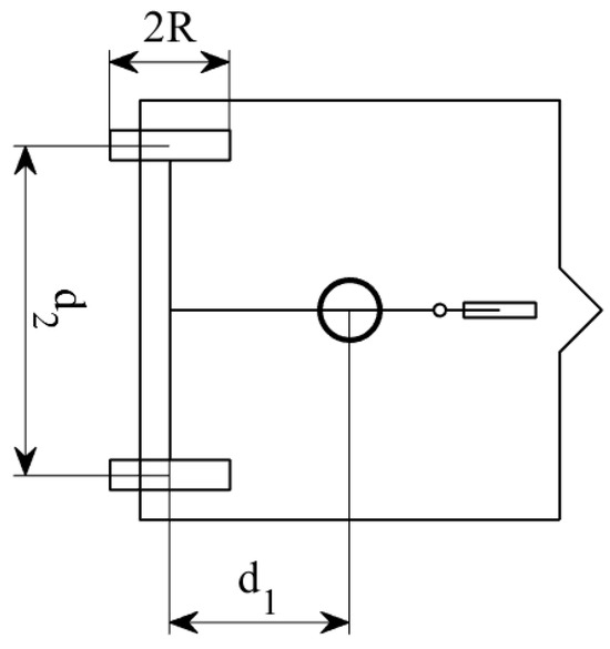
Figure 1.
The structure of MOBY robot. The actuated wheels have radius R and the distance between the wheels is . The vertical axis of rotation is located at a distance from the axis of the wheels.
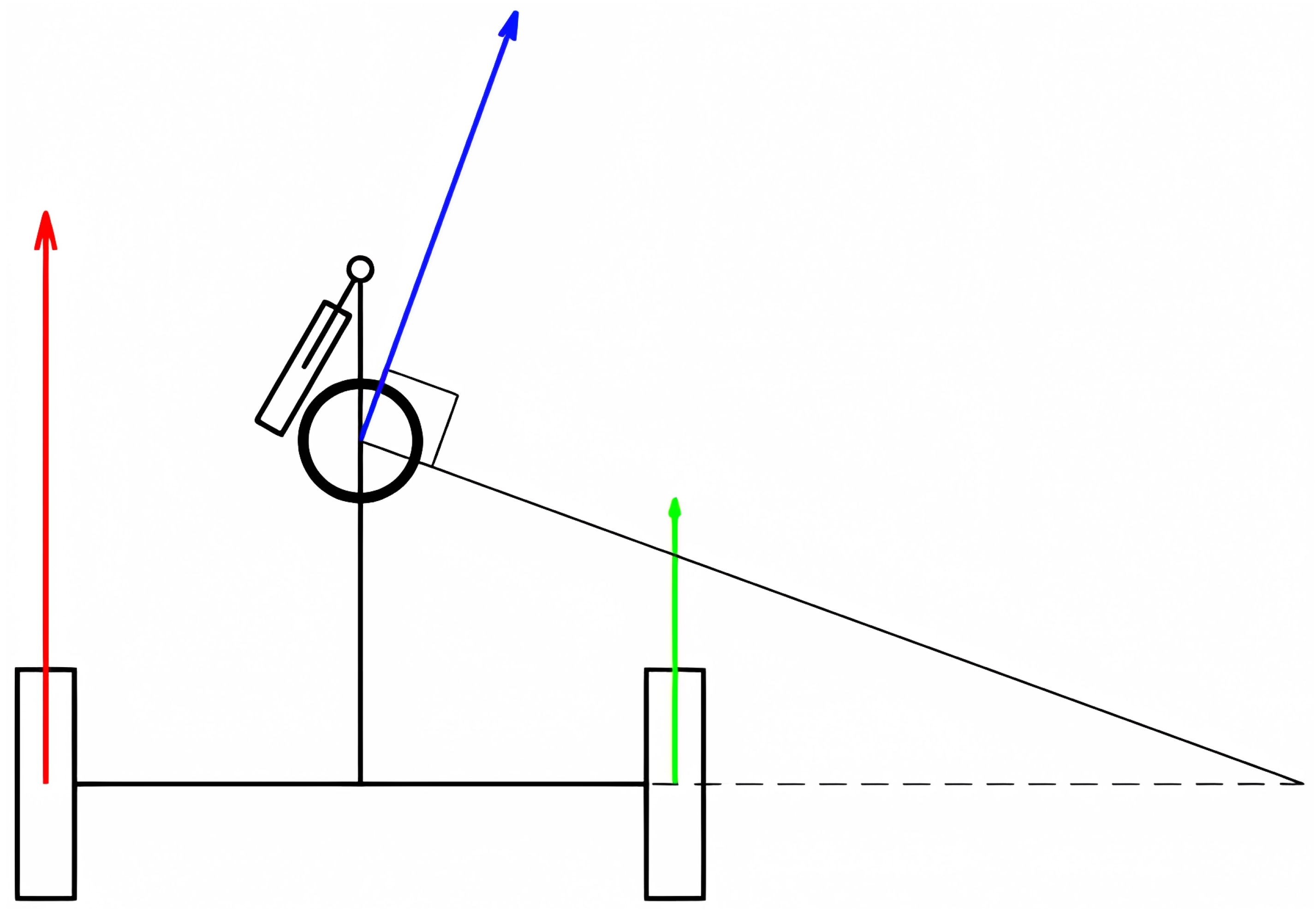
For the differential robot motion, the instant center of rotation is always found on the line of the axes of the wheels, as shown in Figure 2. The third vertical axis of MOBY allows for the orientation of this line arbitrarily while keeping an independent orientation on the body of the robot. A caster wheel is also mounted to the base of the robot for stability.

Figure 2.
The instant velocity of the center of the robot (in blue) is a function of the velocities of the wheels (in red and green).
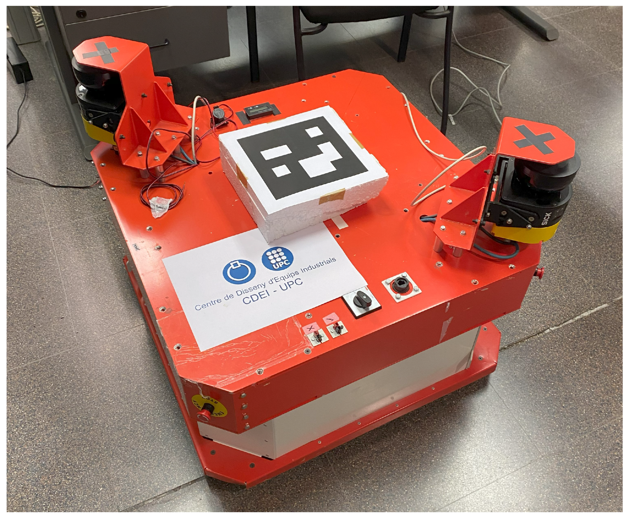
This simple kinematic structure was implemented in the MOBY robot that can be seen in Figure 3. It is important to notice that it is very simple to modify the type of wheels and the type of platform to adapt this robot to indoor or outdoor applications, as shown in the figure.

Figure 3.
The real robot used for this study’s experiments, MOBY.
The robot’s movement is controlled using platform velocity commands (three degrees of freedom in the plane) that are translated into velocity commands for each axis of the robot. In a code written in the C language, the commands for each axis are calculated based on the movement requirements. These data are sent to the robot every 4 ms using the UDP protocol. The robot is equipped with a PLC (programmable logic controller) that translates the velocity values for each axis into commands for the drivers of each motor to execute the requested movement. To follow a specific trajectory, the required velocity is calculated for each moment, and by integrating it, the position and orientation of the robot are determined.
3. Kinematic Analysis
A kinematic analysis of this type of robot can also be found in [9,11]. In the current work, we took a very similar approach, adapting it to the particular geometry of the MOBY platform and adding the caster wheel and fork.
Let us consider the active wheels of the robot as subjected to the no-slip condition to simplify the initial analysis. We defined the chassis as the differential wheels with their common axis and the structure that connects it to the platform.
The following generalized velocities describe the controlled velocities of MOBY:
- The angular velocity of the right wheel, , denoting the angular position of the right wheel as .
- The angular velocity of the left wheel, , denoting as its angular position from a reference.
- The angular velocity of the platform about the vertical axis, , with respect to the chassis, with an angular position of the platform with respect to the chassis .
Additionally, the following parameters, generalized coordinates, and velocities are used to describe its kinematics:
- The position vector of the center of the robot with respect to a fixed frame, , and its derivative .
- The angular position of the platform with respect to the fixed frame, , and its corresponding angular velocity, .
- The angular position of the chassis with respect to the fixed frame, , and its derivative .
- The radius of the actuated wheels, R.
- The distance between the rotation axis of the actuated wheels and the vertical rotation axis, .
- The distance between the actuated wheels, .
Notice that, with the definitions of these variables, the actuated rotation can be expressed as a function of and , as shown in Figure 4:
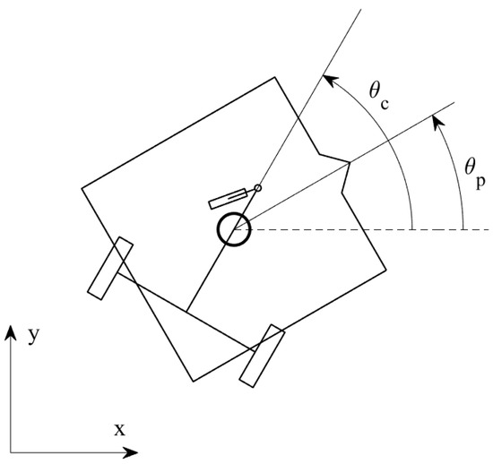
Figure 4.
The orientation of the robot as a function of the defined variables.
The wheels of the MOBY platform are standard fixed wheels, which impose the following constraints on the motion of the robot:
A third constraint transmits the angular velocity of the platform motor from the chassis to the platform,
enforcing Equation (1). When the relation in Equation (10) is applied to Equation (4), the constraint can be rewritten as
to explicitly show the relation between and the actuated variables of the system.
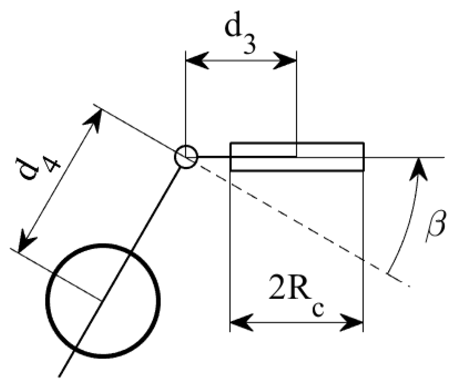
To take the dynamic effects of the caster wheel assembly into account, additional variables have to be detailed, which are shown in Figure 5:

Figure 5.
Variables defining the dimensions and configuration of the caster wheel assembly.
- The distance from the center of the platform to the joint of the caster fork, .
- The length of the caster fork from its joint to the axis of the caster wheel, .
- The radius of the caster wheel, .
- The angle of the caster fork with respect to the chassis, .
- The rotational velocity of the caster wheel, .
These variables also allow for the non-holonomic constraints of the caster wheel assembly to be applied as described in the work of Siegwart & Nourbakhsh [19]. The fourth constraint dictates the velocity of the caster fork as a function of the velocity and configuration of the robot. The fifth and final constraint imposes the no-slip condition on the caster wheel:
and
3.1. Forward Kinematics
The Jacobian matrix was used to model the relation between the three motors of the robot and its twist relative to the fixed frame of reference. Consider the twist of the platform with respect to the fixed frame. Then, the Jacobian matrix satisfies the following equation:
The wheel constraints in Equations (2) and (3), together with the relations among the orientation of the chassis, platform, and vertical degree of freedom in Equation (5), form the Jacobian matrix:
When the no-slip condition was applied, it was observed that the orientation of the chassis is a function of the position of the wheels:
where is the initial orientation of the chassis, and the initial values of and are set to zero.
3.2. Inverse Kinematics
For the inverse kinematics, the desired relation is
In the above expression, is the inverse of the previously computed Jacobian matrix, and it can be calculated to obtain the matrix:
3.3. Passive Degrees of Freedom
To integrate the response of the caster assembly with the velocities of the other degrees of freedom of the robot, the Jacobian matrix was augmented, adding two rows to . To produce this augmented Jacobian matrix, Equations (6) and (7) must be expressed in terms of the variables , , and . From the rewritten expressions, and were isolated, and the derivatives of their definitions were incorporated into the augmented Jacobian matrix, .
The augmented Jacobian matrix provides the expected values of the velocities and :
Notice that this Jacobian matrix is not square and, thus, is no longer invertible. The augmented inverse Jacobian matrix was obtained by repeating the previous process, this time using as a starting point and expressing Equations (6) and (7) in terms of the task space variables: , , and . The resulting matrix, , satisfies Equation (15), which produces the response of all the degrees of freedom of the system to a velocity command expressed in the task space:
with
4. Kinematic Behavior
Most of the non-intuitive behavior of this type of robot is due to the arrangement of the degrees of freedom of the robot and the kinematic constraints imposed on the system. The preferred driving strategy for uneven and rough terrains, which we call the pulling strategy, turned out to be unstable, and hence, it needed to be studied in detail. The control of the offset-differential robot is equivalent in terms of its kinematics to that of the look-ahead strategy of differential robots, which are widely used.
4.1. Driving Stability
As mentioned, the main phenomenon of interest was the instability described by Yun & Yamamoto [13] that appears when the machine is commanded to move with its actuated wheels in front, that is, with the wheels pulling the chassis, rather than pushing it. In the cited analysis, the authors derived the state space and the feedback control with input–output linearization for the look-ahead strategy. They showed that the internal dynamics exhibited instability when driving backwards, that is, when the tracking point was behind the driving wheels.
In order to show the instability, they used the equations of the internal dynamics when the reference point is moving and the robot is driving in a straight line, and they applied the Lyapunov function of the angular position of the wheels; see the referenced work for more details.
Yun and Yamamoto found that the robot has two equilibrium points. When applied to the offset differential robot, the first equilibrium point is the configuration in which the center of the robot and the midpoint of the axis of the active wheels are aligned in the direction of motion, with the wheels behind the center of the robot. This state can be called pure push, and it is a stable equilibrium point. If the robot is commanded to move in a straight line, it will gradually reach this state.
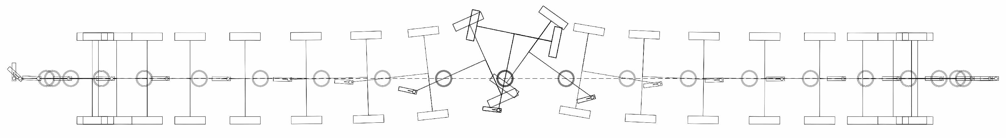
Unlike the first equilibrium point, the second equilibrium point is unstable. In this state, the wheels are ahead of the center of the robot. This unstable state can be called pure pull. With minimal disturbance, the angle between the chassis and the direction of motion will grow until they are perpendicular; at that point, the robot will start pushing and eventually reach the pure pushstate, as shown in Figure 6.
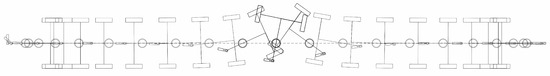
Figure 6.
Simulation showing the reversal of the direction of the chassis. From left to right, the robot accelerates backwards, holds its speed, switches from pull to push, and comes to a stop.
4.2. Kinematic Behavior
An easy solution is to avoid driving from this unstable equilibrium point; however, for rough and uneven terrains, such as agricultural ground, the pulling maneuver is advantageous. One easy way to see this is to consider the situation in which the robot has to climb a small obstacle with the caster wheel in front, which will create a jamming effect, as opposed to climbing with the active wheels in front.
Mathematically, the push–pull region of the velocity can be determined using the dot product of the current velocity and the direction of neutral steering. Assuming that the robot has a velocity of magnitude greater than zero, the cosine of in Equation (17) will be positive when the velocity is in the push region, negative in the pull region, and zero in the specific case of neutral steering. The particular cases of pure push and pure pull will yield 1 and −1, respectively.
The name neutral steering was given to the two particular velocities perpendicular to pure push–pull. These directions are of special interest since they present the tightest possible continuous turn radius achievable without alternating regions. During such a turn, the instant center of rotation of the chassis will be located at the midpoint between the two actuated wheels. This will result in their velocities having the same magnitude but opposite directions:
where
The speed at which the chassis approaches the pure push state when moving continuously in the positive x direction can be identified through the relations defined by the inverse kinematics and the derivative of Equation (10). The wheel speeds and , expressed in terms of and , are substituted in the velocity of the chassis:
Assuming a situation in which the robot is reversing in a straight line, a more general case can be obtained, expressing the desired velocity in a frame of reference aligned with the chassis:
where is the angle between the pure push direction and the direction of the desired velocity, and c is the magnitude of the velocity of the robot. Note that both sides of the expression can be divided by c, yielding
which details the instant turn radius of the robot during the reversal. This points to the trajectory being independent of the magnitude of the velocity.
If the robot is going in a straight line, would ideally be zero. Assuming is fixed and c is decided via the operator, the only way to influence is by changing the angle between the chassis frame of reference and the desired velocity. Taking advantage of this, the velocity vector may simply be rotated so that it is aligned with the chassis’s frame of reference. This would stop the progress of the reversal. However, considering Equation (20), when the robot is in the push region with the same value of c, it is evident that the rate at which the spontaneous turn of the chassis accelerates is the same as that at which it slows down when approaching pure push. Using this knowledge, it becomes clear that there are velocities that can not only halt the progress of the turn but also reverse it. Therefore, it can be inferred that there is a value of that yields the opposite to the current value of .
Considering only cases in the pull region, , the direction that corrects the attitude of the chassis is . Thus, to rectify the orientation of the chassis, the velocity is mirrored along the x-axis of the chassis’s frame of reference.
Because the correction is prescribed through modifying the task space velocities, it leads to inaccuracies in the trajectory. Ways of mitigating the error between the corrected and planned trajectories are discussed in the following section.
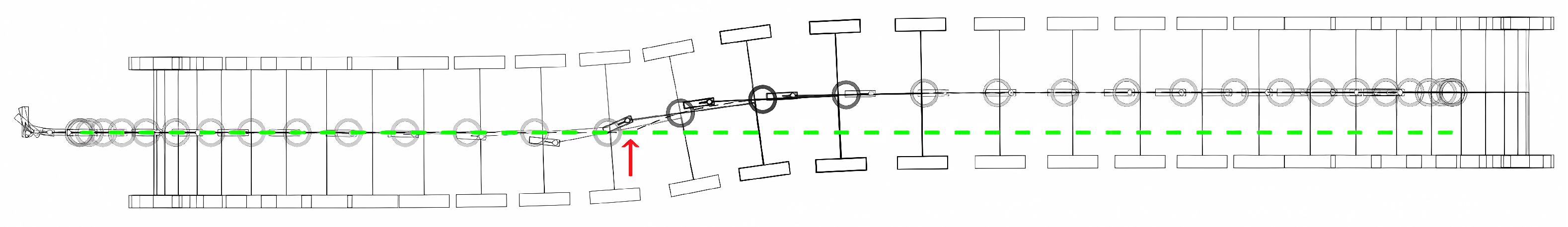
The earlier the tendency to switch the chassis is corrected, the smaller the change in trajectory. If the trend to push is continuously corrected, it will not proliferate, provided that there are no significant unexpected forces involved. This was not the case in the simulation shown in Figure 7, in which was allowed to grow freely from the beginning of the motion to the point shown with the red arrow.
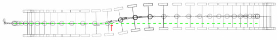
Figure 7.
The corrected motion of the chassis when reversing. The red arrow shows the point in the trajectory (the dashed black line) where the correction starts being applied. The dashed green line shows the originally intended trajectory.
This approach can be extended to any trajectory by matching to the instant angular velocity of the chassis. This generalization requires the introduction of an additional variable, , which is the angle of the velocity with respect to the chassis when the robot is moving in a circular trajectory. It can be found using the relation
where is the angular velocity of the robot with respect to its instant center of rotation (positive is counter-clockwise). The corrected velocity vector is produced by mirroring the input velocity along an axis passing through the center of the robot with the angle with respect to the input velocity.
The chosen approach, to mirror the direction of the velocity without changing its magnitude, returns the chassis to its target orientation at the same rate at which it left it, assuming that the change of region was purely kinematic. If the disturbance that initiated the reversal was dynamic in nature, the maximum torque that the motors can provide may prevent the robot from matching the growth in angular velocity. In that case, the robot will return to the desired configuration as rapidly as the motors allow, attempting to maintain the target speed.
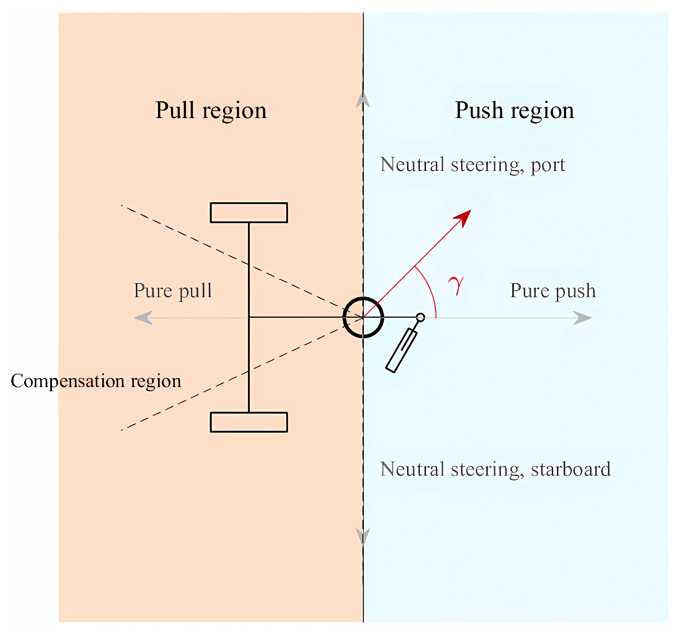
To avoid returning to the pull region unnecessarily, a compensation regionis defined, beyond which the compensation algorithm is not applied. The compensation region is unlike the other regions in the sense that its bounds can be set arbitrarily and change during motion. For instance, if a loss of traction on the wheels or tipping over are concerns, the compensation region may change, depending on the velocity of the robot. An example of a possible compensation region can be seen in Figure 8.
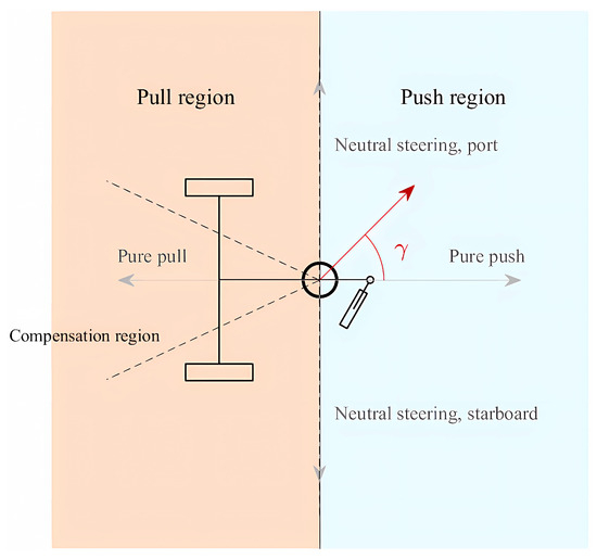
Figure 8.
Regions and main directions of the robot. The compensation region is defined by the user and can even include part of the push region. The dark red arrow shows an example of a velocity in the push region.
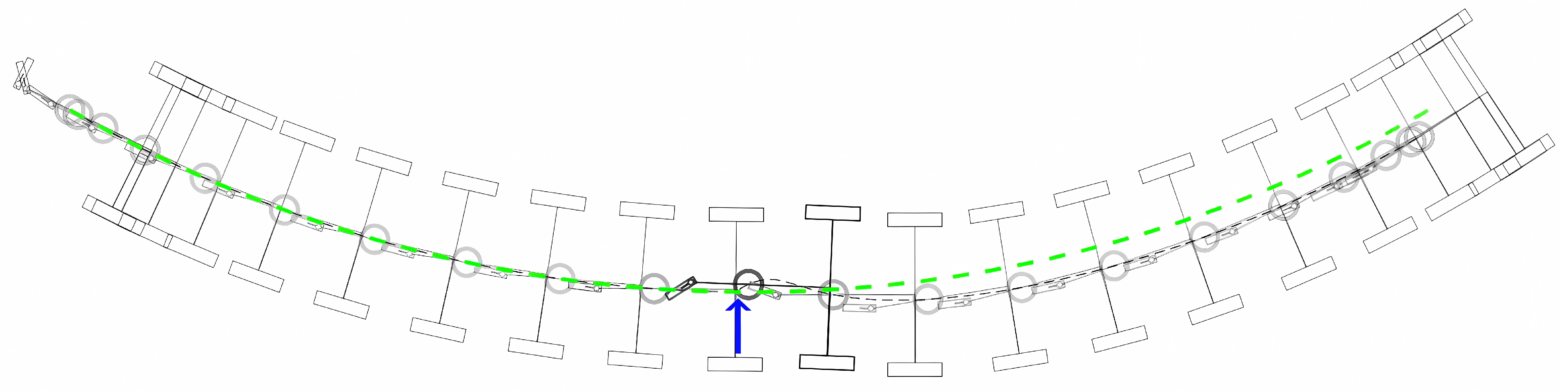
To better observe the compensation algorithm in action, the simulation shown in Figure 9 introduced unanticipated forces in the shape of blows to the fork of the caster wheel. In the following simulation, the impact was simulated as a 4000 N force acting on the fork of the caster wheel for 25 ms. The direction of the force was perpendicular to the chassis and roughly towards the center of rotation.
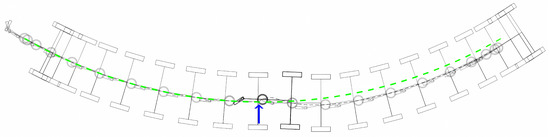
Figure 9.
Dynamic simulation of the response of the robot to an impact on the fork of the caster wheel. The blue arrow indicates the position of the center of the robot when the force is applied and its direction. The green dashed line shows the expected trajectory had there been no impact.
As can be seen in Figure 9, the compensation only returns the chassis to the predetermined orientation. This is enough to prevent the spontaneous change of region, but getting the robot to go back to the path requires a recalculation of the trajectory to accommodate the merging back into the original path.
Looking further into Equation (23) and introducing a definition for , which is the difference of and , reveals that the same effect may be achieved by rotating the input velocity vector two times, the opposite of . Note that, while the results of Equations (23) and (24) are the same, the transformations are not equivalent.
A more general expression can be written as shown in Equation (25), in which k determines the aggressiveness of the compensation, ranging from 0 (no compensation at all) through to 1 (only stopping the progress of the switch but not returning to the desired configuration) and then returning to the desired configuration faster with a higher value of k. The compensation region should be smaller with a higher value of k to avoid ineffective compensation.
5. Driving Strategy
The insight gained from the kinematic analysis was used to design maneuvers so that the robot would be in the pull region for extended periods of time. In order to avoid a region change, two rules emerged from the previous sections:
- The trajectory must be smooth, that is, it must be continuous as well as continuously differentiable. This extends to the initial position of the robot. The vector analogous to the pure pull direction must be tangent to the velocity at the starting point; otherwise, significant compensation will be necessary to remain in the pull region over the long term. If the first part of the path is curved, and should be equal.
- Turns with a radius smaller than are possible but should be avoided. While momentarily turning tightly does not guarantee a change in velocity region, sustained rotation with such a small radius will eventually result in a change in the direction of the chassis.
In addition to disturbances due to the terrain, instability manifests inherently due to the fact that commands cannot be given to the motors in a perfectly continuous manner. Every slight change in the desired turn radius will result in a small lateral shift, even if and were equal in the previous instant. The lower the refresh rate and the more sudden the change in turn radius, the more deviation to be expected. For this reason, the trajectory should be recalculated periodically to adapt to changes brought on via compensations during motion. The more important the accuracy is to the particular application, the more often trajectories should be amended to redress the lateral deviation caused by the compensation algorithm. These recalculations may concern only a small part of the path and lead the robot to rejoin the original route or entail the recomputation of the entire motion.
General trajectories with a changing curvature will always exhibit unstable behavior, even in smooth, continuous motion. One easy way of defining a viable trajectory involves concatenating a series of arcs that are tangent to each other at the points where they meet. In this case, the first arc would need to be tangent to the direction of the robot at its starting point.
An interesting characteristic of the motion is that the progress of the switch in chassis orientation is independent of the velocity, as evidenced by Equation (21). This means that, absent any dynamic effects, the trajectories that are consistent with the first two rules can be executed at any speed allowed by the actuators.
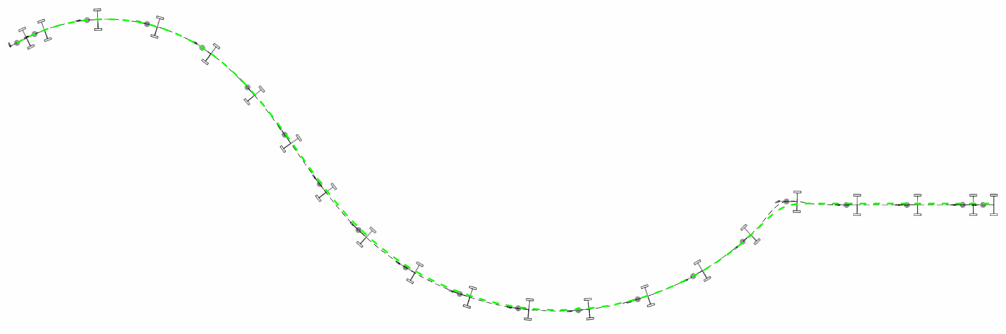
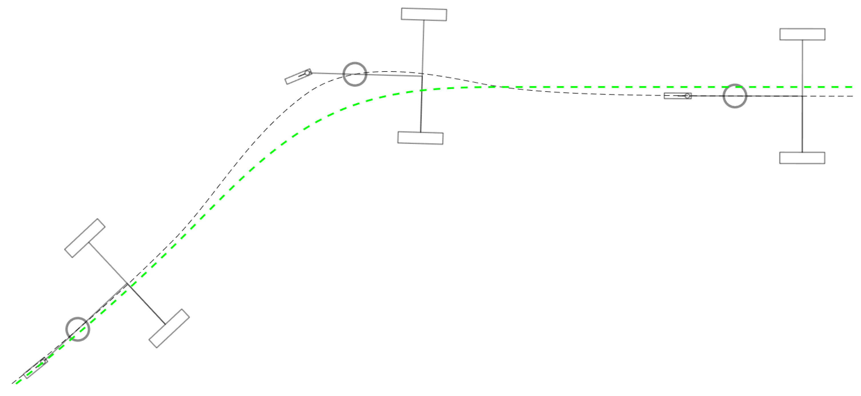
Another kinematically viable strategy is to always keep the instant center of rotation on the axis of the actuated wheels of the previous instant. This is also accomplished by building a trajectory of concatenating arcs, as shown in Figure 10. This time, there is a discontinuity in the velocity each time the robot passes from one arc to the next. Instead, what is kept track of is the orientation of the chassis, and the direction of the center and radius of the turn are calculated so that and remain equal during the motion, absent any disturbances, see detail in Figure 11. This method solves the otherwise inherent need to compensate every time the radius of the turn of the trajectory changes at the cost of decreased maneuverability. Additionally, if the instant radius changes too suddenly, it will result in large on-the-spot wheel velocity variations. Such changes not only lead to spikes in the needed torque but may also cause the friction force between the tires and the ground to exceed the static friction threshold and slide. One final disadvantage of this method is that it only deals with the kinematic causes of the error of , meaning that other sources, such as external forces, remain.

Figure 10.
The trajectory determined by concatenating arcs and a straight line. The dashed green line is the pre-defined trajectory. The path begins with a 60° arc with a radius of 5 m; then, it applies a 90° arc with a radius of 8 m and finally a 5-m-long straight line. The angular velocity changes uniformly in the stretches between arcs. The shapes of the chassis and the wheels of the robot show the position and orientation of the robot at evenly spaced instants.
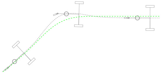
Figure 11.
Detail of the previous figure showing how tighter turns are prone to causing an increase in position error due to the discrete nature of the velocity commands.
6. Dynamic Behavior
6.1. Lateral Stability
We denote lateral stability as the property of the robot that avoids the loss of contact on its wheels and rolling over, thus impeding its locomotion. For a study of the stability of mobile robots, see, for instance [20]. For low velocities, when dynamic effects can be neglected, a quasi-static analysis is used.
The presented implementation of the offset-differential robot has three points of contact with the ground, thanks to the caster wheel. Because its velocity in the selected applications (rough and uneven terrain) is low, this is the case we studied in this work. However, checking the stability under dynamic conditions would be an interesting extension of this work.
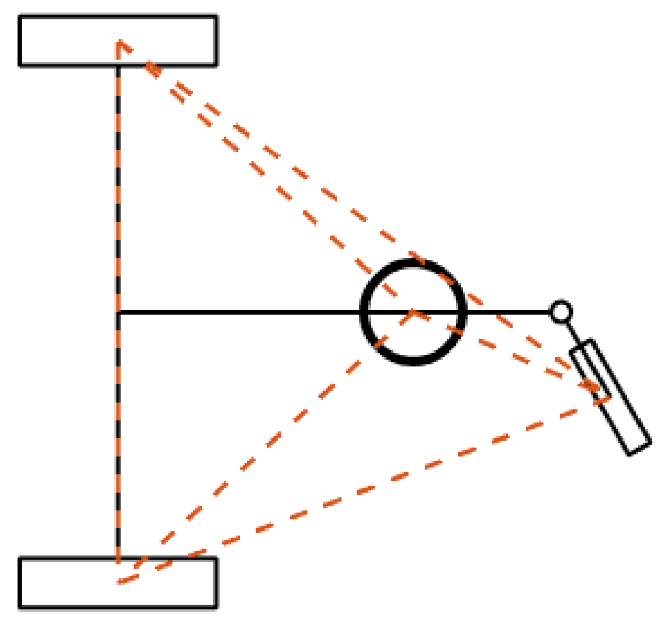
The tip-over stability margin was computed with a simple static analysis, considering the center of inertia, the angle of the contact plane formed by the three contact points, and the reaction forces at the wheels. In the case of the three-wheeled robot, we can create tip-over planes by joining the contact point of two wheels with the center of inertia of the robot, forming a tetrahedron; see Figure 12.
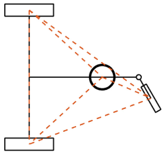
Figure 12.
The stability tetrahedron is formed by the contact points of the wheels and the center of inertia of the robot.
In order to ensure static stability, the axis of the weight force, located at the center of inertia, must fall within the tetrahedron in order to determine whether the robot will roll over.
It is easy to see that, for the offset-differential robot, unless the load is perfectly centered at the vertical rotation axis, lateral stability must be checked during the motion planning of the robot, even in smooth, horizontal terrain. The angle of the caster wheel needs to be known in order to perform this check. As we will see later, being able to sense the heading angle of the caster wheel is important for the accurate control of this robot.
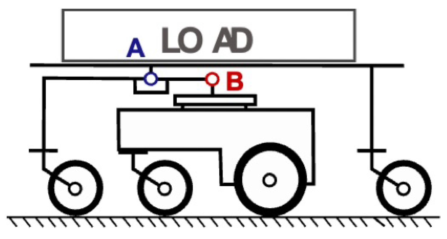
Greater stability can be accomplished for this robot using an additional structure that does not change the kinematic behavior. It consists of additional caster wheels connected to the robot via an additional mechanism that allows continuous contact with the surface and load distribution among the wheels. A schematic representation can be found in Figure 13. Joints A and B can be either cylindrical or Cardan joints, depending on the terrain’s irregularity. The distance between joints A and B determines the normal reaction on the drive wheels.
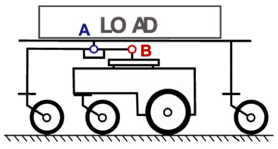
Figure 13.
A solution to increase lateral stability without changing the kinematic behavior.
6.2. Dynamic Model
The dynamics of the offset-differential robot were modeled using the Lagrangian formulation. To do so, a few more variables were defined:
- The mass, , and the moment of inertia, , of the chassis (excluding the actuated wheels).
- The mass, , and the moments of inertia, , of the actuated wheels, which were assumed to be the same for both.
- –
- is the moment of inertia of the wheel spinning through its axis.
- –
- is the moment of inertia as it relates to the contribution of the wheel when the whole chassis is rotating. It was calculated as the moment of inertia of the wheel spinning about its radius plus the additional inertia brought about by the distance from the center of rotation of the chassis, which is taken into account through the parallel axis theorem.
- The mass, , and the moment of inertia, , of the platform.
- The mass, , and the moment of inertia, , of the caster fork.
- The mass, , and the moments of inertia, and , of the caster wheel.
The distance between the centers of mass of the actuated wheels was considered the same as the distance between the centers of their tires, .
The present case involves the robot moving on flat, even ground, which makes the potential energy term of the Lagrangian formulation null.
The mass matrix of the system, M, was calculated using the definition of the kinetic energy of the bodies, as in [11]. The Coriolis matrix, C, was calculated using the Christoffel symbols of the first kind method [21]. The five constraints applied to the robot were written as Pfaffian constraints [22], such that:
Here, is a 5-by-8 constraints Jacobian, and q is a vector containing the degrees of freedom of the system. q can be divided between active, , and passive, , variables. These vectors come together to form q, the 8-by-1 vector that contains all the variables in the order . This leads to Equation (27):
where is a vector containing the Lagrange multipliers.
6.3. Forward Dynamics
Using Equation (27), the forward dynamics is easily solved.
Note that in the previous expression, the general force term was replaced by a term containing the torque supplied by the three motors, , and a term outlining the dynamic contribution of friction on all the joints affected by it, . An additional force vector, , was also included in order to introduce external forces on any of the degrees of freedom. This includes torques on the actuated wheels, platform, and caster wheel assembly, as well as forces applied directly in the x and y directions on the center of the robot.
6.4. Inverse Dynamics
As shown in [11], the calculation of the Lagrange multipliers can be conveniently bypassed in the inverse dynamics. Considering the nature of ,
the dynamic equilibrium equation can be rewritten as shown in Equation (30).
In the previous equation, is the input tensor that maps the control variables, u, to the coordinates of the system [23]. Note that the external forces in Equation (30) include only those that can be anticipated.
In the simulations, the friction on the joints of the robot is approximated using a viscous friction model:
7. Tests
To verify the dynamic model, as well as to demonstrate the benefits of applying the compensation, two simulations and two experiments were conducted. Both simulated similar motions, comparing compensated and uncompensated versions of each. In the case of the simulations, an additional test was performed to quantify the impact of the caster wheel on the dynamics of the system.
7.1. Simulations
The dynamic model of the robot was used to understand the impact of the kinematic instability of the robot on the torque needed to comply with the velocity commands. In addition, the modeling of the caster wheel also allowed for the analysis of its own contribution to the system.
Two simulations were carried out to these ends using the mass properties presented in [10] for comparison. Both started with the chassis of the robot anti-parallel to x and an angle of . For the first simulation, the instability was allowed to progress freely. The second run applied the compensation algorithm since the beginning of the movement. The raw velocity commands were the same for both, constantly accelerating during the first quarter of the simulations, holding a velocity of m/s and decelerating at the same rate during the final part. The configuration of the robot during the first test can be seen in Figure 6.
For clarity, the simulations were conducted without viscous friction at the joints. The simulated total mass of the robot was around 130 kg, including kg of the caster fork and kg of the caster wheel. The moment of inertia of the chassis was . In addition, the moments of inertia of the actuated wheels and the components of the caster wheel were also considered for all directions in which they rotated.
In all simulations, the refreshing rate of the engines was 1000 Hz, as was the refreshing rate of the dynamics calculations. The time-integration scheme used to produce the trajectories was the forward Euler method.
Tests were carried out in MATLAB using an i7-10750H CPU and 16 GB of RAM. The chosen time step size was 1 ms.
7.2. Experiments
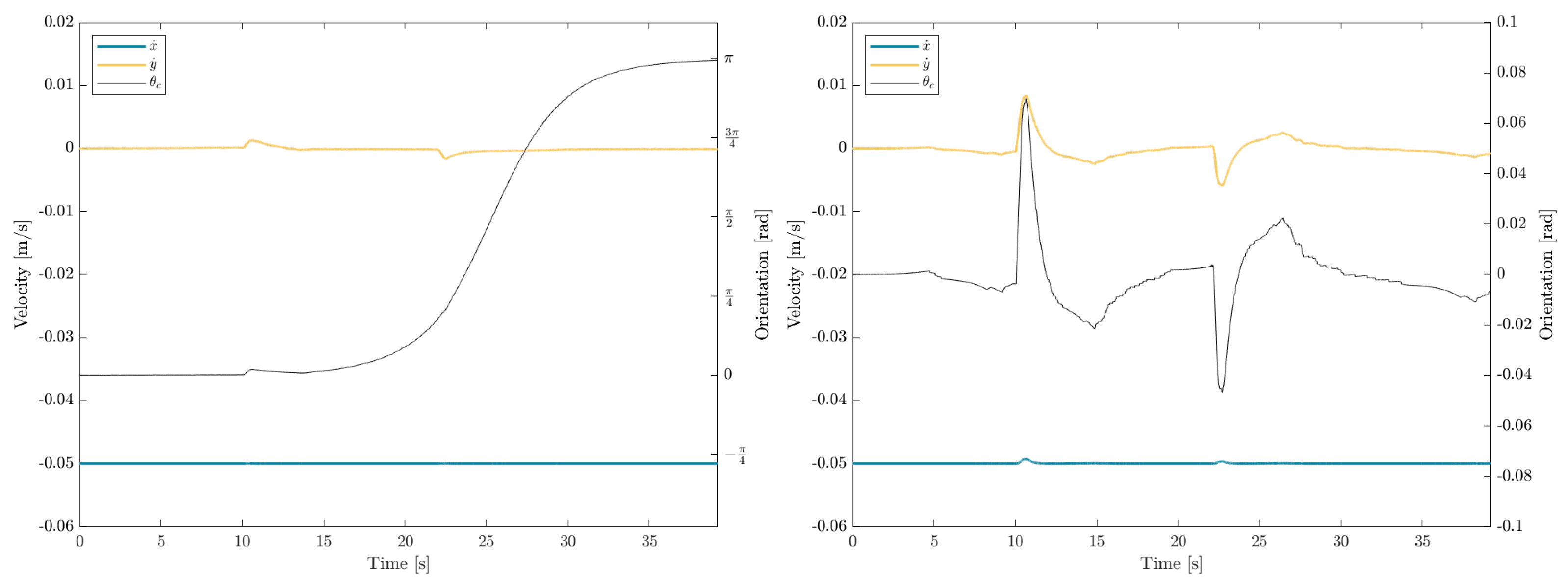
Two experiments were conducted with the real omnidirectional robot depicted in Figure 3. The robot was ordered to move forward 2 m and then back. By doing so, it was ensured that the return half of the itinerary began in the pull region. During the journey back to its starting point, the robot was “hit” with two impulses of alternating directions. These simulated impacts were short-velocity commands perpendicular to the motion of the robot.
In the first test, the robot was allowed to react naturally. In the second test, the compensation algorithm was implemented so that the robot could recover its original chassis orientation.
The distance between the center of the robot and the wheel axis in Figure 1 in the case of the real robot was m. Commands were given to the real robot once every 4 ms.
7.3. Uncompensated Pull-Region Motion
The robot was ordered to move forward 2 m at a velocity of m/s. Then, the velocity was reversed. After 10 s, an order was given to add a perpendicular component of m/s to the velocity during 0.4 s; 22 s into the reverse motion, the same order was given but towards the opposite side.
7.4. Compensated Pull-Region Motion
The previous experiment was repeated, this time with the compensation on. In addition, the duration of the “hits” was doubled to allow the perpendicular velocity to grow more than it had in the previous test.
8. Results
8.1. Simulations
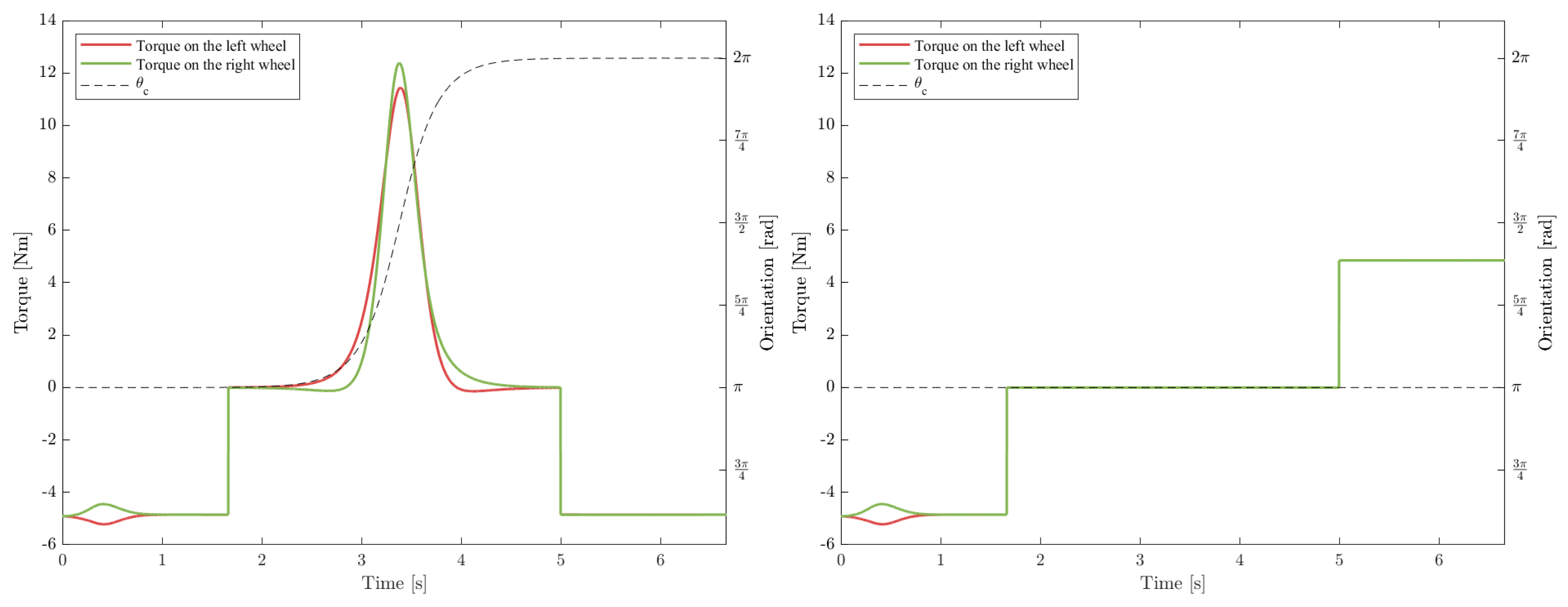
During the switch shown in Figure 6, the robot had to quickly alter the velocity of its motors to maintain the velocity of the center. To do so, high torque needed to be supplied to the actuated wheels, as can be seen in the left graph of Figure 14. Also note that, in addition to the effect of the caster wheel, the torque profile was the same when accelerating and slowing down. This was due to the chassis rotating 180° through the second stage of motion.
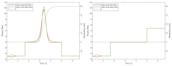
Figure 14.
The torque required on the actuated wheels to perform the motion in Figure 6. (Left), uncompensated; (right), applying the compensation every instant.
When correcting the rotation of the chassis, the torques were those presented in the right graph of Figure 14. The three phases of motion were plainly visible: acceleration, holding m/s, and coming to a stop.
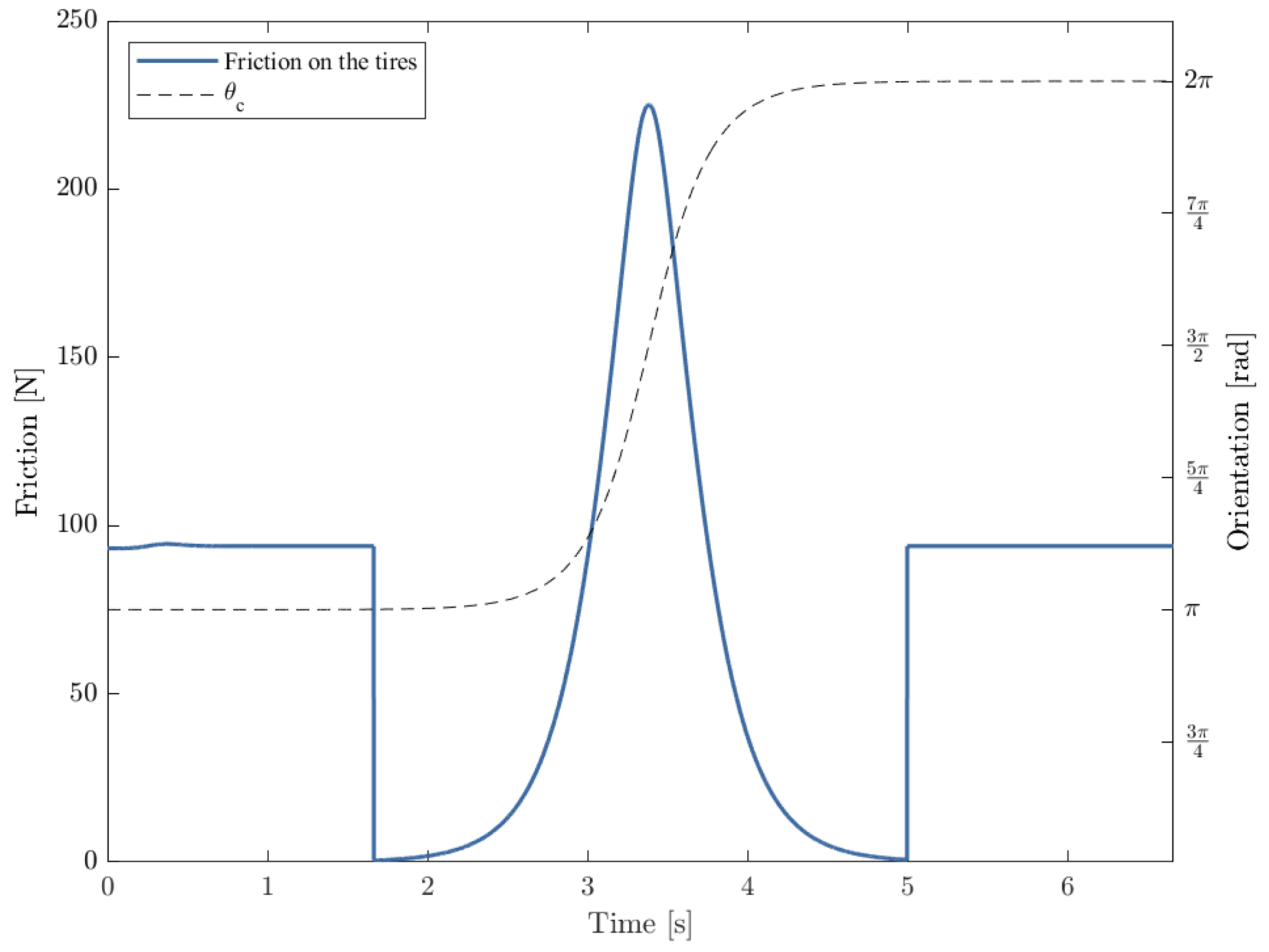
In the first simulation, the highest torque required for any of the wheels was Nm, whereas the same value for the second simulation was Nm. In addition, the combined friction with the ground needed for all three wheels to execute the motion, shown in Figure 15, was much greater in the first run, reaching 225.1 N. Had there been no reversal, the maximum necessary static friction would have been 94.5 N.
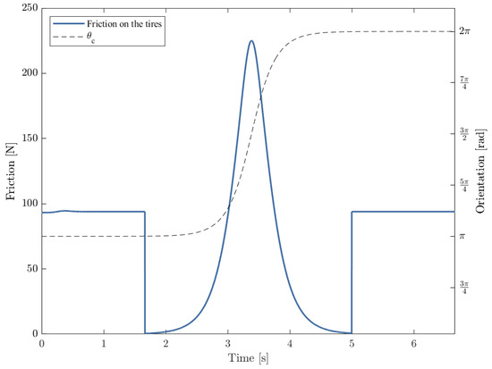
Figure 15.
The magnitude of the friction with the ground needed for the robot to perform the motion in Figure 6.
This points to another issue as a consequence of instability: the fact that the required force between the ground and tires may exceed the maximum stiction.
The caster wheel presented instability in some ways analogous to the offset differential drive, the main difference being that it was not active. As such, what dictated its behavior was the movement of the point in the chassis connected to the caster fork with a revolute joint. This motion, through the constraints defined in Equations (6) and (7), informed the response of the constrained degrees of freedom and .
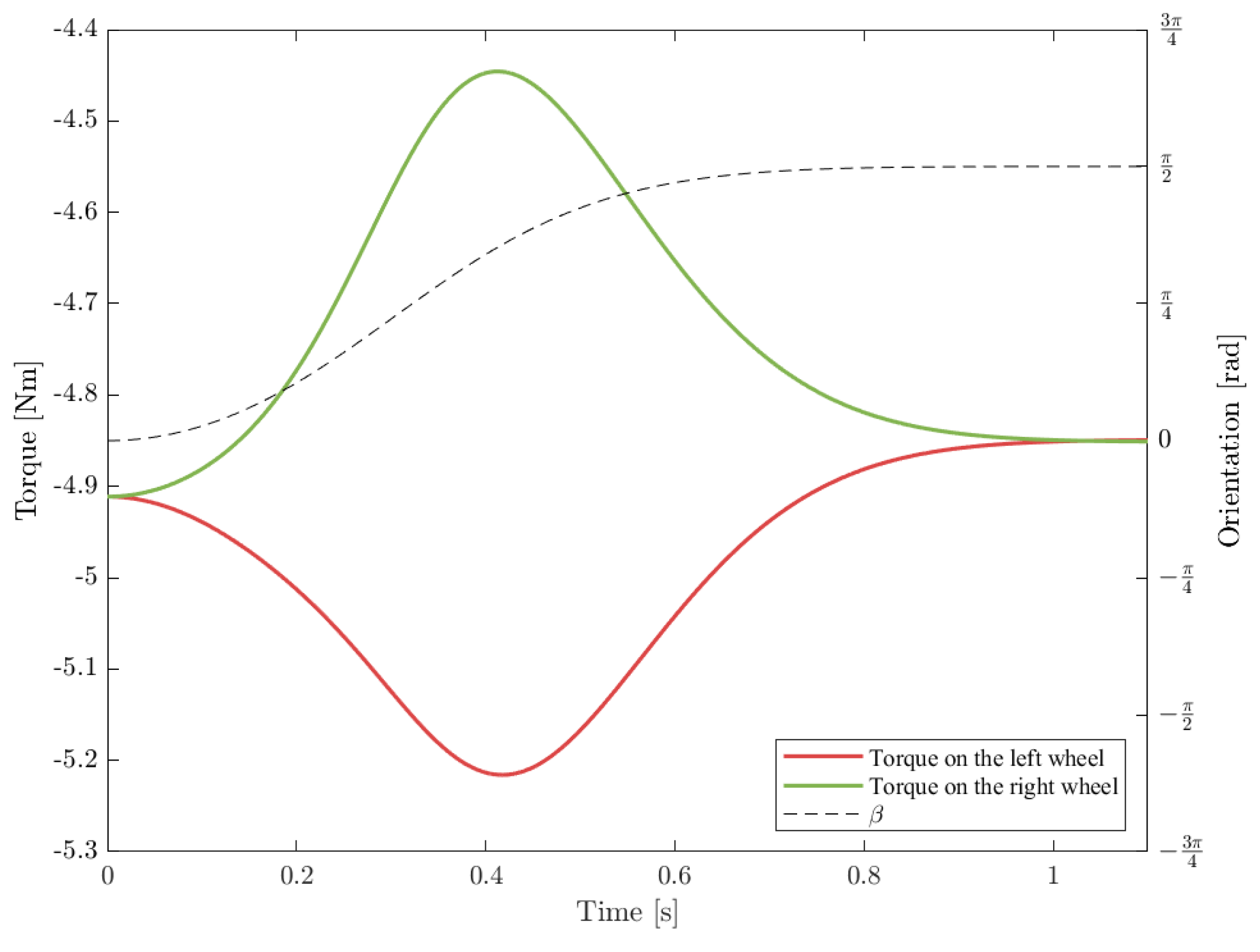
In the case of the previous simulations, the low velocity of the robot at the beginning of the motion meant that the torques that the motors needed to produce to make up for the increased resistance due to the position of the caster wheel were relatively low, as shown in Figure 16.

Nonetheless, there are cases in which the caster wheel could have a greater impact on the dynamics of the whole system. An example is the common case in which the robot is moving in the pure push direction and then is ordered to move in the pure pull direction. The caster wheel is then in an unstable equilibrium with a value of . Granted that there are no notable disturbances, the robot can reach significant speeds while the caster wheel remains in or close to the unstable equilibrium point.
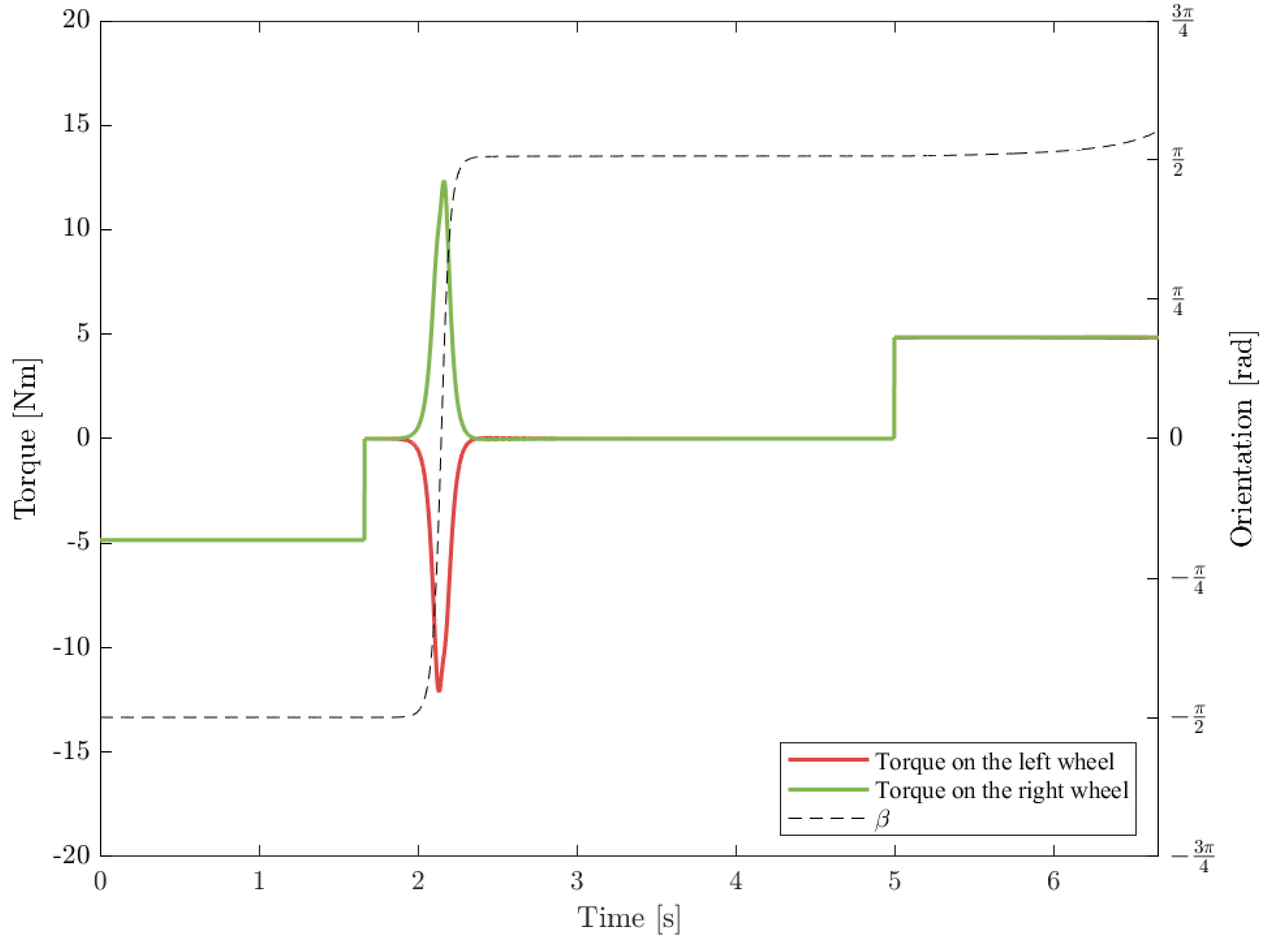
Despite being far less massive (with a 1.2 kg combined mass), the instability of the caster wheel assembly may have an impact on the torque needed by the wheels comparable to that of the whole chassis. In the situation described in Figure 17, the caster fork stayed at its unstable equilibrium point during the acceleration phase and suddenly came out of it during the constant-velocity stage. In this simulation, the peak torque was Nm, which was supplied to the right wheel.
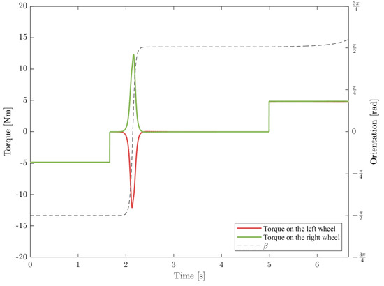
Figure 17.
Dynamic effects of the caster wheel when it exited its unstable position during the second phase of compensated motion.
Another important consequence of the dynamics of the caster wheel is its potential to initiate a region switch. As long as the velocity commands are discrete, the response of the motors to the rotation of the caster wheel is always slightly off. If left uncorrected, the deviation induced by the caster wheel has the potential to greatly accelerate the progress of the region switch.
All three simulations lasted 6.6 s. When the time needed to load the dynamic model and initialize the variables was not taken into account, the computation times for the simulations were 1.68 s for the first simulation, 2.05 s for the second, and 2.30 s for the third. Each of these times included the inverse and forward dynamics calculations of the whole simulation.
It is worth noting that there is still room for improvement when it comes to optimizing the simulations so that the results can be produced faster, should the need arise.
8.2. Experiments
As expected, the first disturbance was more than enough to initiate the turn shown in the left graph of Figure 18.
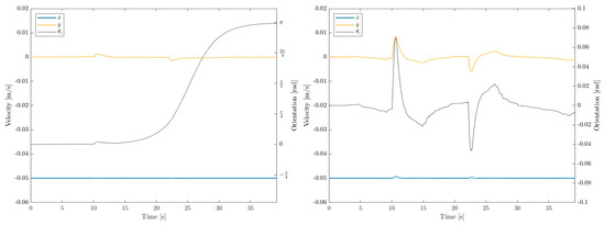
Figure 18.
Velocities and chassis angle during the experiments: (left), the first experiment; (right), the second experiment (with compensation). Note the difference in scale between the plots.
In the second run, the velocities of which are displayed in the right graph of Figure 18, the perpendicular velocities made the magnitude of increase as the robot was shoved. However, as soon as the disturbance ceased, the chassis quickly recovered its original heading.
9. Conclusions
In this work, the aim was to fully characterize the dynamics of the offset differential robot, especially its behavior in the unstable driving zone. While this region has been studied, and some of its advantages have been identified for non-omnidirectional, differential-drive robots, the use in the omnidirectional robots that present this feature has not been studied so far, to our knowledge.
With the results of the simulations, it became apparent that the reversal of the robot’s region of velocity is a phenomenon of kinematic origin that has dynamic consequences. The simulations also showed that the orientation of the caster wheel can be problematic in some instances. For this reason, for relatively high-speed applications, the caster wheel should be instrumented, and its orientation should be taken into account when trajectories are planned.
There are clear advantages to the use of the unstable pull region in the operation of offset differential drive robots, from simple increases in speed in certain situations to reductions in the risk of getting stuck while navigating difficult terrain. In the context of agricultural applications, advancing with the actuated wheels in front makes soft and irregular ground easier to traverse, not only on account of their larger diameter but also because they use the terrain to propel themselves and to compensate for the moment that may make the robot stuck on some terrain.
As shown in the simulations, the cost of allowing the robot to choose its velocity region freely can have detrimental effects on its odometry and the accuracy of its movement. Often, this would mean having to choose not only between precision and velocity but also safety since a loss of traction in the wheels could endanger the robot and its environment.
As a result of the instability inherent to the design, constant corrections are necessary to remain in the pull region. These corrections can be successfully applied using the methods described in this paper. These methods can be generalized to a broad range of trajectories, encompassing most situations. However, trajectories involving fast, tight turns and great variations in turning speed are susceptible to a noticeable position error. In these circumstances, there is still a decision to be made between speed and accuracy, but the risks of losing traction or not having the adequate capacity to supply the necessary torque to the wheels are similar to those faced with the robot in its pure pull (or equivalent) direction. If the robot is left unmonitored, there is the possibility of a region switch being caused at an unexpected point, greatly increasing the chance of failing to perform as required.
Finally, the dynamic effect of the caster wheel was considered, opening the door to torque control for the offset differential drive robot structure. The inclusion of the caster wheel assembly in the dynamic model proved especially relevant to understanding the way it can contribute to the convergence into the stable equilibrium of the robot by accelerating it. For an accurate calculation of torques, the orientation of the caster wheel may need to be known, for instance via an encoder.
The dynamic model can also serve as the basis for more research into issues that offset-differential machines may run into, like a loss of traction, tipping over when turning, driving up slopes, and getting wheels stuck in agricultural settings.
Future Research
The current model is to be used to create more accurate control strategies for offset-differential robots. With this goal, the model will be further refined by incorporating the inertia of the rotary actuation and transmission systems. In existing market solutions, the centers of inertia for both the actuation–transmission part and the upper platform parts of the robot are not completely aligned with the vertical axis of rotation. This results in additional dynamic effects causing alterations in the robot’s position during rapid movements. Studying these dynamic effects in detail is also important for implementing path planning and control strategies to mitigate their impact.
The dynamic effects of the orientation of the caster wheel on the computed torques make identifying this orientation necessary in order to obtain accurate torque commands. The intention is to equip the robot with a caster wheel featuring an encoder to constantly monitor its orientation in order to obtain better torque characterization and also a continuous computation of lateral stability.
The need for more precise and accurate mobile robots is also related to their applications in mobile manipulation. Exploration is underway for a joint solution involving a mobile platform and a robotic arm designed to function as a unified system with some shared axes. The goal is to have an omnidirectional manipulation system with the needed accuracy for interaction with the environment.
Author Contributions
Conceptualization, A.P.G. and C.D.-M.; methodology, A.P.G. and J.B.T.; software, J.B.T.; validation, C.D.-M. and J.B.T.; formal analysis, J.B.T.; writing—original draft, J.B.T.; writing—review and editing, A.P.G.; supervision, A.P.G. and C.D.-M. All authors have read and agreed to the published version of the manuscript.
Funding
This research was supported in part by award TED2021-131877B-I00 and the AgroMOBY project (PDR 2014-2022), award 56 30141 2021, from the Operació 01.02.01 de Transferència Tecnològica del Programa de desenvolupament rural de Catalunya 2014–2022. The contents are solely the authors’ responsibility.
Data Availability Statement
Data are contained within the article.
Conflicts of Interest
The authors declare no conflicts of interest.
References
- Prados Sesmero, C.; Buonocore, L.R.; Di Castro, M. Omnidirectional Robotic Platform for Surveillance of Particle Accelerator Environments with Limited Space Areas. Appl. Sci. 2021, 11, 6631. [Google Scholar] [CrossRef]
- Qian, J.; Zi, B.; Wang, D.; Ma, Y.; Zhang, D. The Design and Development of an Omni-Directional Mobile Robot Oriented to an Intelligent Manufacturing System. Sensors 2017, 17, 2073. [Google Scholar] [CrossRef] [PubMed]
- Jacobs, T. Omnidirectional Robot Undercarriages with Standard Wheels—A Survey. In Proceedings of the 25th IEEE International Conference on Mechatronics and Machine Vision in Practice (M2VIP), Stuttgart, Germany, 20–22 November 2018. [Google Scholar]
- Taheri, H.; Zhao, C. Omnidirectional mobile robots, mechanisms and navigation approaches. Mech. Mach. Theory 2020, 153, 103958. [Google Scholar] [CrossRef]
- Ramirez-Serrano, A.; Kuzyk, R. Modified Mecanum Wheels for Traversing Rough Terrains. In Proceedings of the 2010 Sixth International Conference on Autonomic and Autonomous Systems, Cancun, Mexico, 7–13 March 2010; pp. 97–103. [Google Scholar] [CrossRef]
- Chung, W.; Moon, C.; Jung, C.; Jin, J. Design of the Dual Offset Active Caster Wheel for Holonomic Omni-directional Mobile Robots. Int. J. Adv. Robot. Syst. 2010, 7, 105–110. [Google Scholar]
- Nasu, S.; Wada, M. Mechanical Design of an Active-caster Robotic Drive with Dual-Wheel and Differential Mechanism. In Proceedings of the Annual Conference of the IEEE Industrial Electronics Society—IECON2015, Yokohama, Japan, 9–12 November 2015. [Google Scholar]
- You, Y.; Fan, Z.E.A. Design and Implementation of Mobile Manipulator System. In Proceedings of the International Conference on CYBER Technology in Automation, Control, and Intelligent Systems, Suzhou, China, 29 July–2 August 2019. [Google Scholar]
- Jung, M.J.; Shim, H.-S.; Kim, H.S.; Kim, J.H. The miniature omni-directional mobile robot OmniKity-I (OK-I). In Proceedings of the IEEE International Conference on Robotics and Automation 1999 (ICRA’99), Detroit, MI, USA, 10–15 May 1999. [Google Scholar]
- Giro Perez, P. Dynamic Modelling, Parameter Identification, and Motion Control of an Omnidirectional Tire-Wheeled Robot. Master’s Thesis, Universitat Politecnica de Catalunya (UPC), Barcelona, Spain, 2021. [Google Scholar]
- Giró, P.; Celaya, E.; Ros, L. The Otbot project: Dynamic modelling, parameter identification, and motion control of an omnidirectional tire-wheeled robot. arXiv 2023, arXiv:RO/2311.10834. [Google Scholar] [CrossRef]
- Canuto Gil, J.; Domènech, C. Patent: Omnidirectional Platform and Omnidirectional Conveyor. U.S. Patent WO2019020861A2, 17 May 2018. [Google Scholar]
- Yun, X.; Yamamoto, Y. Stability analysis of the internal dynamics of a wheeled mobile robot. J. Robot. Syst. 1997, 14, 697–709. [Google Scholar] [CrossRef]
- Shojaei, K.; Shahri, A.M.; Tarakameh, A.; Tabibian, B. Adaptive trajectory tracking control of a differential drive wheeled mobile robot. Robotica 2010, 1, 11–23. [Google Scholar] [CrossRef]
- Shojaei, K.; Shahri, A.M.; Tabibian, B. Design and Implementation of an Inverse Dynamics Controller for Uncertain Nonholonomic Robotic Systems. J. Intell. Robot. Syst. 2013, 71, 65–83. [Google Scholar] [CrossRef]
- Mondal, K.; Wallace, B.; Rodriguez, A.A. Stability Versus Maneuverability of Non-holonomic Differential Drive Mobile Robot: Focus on Aggressive Position Control Applications. In Proceedings of the 2020 IEEE Conference on Control Technology and Applications (CCTA), Montreal, QC, Canada, 24–26 August 2020. [Google Scholar] [CrossRef]
- Borkar, K.K.; Aljrees, T.; Pandey, S.K.; Kumar, A.; Singh, M.K.; Sinha, A.; Singh, K.U.; Sharma, V. Stability Analysis and Navigational Techniques of Wheeled Mobile Robot: A Review. Processes 2023, 11, 3302. [Google Scholar] [CrossRef]
- Fue, K.G.; Porter, W.M.; Barnes, E.M.; Rains, G.C. An Extensive Review of Mobile Agricultural Robotics for Field Operations: Focus on Cotton Harvesting. AgriEngineering 2020, 2, 150–174. [Google Scholar] [CrossRef]
- Siegwart, R.; Nourbakhsh, I. Introduction to Autonomous Mobile Robots; The MIT Press: Cambridge, MA, USA, 2011. [Google Scholar]
- Kim, I.; Jeon, W.; Yang, H. Design of a transformable mobile robot for enhancing mobility. Int. J. Adv. Robot. Syst. 2017, 14, 1729881416687135. [Google Scholar]
- Echeandia, S.; Wensing, P.M. Numerical Methods to Compute the Coriolis Matrix and Christoffel Symbols for Rigid-Body Systems. J. Comput. Nonlinear Dyn. 2021, 16, 091004. [Google Scholar] [CrossRef]
- Murray, R.M.; Sastry, S.; Li, Z. A Mathematical Introduction to Robotic Manipulation; CRC Press: Boca Raton, FL, USA, 1994. [Google Scholar]
- Lynch, K.; Bloch, A.; Drakunov, S.; Reyhanoglu, M.; Zenkov, D. Control of Nonholonomic and Underactuated Systems; CRC Press: Boca Raton, FL, USA, 2011; pp. 1–36. [Google Scholar] [CrossRef]


Disclaimer/Publisher’s Note: The statements, opinions and data contained in all publications are solely those of the individual author(s) and contributor(s) and not of MDPI and/or the editor(s). MDPI and/or the editor(s) disclaim responsibility for any injury to people or property resulting from any ideas, methods, instructions or products referred to in the content. |
© 2024 by the authors. Licensee MDPI, Basel, Switzerland. This article is an open access article distributed under the terms and conditions of the Creative Commons Attribution (CC BY) license (https://creativecommons.org/licenses/by/4.0/).