
A Study on Phase-Changing Materials for Controllable Stiffness in Robotic Joints


Abstract
:1. Introduction
2. TR Fluids Characterization
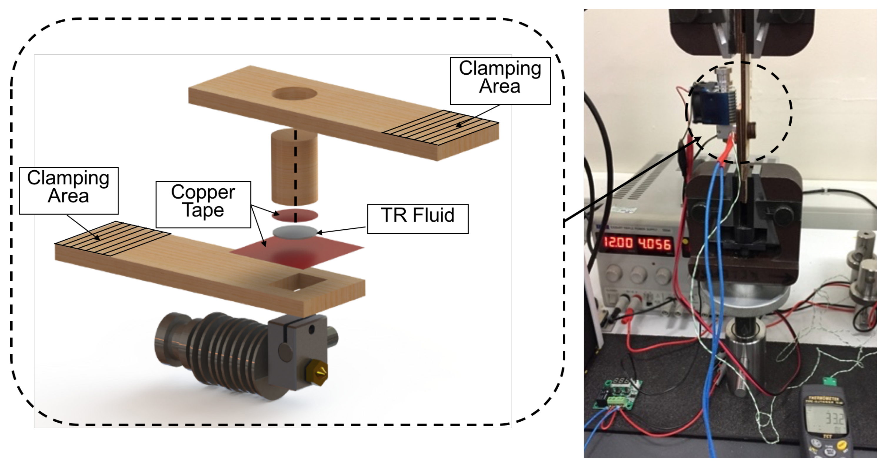
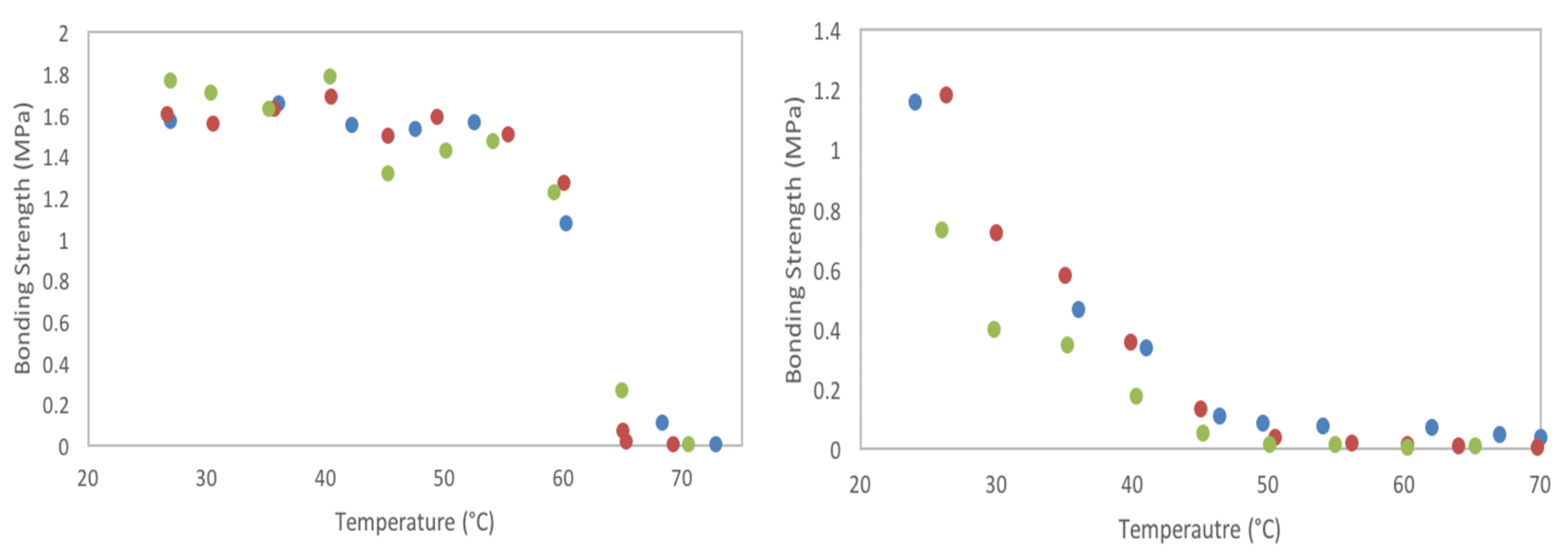
2.1. Temperature Effect on Bonding Strength
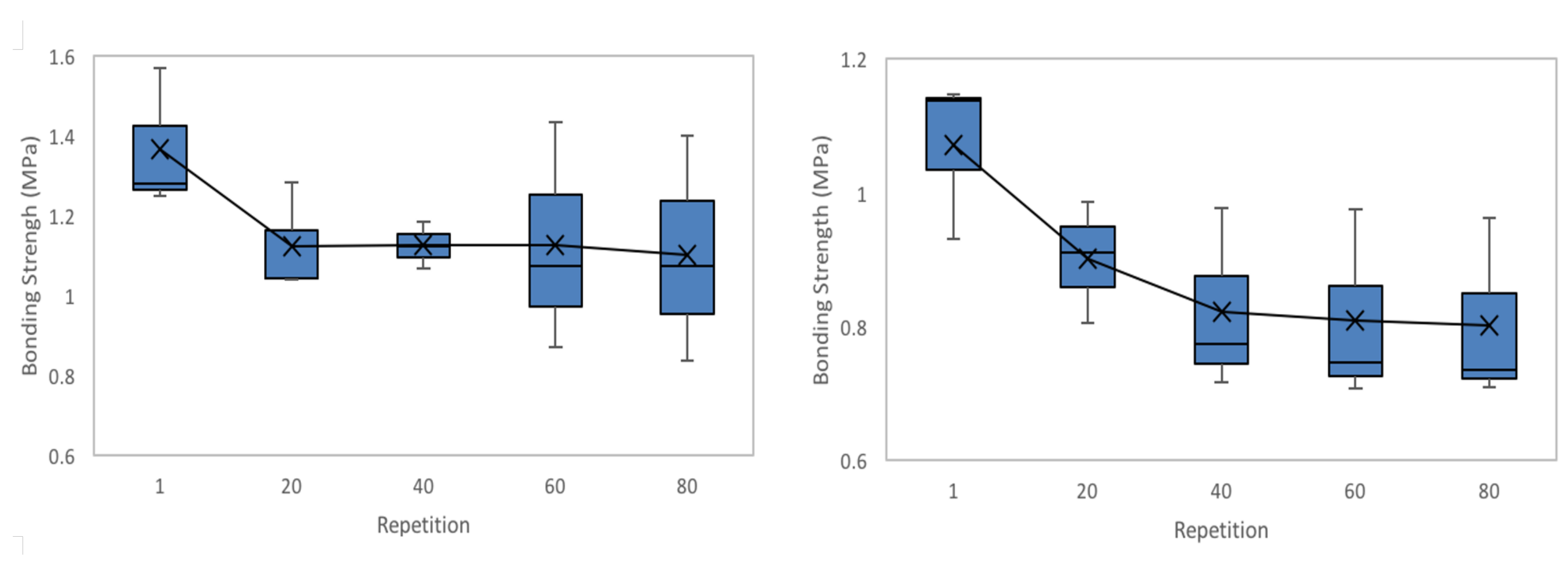
2.2. Repeatability
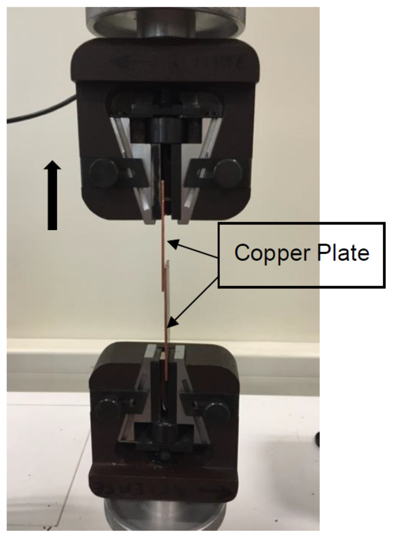
2.3. Adherend-Dependent Bonding Strength
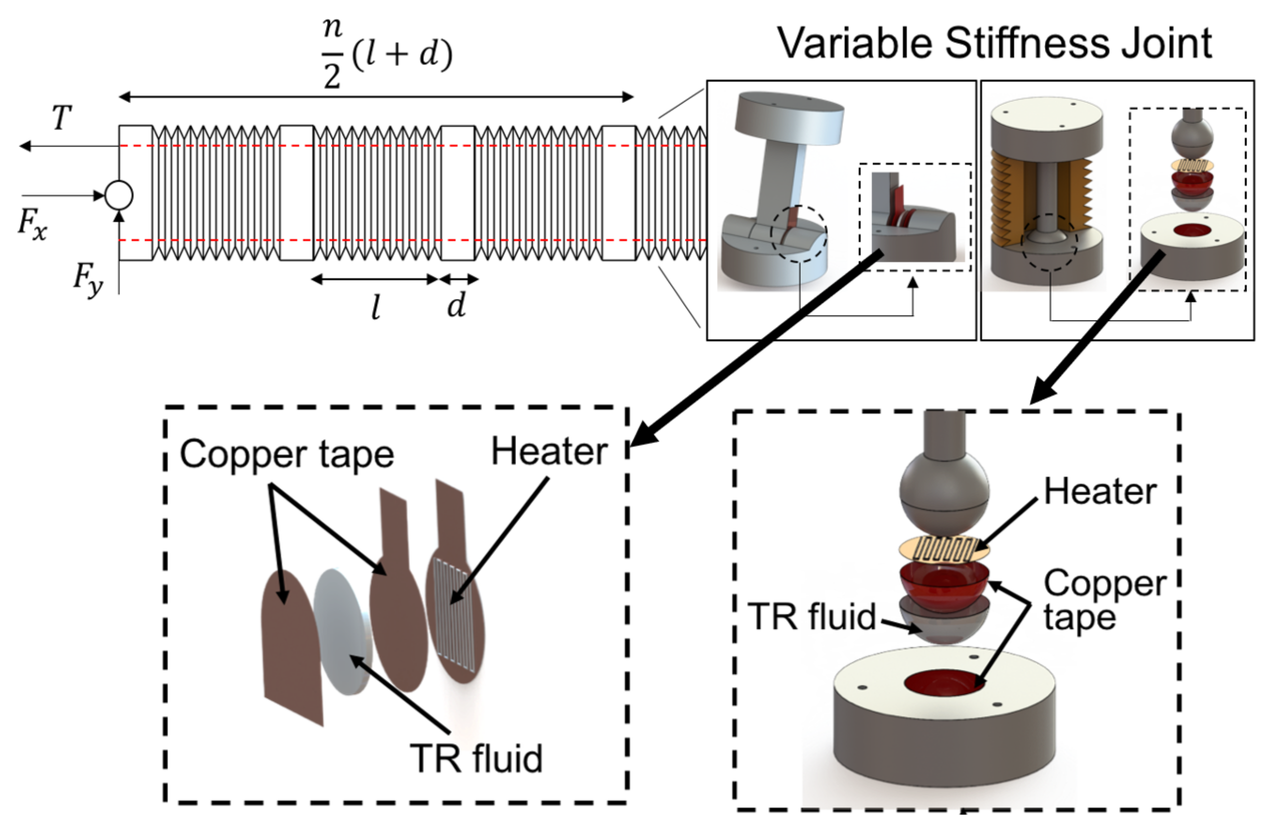
3. Controllable Variable Stiffness Joint Design and Simulation
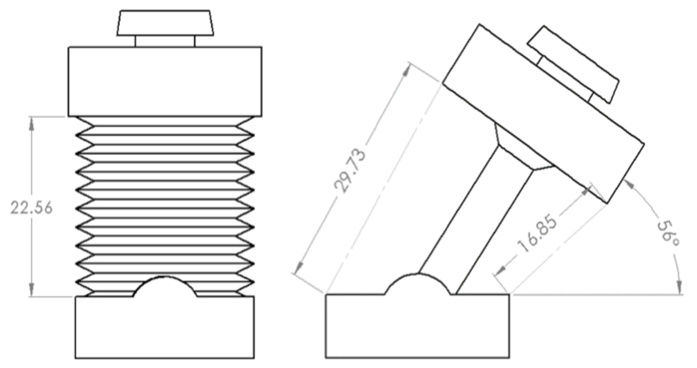
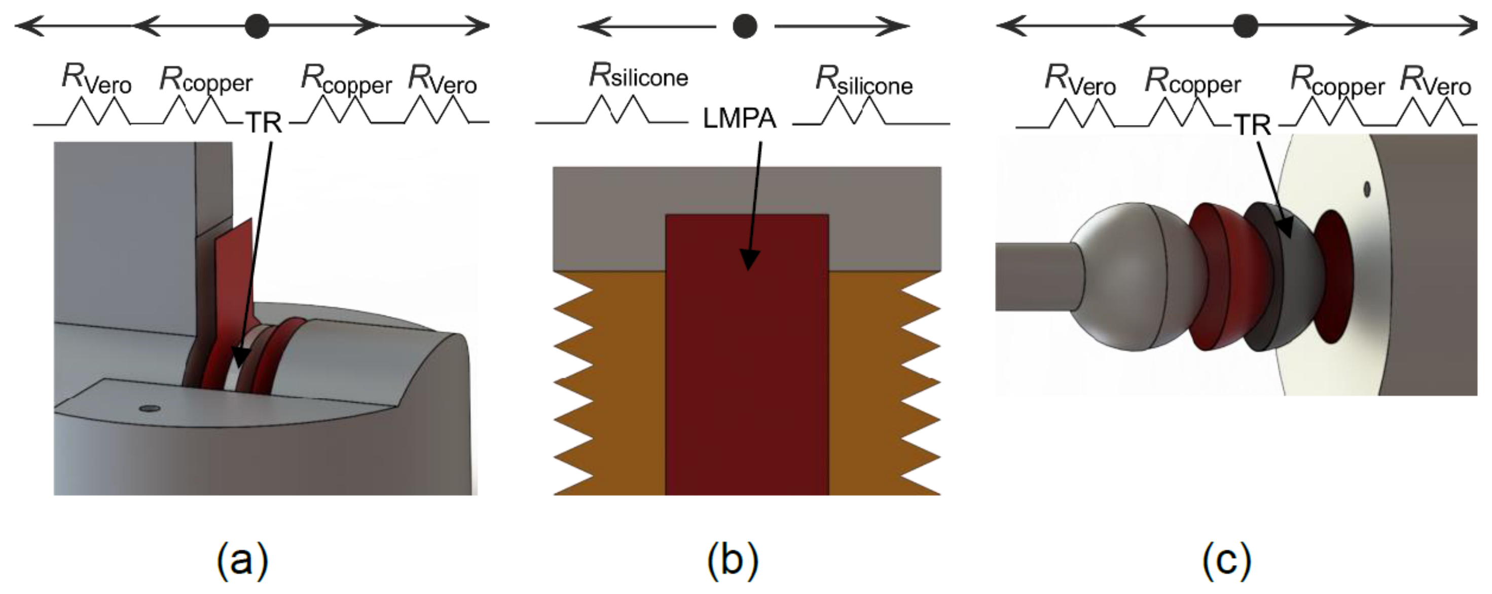
3.1. Design of Controllable Stiffness Joints
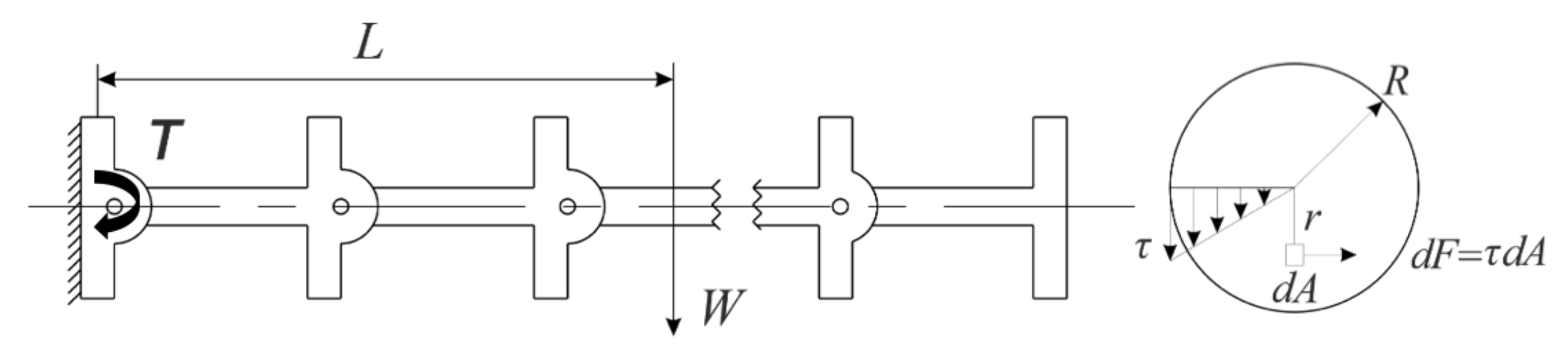
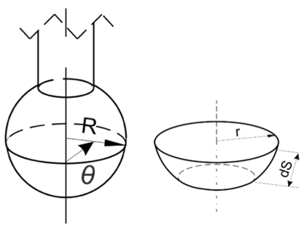
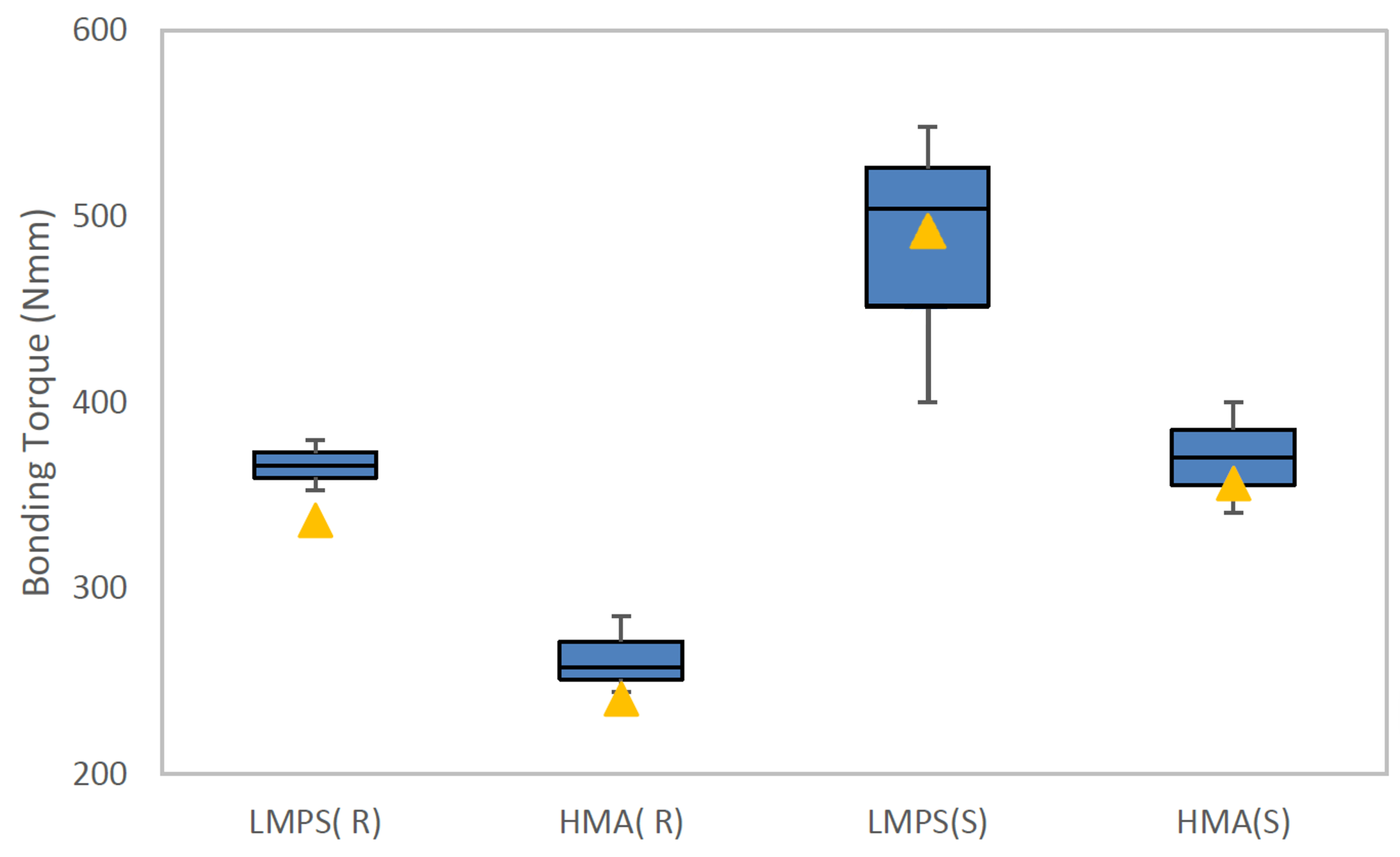
3.2. Bonding Torque Analysis
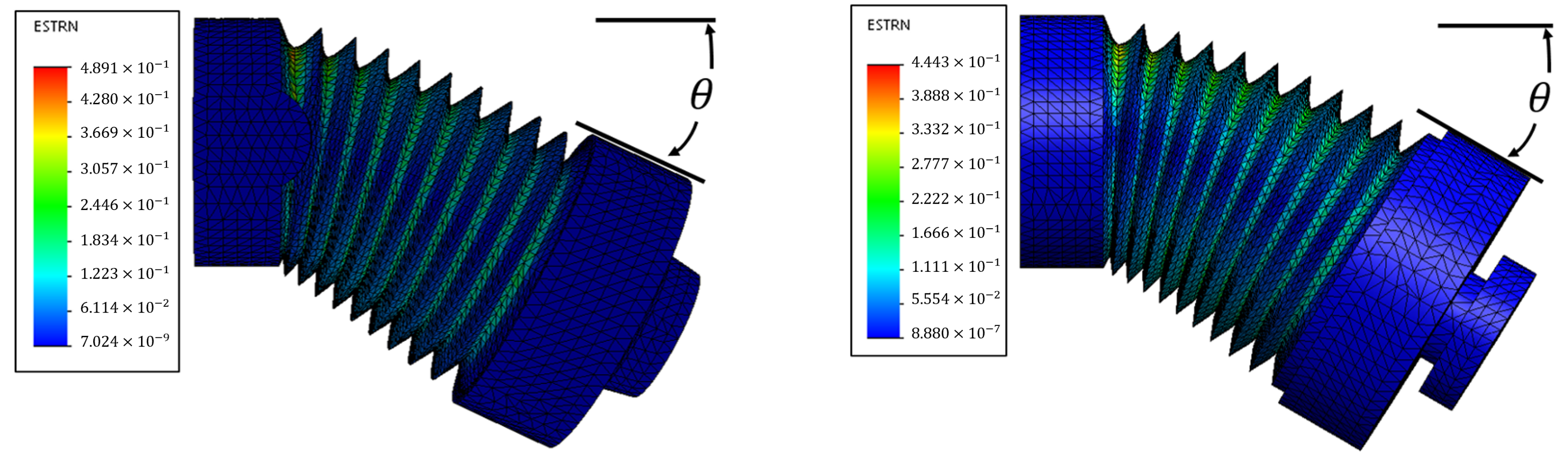
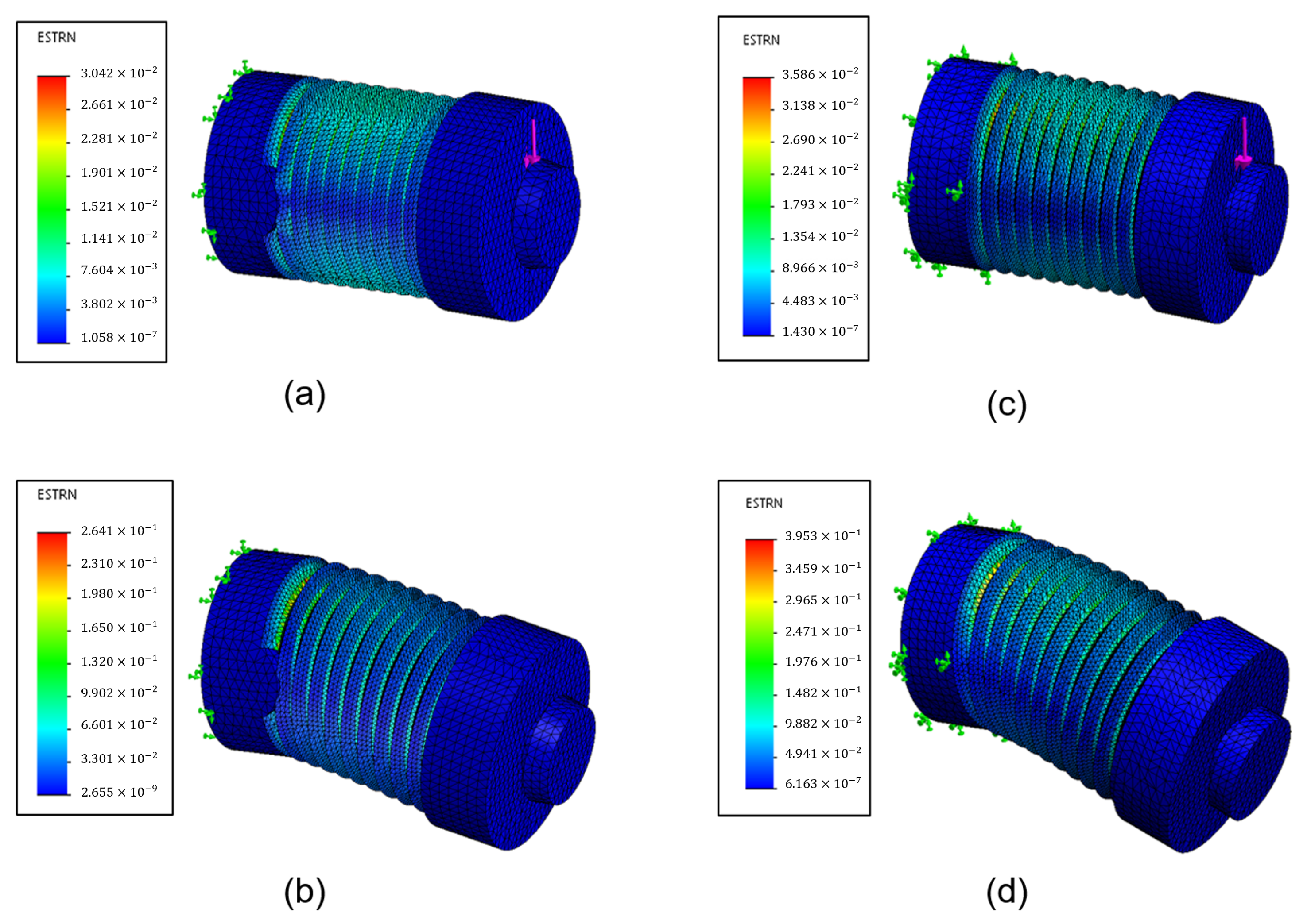
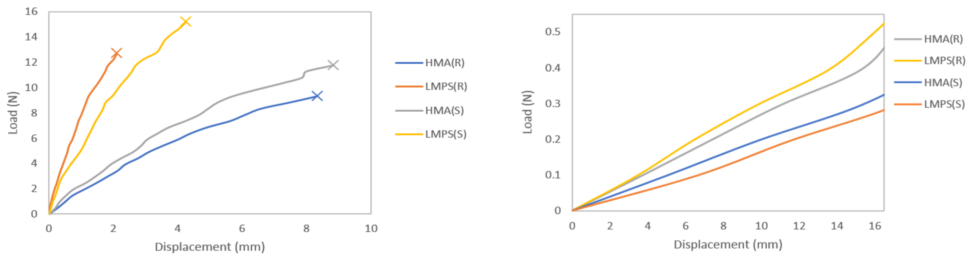
3.3. Joint Stiffness Simulation in Rigid and Soft States
3.4. Joint Heating and Cooling Processes
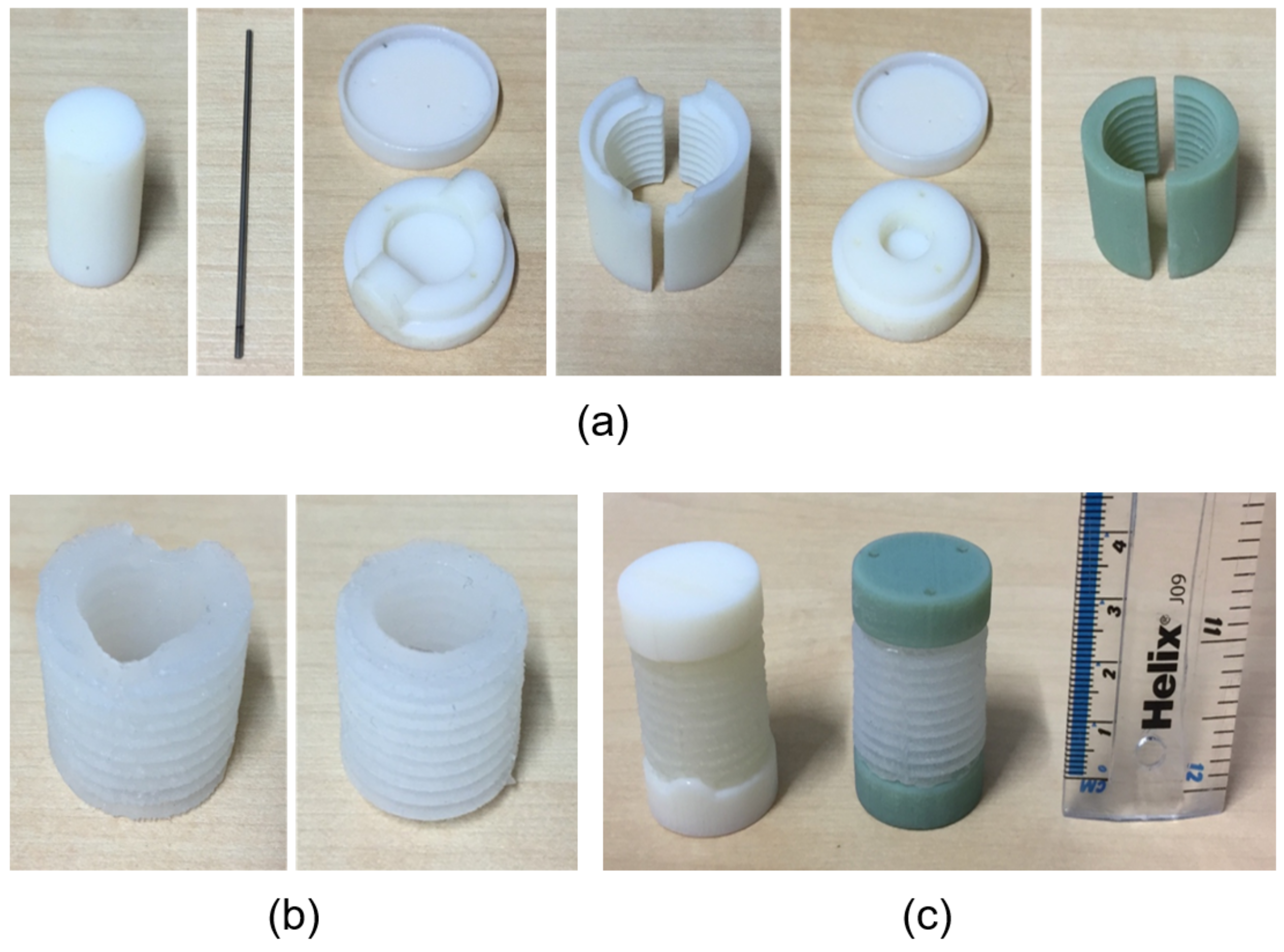
4. Robotic Joint Fabrication
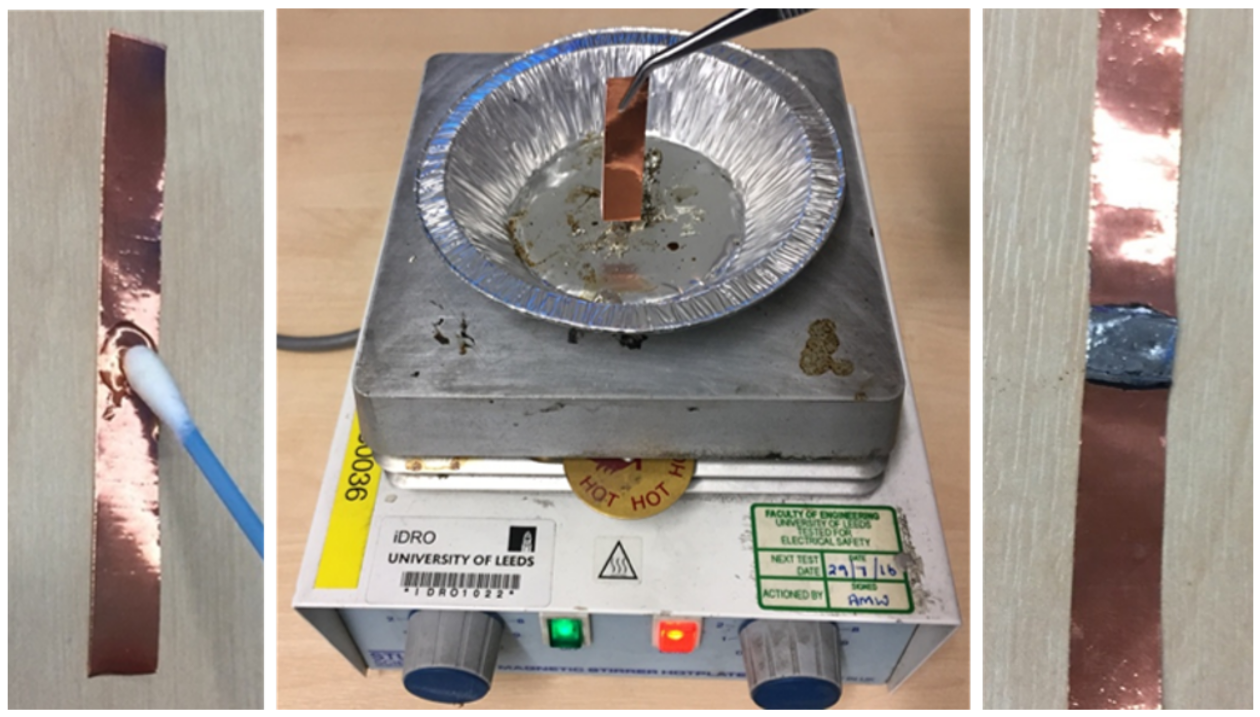
4.1. TR Fluids Application
4.2. Joint Fabrication
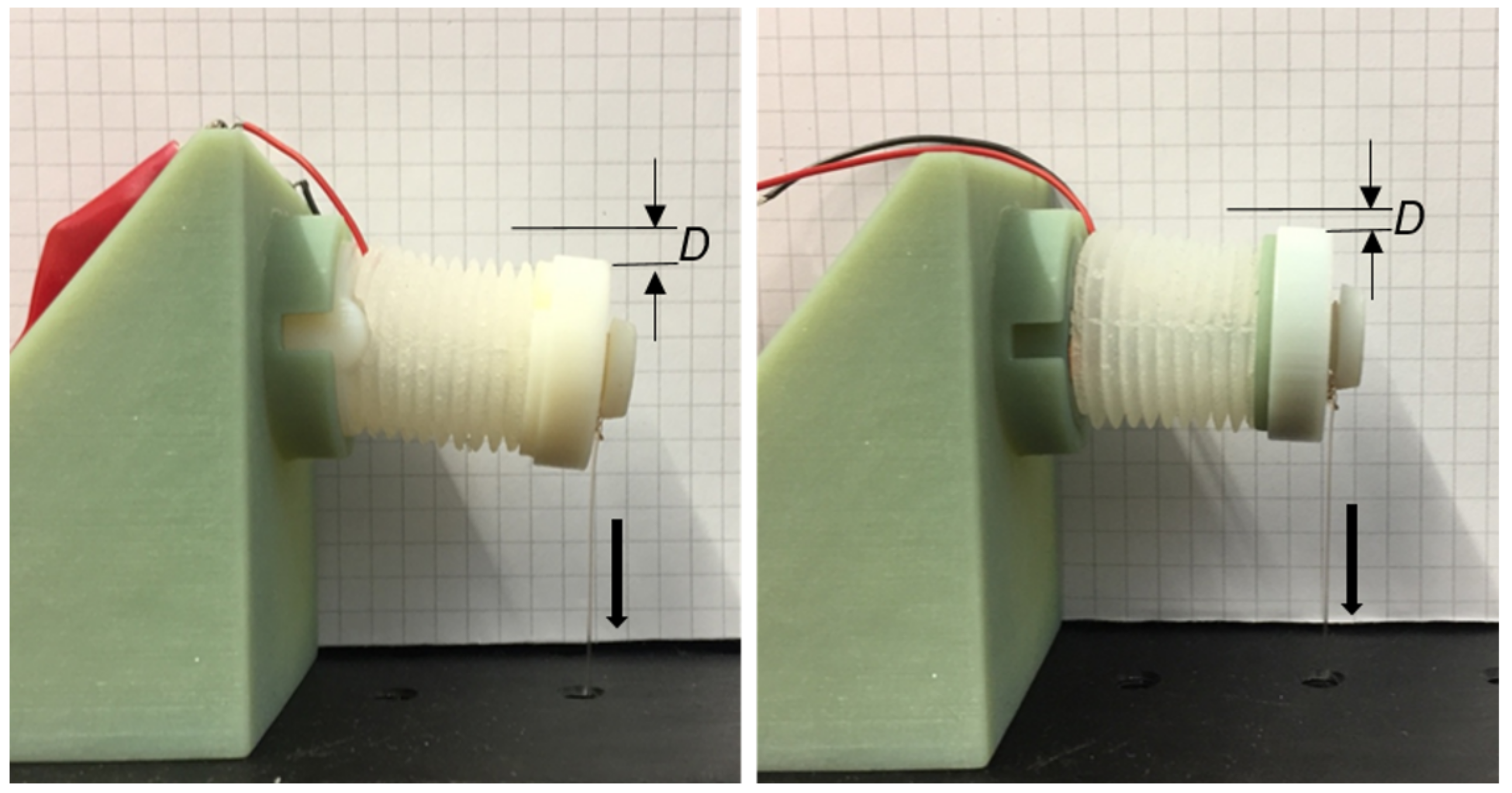
5. Experimental Validation
6. Conclusions
Author Contributions
Funding
Institutional Review Board Statement
Informed Consent Statement
Data Availability Statement
Conflicts of Interest
References
- Ding, J.; Goldman, R.E.; Xu, K.; Allen, P.K.; Fowler, D.L.; Simaan, N. Design and coordination kinematics of an insertable robotic effectors platform for Single-Port access surgery. IEEE/ASME Trans. Mechatron. 2013, 18, 1612–1624. [Google Scholar] [CrossRef] [PubMed] [Green Version]
- Shang, J.; Payne, C.J.; Clark, J.; Noonan, D.P.; Kwok, K.W.; Darzi, A.; Yang, G.Z. Design of a multitasking robotic platform with flexible arms and articulated head for minimally invasive surgery. In Proceedings of the IEEE/RSJ International Conference on Intelligent Robots and Systems, Vilamoura-Algarve, Portugal, 7–12 October 2012; pp. 1988–1993. [Google Scholar]
- Kwok, K.W.; Tsoi, K.H.; Vitiello, V.; Clark, J.; Chow, G.; Luk, W.; Yang, G.Z. Dimensionality reduction in controlling articulated snake robot for endoscopy under dynamic active constraints. IEEE Trans. Robot. 2013, 29, 15–31. [Google Scholar] [CrossRef] [PubMed] [Green Version]
- Wright, C.; Buchan, A.; Brown, B.; Geist, J.; Schwerin, M.; Rollinson, D.; Tesch, M.; Choset, H. Design and architecture of the unified modular snake robot. In Proceedings of the IEEE International Conference on Robotics and Automation, Saint Paul, MN, USA, 14–18 May 2012; pp. 4347–4354. [Google Scholar]
- Wright, C.; Johnson, A.; Peck, A.; McCord, Z.; Naaktgeboren, A.; Gianfortoni, P.; Gonzales-Rivero, M.; Hatton, R.; Choset, H. Design of modular snake robot. In Proceedings of the IEEE International Conference on Intelligent Robots and Systems, San Diego, CA, USA, 29 October–2 November 2007; pp. 2609–2614. [Google Scholar]
- Mehling, J.S.; Diftler, M.A.; Chu, M.; Valvo, M. A minimally invasive tendril robot for in-space inspection. In Proceedings of the IEEE/RAS-EMBS International Conference on Biomedical Robotics and Biomechatronics, Pisa, Italy, 20–22 February 2006; pp. 690–695. [Google Scholar]
- Gravagne, I.A.; Walker, I.D. Large deflection dynamics and control for planar continuum robots. IEEE/ASME Trans. Mechatron. 2003, 8, 299–307. [Google Scholar] [CrossRef] [Green Version]
- Mahvash, M.; Zenat, M. Toward a hybrid snake robot for single-port surgery. In Proceedings of the Annual International Conference of the IEEE Engineering in Medicine and Biology Society, Boston, MA, USA, 30 August–3 September 2011; pp. 5372–5375. [Google Scholar]
- Trivedi, D.; Rahn, C.D.; Kier, W.M.; Walker, I.D. Soft robotics: Biological inspiration, state of the art, and future research. Appl. Bionics Biomech. 2008, 5, 99–117. [Google Scholar] [CrossRef]
- Kim, S.; Laschi, C.; Trimmer, B. Soft robotics: A bioinspired evolution in robotics. Trends Biotechnol. 2013, 31, 287–294. [Google Scholar] [CrossRef]
- Simaan, N.; Taylor, R.; Flint, P. High Dexterity Snake-like Robotic Slaves for Minimally Invasive Telesurgery of the Upper Airway. In Proceedings of the International Conference on Medical Image Computing and Computer- Assisted Intervention, St. Malo, France, 26–29 September 2004; pp. 17–24. [Google Scholar]
- Simaan, N.; Taylor, R.; Flint, P. A dexterous system for laryngeal surgery. In Proceedings of the IEEE International Conference on Robotics and Automation, New Orleans, LA, USA, 26 April–1 May 2004; pp. 351–357. [Google Scholar]
- Degani, A.; Choset, H.; Wolf, A.; Zenat, M.A. Highly Articulated Robotic Probe for Minimally Invasive Surgery. In Proceedings of the IEEE International Conference on Robotics and Automation, Orlando, FL, USA, 15–19 May 2006; pp. 4167–4172. [Google Scholar]
- Degani, A.; Choset, H.; Wolf, A.; Ota, T.; Zenati, M.A. Percutaneous Intrapericardial Interventions Using a Highly Articulated Robotic Probe. In Proceedings of the IEEE / RAS-EMBS International Conference on Biomedical Robotics and Biomechatronics, Pisa, Italy, 20–22 February 2006; pp. 7–12. [Google Scholar]
- Chen, Y.; Chang, J.H.; Greenlee, A.S.; Cheung, K.C.; Slocum, A.H.; Gupta, R. Multi-turn, tension-stiffening catheter navigation system. In Proceedings of the IEEE International Conference on Robotics and Automation, Anchorage, AK, USA, 3–7 May 2010; pp. 5570–5575. [Google Scholar]
- Manti, M.; Cacucciolo, V.; Cianchetti, M. Stiffening in soft robotics: A review of the state of the art. IEEE Robot. Autom. 2016, 23, 93–106. [Google Scholar] [CrossRef]
- Majidi, C.; Wood, R.J. Tunable elastic stiffness with micro-confined magnetorheological domains at low magnetic field. Appl. Phys. Lett. 2010, 97, 164104. [Google Scholar] [CrossRef]
- Liu, B.; Boggs, S.A.; Shaw, M.T. Electrorheological Properties of Anisotropically Filled Elastomers. IEEE Trans. DEI 2001, 8, 173–181. [Google Scholar] [CrossRef]
- Cao, C.; Zhao, X. Tunable stiffness of electrorheological elasto-mers by designing mesostructures. Appl. Phys. Lett. 2013, 103, 041901. [Google Scholar] [CrossRef] [Green Version]
- Cheng, N.; Ishigami, G.; Hawthorne, S.; Hao, C.; Hansen, M.; Telleria, M.; Playter, R.; Iagnemma, K. Design and analysis of a soft mobile robot composed of multiple thermally activated joints driven by a single actuator. In Proceedings of the IEEE International Conference on Robotics and Automation, Anchorage, AK, USA, 3–7 May 2010; pp. 5207–5212. [Google Scholar]
- Telleria, M.; Hansen, M.; Campbell, D.; Servi, A.; Culpepper, M. Modeling and implementation of solder-activated joints for single-actuator, centimeter-scale robotic mechanisms. In Proceedings of the IEEE International Conference on Robotics and Automation, Anchorage, AK, USA, 3–7 May 2010; pp. 1681–1686. [Google Scholar]
- Neubert, J.; Rost, A.; Lipson, H. Self-soldering connectors for modular robots. IEEE Trans. Robot. 2014, 30, 1344–1357. [Google Scholar] [CrossRef]
- Cheng, N.G.; Gopinath, A.; Wang, L.; Iagnemma, K.; Hosoi, A.E. Thermally tunable, self-healing composites for soft robotic applications. Macromol. Mater. Eng. 2014, 299, 1279–1284. [Google Scholar] [CrossRef]
- Cheng, N.G.; Lobovsky, M.B.; Keating, S.J.; Setapen, A.M.; Gero, K.I.; Hosoi, A.E.; Iagnemma, K.D. Design and analysis of a robust, low-cost, highly articulated manipulator enabled by jamming of granular media. In Proceedings of the IEEE International Conference on Robotics and Automation, St. Paul, MN, USA, 14–18 May 2012; pp. 4328–4333. [Google Scholar]
- Cianchetti, M.; Ranzani, T.; Gerboni, G.; Falco, I.D.; Laschi, C.; Menciassi, A. STIFF-FLOP Surgical Manipulator: Mechanical design and experimental characterization of the single module. In Proceedings of the IEEE/RSJ nternational Conference on Intelligent Robots and Systems, Tokyo, Japan, 3–7 November 2013; pp. 3576–3581. [Google Scholar]
- Ranzani, T.; Cianchetti, M.; Gerboni, G.; Falco, I.D.; Menciassi, A. A Soft Modular Manipulator for Minimally Invasive Surgery: Design and Characterization of a Single Module. IEEE Trans. Robot. 2016, 32, 187–200. [Google Scholar] [CrossRef]
- Kim, Y.J.; Cheng, S.; Kim, S.; Iagnemma, K. Design of a tubular snake-like manipulator with stiffening capability by layer jamming. In Proceedings of the International Conference on Intelligent Robots and Systems, Vilamoura-Algarve, Portugal, 7–12 October 2012; pp. 4251–4256. [Google Scholar]
- Kim, Y.J.; Cheng, S.; Kim, S.; Iagnemma, K. A novel layer jamming mechanism with tunable stiffness capability for minimally invasive surgery. IEEE Trans. Robot. 2013, 29, 1031–1042. [Google Scholar] [CrossRef]
- Wang, L.; Iida, F. Physical connection and disconnection control based on hot melt adhesives. IEEE/ASME Trans. Mechatron. 2013, 18, 1397–1409. [Google Scholar] [CrossRef]
- Wang, L.; Graber, L.; Iida, F. Large-payload climbing in complex vertical environments using thermoplastic adhesive bonds. IEEE Trans. Robot. 2013, 29, 863–874. [Google Scholar] [CrossRef]
- Shintake, J.; Schubert, B.; Rosset, S.; Shea, H.; Floreano, D. Variable stiffness actuator for soft robotics using dielectric elastomer and low- melting-point alloy. In Proceedings of the IEEE/RSJ International Conference on Intelligent Robots and Systems, Hamburg, Germany, 28 September–2 October 2015; pp. 1097–1102. [Google Scholar]
- Schubert, B.E.; Floreano, D. Variable stiffness material based on rigid low-melting-point-alloy microstructures embedded in soft polydimethylsiloxane (PDMS). RSC Adv. 2013, 3, 24671–24679. [Google Scholar] [CrossRef] [Green Version]
- Lin, Y.; Yang, G.; Liang, Y.; Zhang, C.; Wang, W.; Qian, D.; Yang, H.; Zou, J. Controllable stiffness origami “skeletons” for lightweight and multifunctional artificial muscles. Adv. Funct. Mater. 2020, 30, 2000349. [Google Scholar] [CrossRef]
- Yang, Y.; Chen, Y. Novel design and 3D printing of variable stiffness robotic fingers based on shape memory polymer. In Proceedings of the 2016 6th IEEE International Conference on Biomedical Robotics and Biomechatronics (BioRob), Singapore, 26–29 June 2016. [Google Scholar]
- Li, X.; Zhu, H.; Lin, W.; Chen, W.; Low, K. Structure-Controlled Variable Stiffness Robotic Joint Based on Multiple Rotary Flexure Hinges. IEEE Trans. Ind. Electron. 2020, 68, 12452–12461. [Google Scholar] [CrossRef]
- SMOOTH-ON. Technical and Buying Information. Available online: https://www.smooth-on.com/product-line/dragon-skin/ (accessed on 28 April 2022).
- Huat, L.J. Customizable Soft Pneumatic Gripper Devices. Master’s Thesis, National University of Singapore, Singapore, 2015. [Google Scholar]
- Sparks, J.L.; Vavalle, N.A.; Kasting, K.E.; Long, B.; Tanaka, M.L.; Sanger, P.A.; Schnell, K.; Conner-Kerr, T.A. Use of silicone materials to simulate tissue biomechanics as related to deep tissue injury. Adv. Skin Wound Care 2015, 28, 59–68. [Google Scholar] [CrossRef]
- Martins, P.A.L.S.; Jorge, R.M.N.; Ferreora, A.J.M. A comparative study of several material models for prediction of hyperelastic properties: 73 application to silicone-rubber and soft tissues. Strain 2006, 42, 135–147. [Google Scholar] [CrossRef]
- Meghezi, S.; Couet, F.; Chevallier, P.; Mantovani, D. Effects of a pseudophysiological environment on the elastic and viscoelastic properties of collagen gels. Int. J. Biomater. 2012, 2012, 319290. [Google Scholar] [CrossRef] [PubMed] [Green Version]
- Ali, A.; Hosseini, M.; Sahari, B.B. A review of constitutive models for rubber-like materials. Am. J. Eng. Appl. Sci. 2010, 3, 232–239. [Google Scholar] [CrossRef] [Green Version]
- Case, J.; White, E.; Kramer, R. Soft material characterization for robotic applications. Soft Robot. 2015, 2, 80–87. [Google Scholar] [CrossRef]
- Marechal, L.; Balland, P.; Lindenroth, L.; Petrou, F.; Kontovounisios, C.; Bello, F. Toward a common framework and database of materials for soft robotics. Soft Robot. 2021, 8, 284–297. [Google Scholar] [CrossRef] [PubMed]
- ASTM Standard D412, 06a; Standard Test Methods for Vulcanized Rubber and Thermoplastic Elastomers-Tension. ASTM International: West Conshohocken, PA, USA, 2013.


| Material | Shear Strength (MPa) |
|---|---|
| Aluminium | 1.0562 ± 0.1770 |
| Copper | 1.0496 ± 0.2443 |
| Plastic | 0.1846 ± 0.0373 |
| Joint Type | LMPS Bonding Torque | HMA Bonding Torque |
|---|---|---|
| Revolute Joint | 336.75 Nmm | 240.46 Nmm |
| Spherical Joint | 495.79 Nmm | 356.47 Nmm |
| State | Load | Displacement | Max Strain | Stiffness Constant |
|---|---|---|---|---|
| Bonding (R) | 5.88 N | 1.101 mm | 0.03042 | 5.3406 N/mm |
| Soft (R) | 0.196 N | 7.291 mm | 0.2641 | 0.0269 N/mm |
| Bonding (S) | 5.88 N | 1.174 mm | 0.03586 | 5.0085 N/mm |
| Soft (S) | 0.196 N | 11.488 mm | 0.3953 | 0.0171 N/mm |
| Joint Type | LMPS Bonding Torque | HMA Bonding Torque |
|---|---|---|
| Revolute Joint | 379.91 Nmm | 262.32 Nmm |
| Spherical Joint | 484.20 Nmm | 370.56 Nmm |
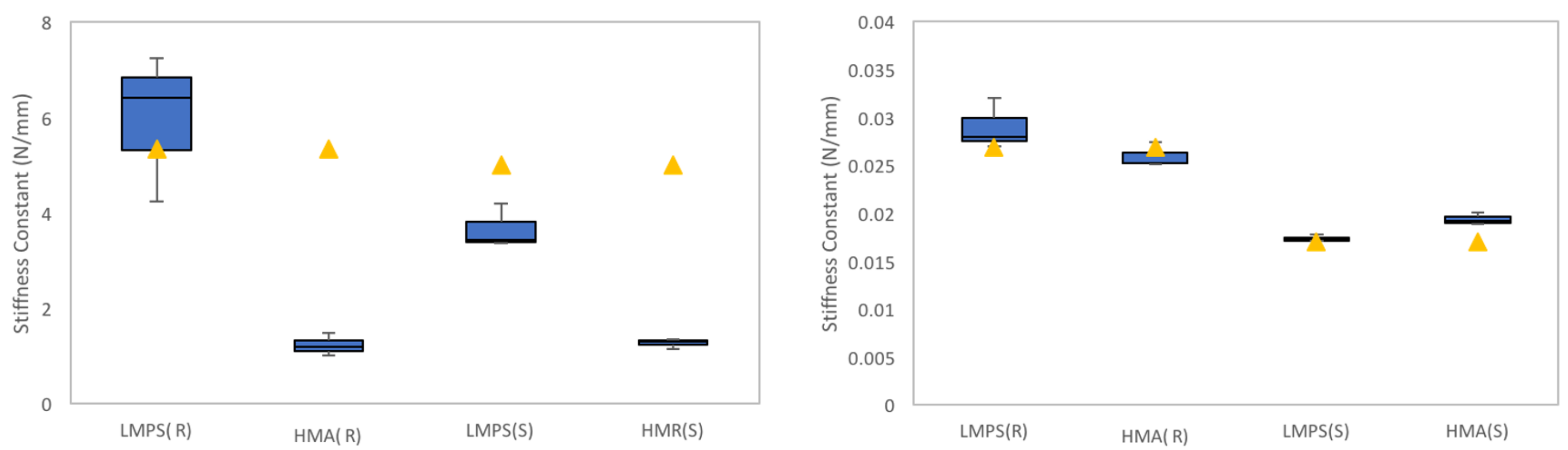
| Joint Material | Stiffness Constant in Soft State (N/mm) | Stiffness Constant in Bonding State (N/mm) | Stiffness Increase Ratio |
|---|---|---|---|
| LMPS (R) | 0.029 ± 0.0026 | 5.969 ± 1.5594 | 205.8 |
| HMA (R) | 0.026 ± 0.0013 | 1.228 ± 0.2332 | 47.2 |
| LMPS (S) | 0.017 ± 0.0004 | 3.669 ± 0.4678 | 215.8 |
| HMA (S) | 0.021 ± 0.0006 | 1.274 ± 0.1131 | 60.7 |
| LMPS(R) | HMA(R) | LMPS(S) | HMA(S) | |
|---|---|---|---|---|
| Power (W) | 2.9 ± 0.2 | 3.7 ± 0.4 | 3.6 ± 0.1 | 2.7 ± 0.5 |
| Activation Time (s) | 13.0 ± 3.9 | 8.0 ± 1.5 | 29.4 ± 7.8 | 18.6 ± 2.5 |
| Deactivation Time (s) | 7.8 ± 1.9 | 42.7 ± 7.2 | 18.5 ± 2.8 | 30.2 ± 5.8 |
Publisher’s Note: MDPI stays neutral with regard to jurisdictional claims in published maps and institutional affiliations. |
© 2022 by the authors. Licensee MDPI, Basel, Switzerland. This article is an open access article distributed under the terms and conditions of the Creative Commons Attribution (CC BY) license (https://creativecommons.org/licenses/by/4.0/).
Share and Cite
Ma, B.; Shaqura, M.Z.; Richardson, R.C.; Dehghani-Sanij, A.A. A Study on Phase-Changing Materials for Controllable Stiffness in Robotic Joints. Robotics 2022, 11, 66. https://doi.org/10.3390/robotics11030066
Ma B, Shaqura MZ, Richardson RC, Dehghani-Sanij AA. A Study on Phase-Changing Materials for Controllable Stiffness in Robotic Joints. Robotics. 2022; 11(3):66. https://doi.org/10.3390/robotics11030066
Chicago/Turabian StyleMa, Bingyin, Mohammed Z. Shaqura, Robert C. Richardson, and Abbas A. Dehghani-Sanij. 2022. "A Study on Phase-Changing Materials for Controllable Stiffness in Robotic Joints" Robotics 11, no. 3: 66. https://doi.org/10.3390/robotics11030066
APA StyleMa, B., Shaqura, M. Z., Richardson, R. C., & Dehghani-Sanij, A. A. (2022). A Study on Phase-Changing Materials for Controllable Stiffness in Robotic Joints. Robotics, 11(3), 66. https://doi.org/10.3390/robotics11030066