
Multi-Fidelity Information Fusion to Model the Position-Dependent Modal Properties of Milling Robots


Abstract
:1. Introduction
1.1. Related Work
- conventional rigid-body models [9],
- rigid-body models with additional virtual joints [10] or
- finite element models [11].
1.2. Motivation
1.3. Scope and Approach
2. Methods
- the natural frequencies for each vibration mode of the robot structure,
- the damping ratios for each vibration mode of the robotstructure and
- the residues for each vibration mode and in each mode direction .
- Data generation: first, the modal parameters are derived from the analytical model and gathered experimentally at the robot (see Section 2.1).
- Data preparation: the data sets are divided into training and testing data sets (see Section 2.2).
- Model setup and training: the spatial behavior of the vibrational features is modeled as follows (see Section 2.3):
- (a)
- The primary features (natural frequencies) are modeled using multi-fidelity information fusion approaches (see Section 2.3.1).
- (b)
- The secondary features (damping ratios and residues) are modeled using conventional Gaussian process regression techniques (see Section 2.3.2 and Section 2.3.3).
2.1. Data Generation: Spatial Modal Parameter Identification
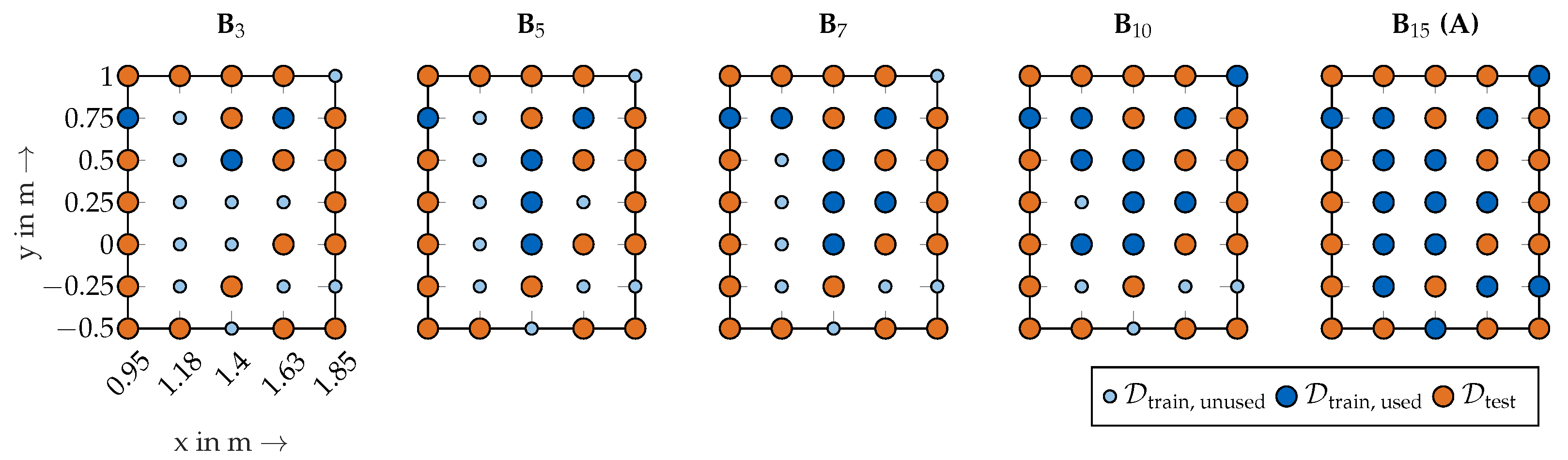
2.2. Data Preparation: Sampling Methodology
- The testing data set remains the same for all investigations.
- The actually used training data points are subsampled from the original training data set .
2.3. Model Setup and Training: Data Driven Modeling of the Modal Properties
- natural frequencies (Section 2.3.1),
- damping ratios (Section 2.3.2) and
- residues (Section 2.3.3).
2.3.1. Primary Feature: Natural Frequencies
- a linear kernel: a linear kernel makes it possible to incorporate a linear spatial model using the variance :
- a quadratic kernel: a quadratic kernel allows more flexibility than a simple linear kernel and is represented by
- a cubic kernel: similar to the generation of a quadratic kernel, the idea of a polynomial kernel can be extended to a cubic kernel, given by
- a radial basis function (RBF) kernel: the conventional RBF kernel is a very popular kernel, as no assumption on the data’s structure is incorporated. However, an RBF kernel may be prone to overfitting. The kernel is defined aswhere is the variance and l is the lengthscale of the RBF kernel.
2.3.2. Secondary Feature: Damping Ratios
2.3.3. Secondary Feature: Residues
3. Results
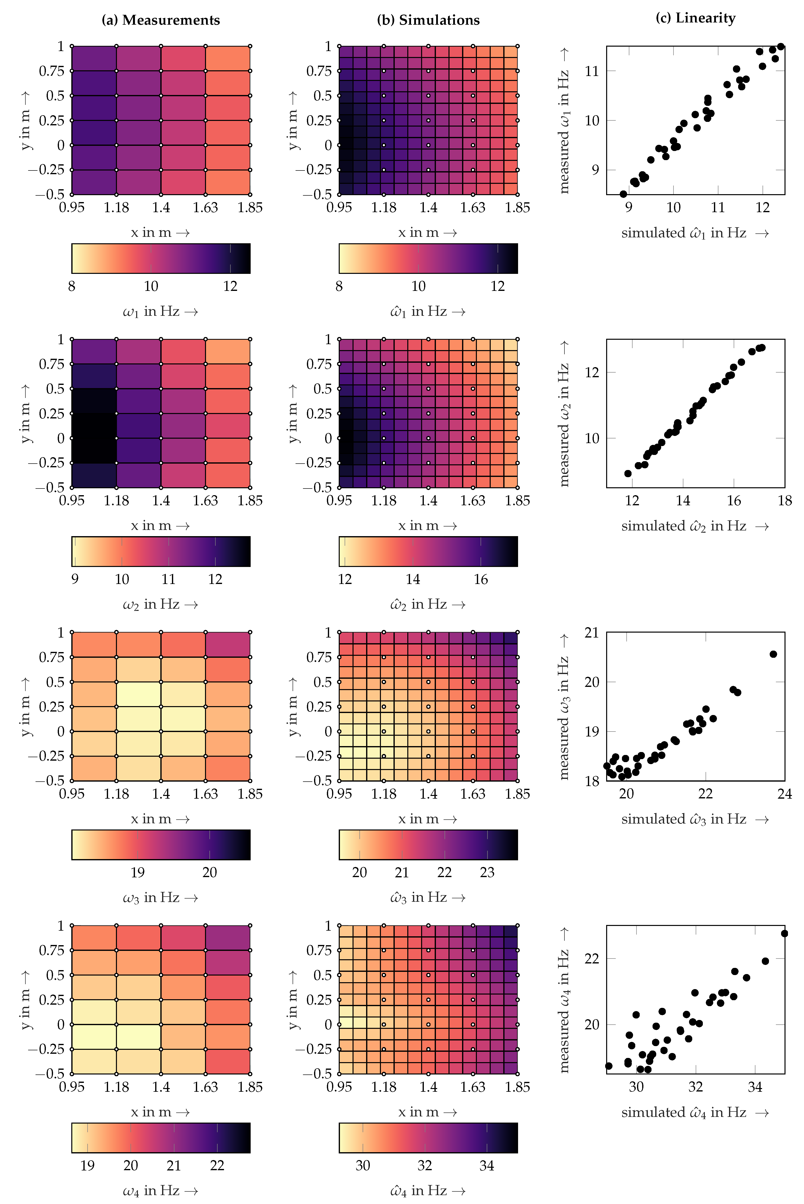
3.1. Primary Feature: Natural Frequencies
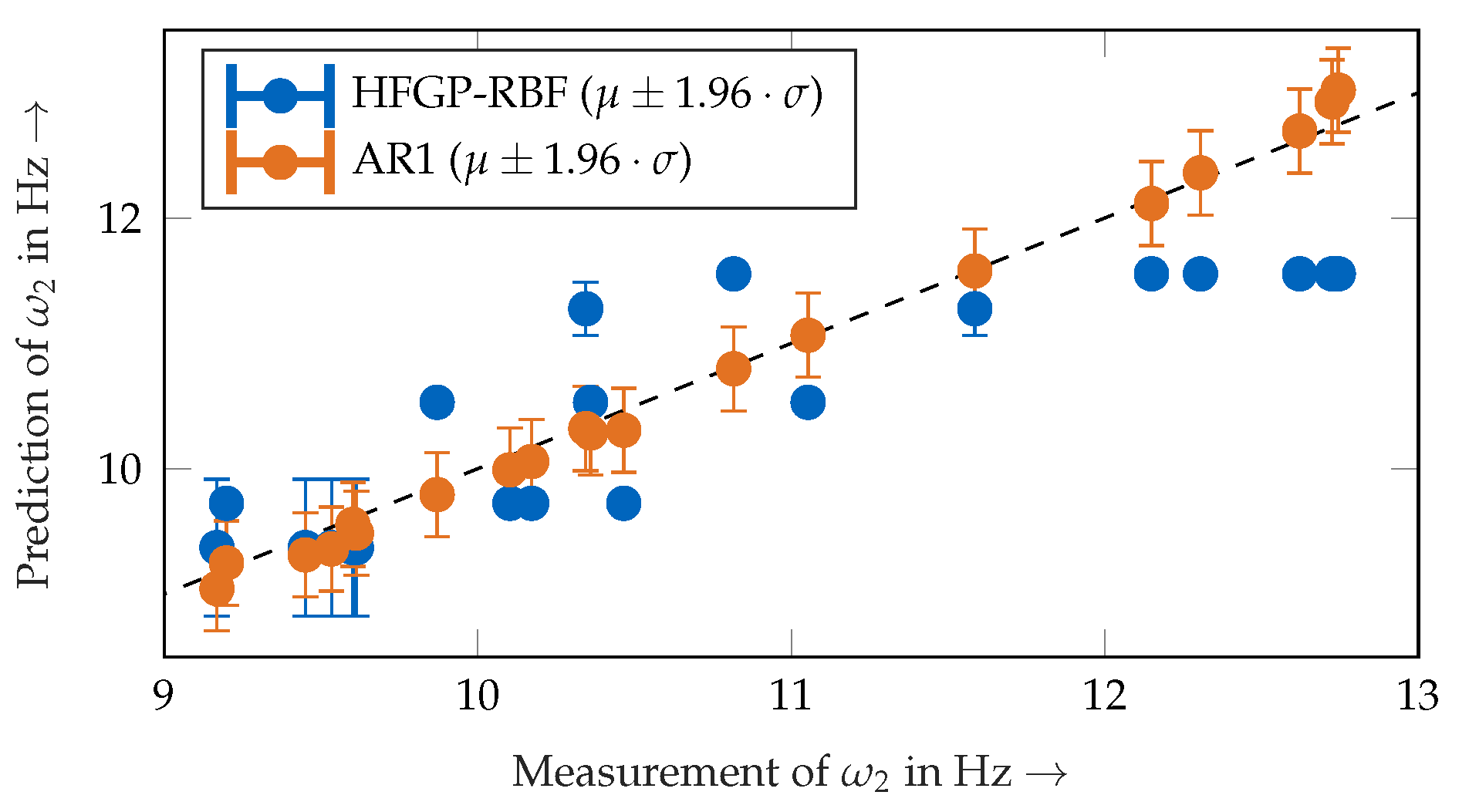
3.1.1. Validity of the Approach
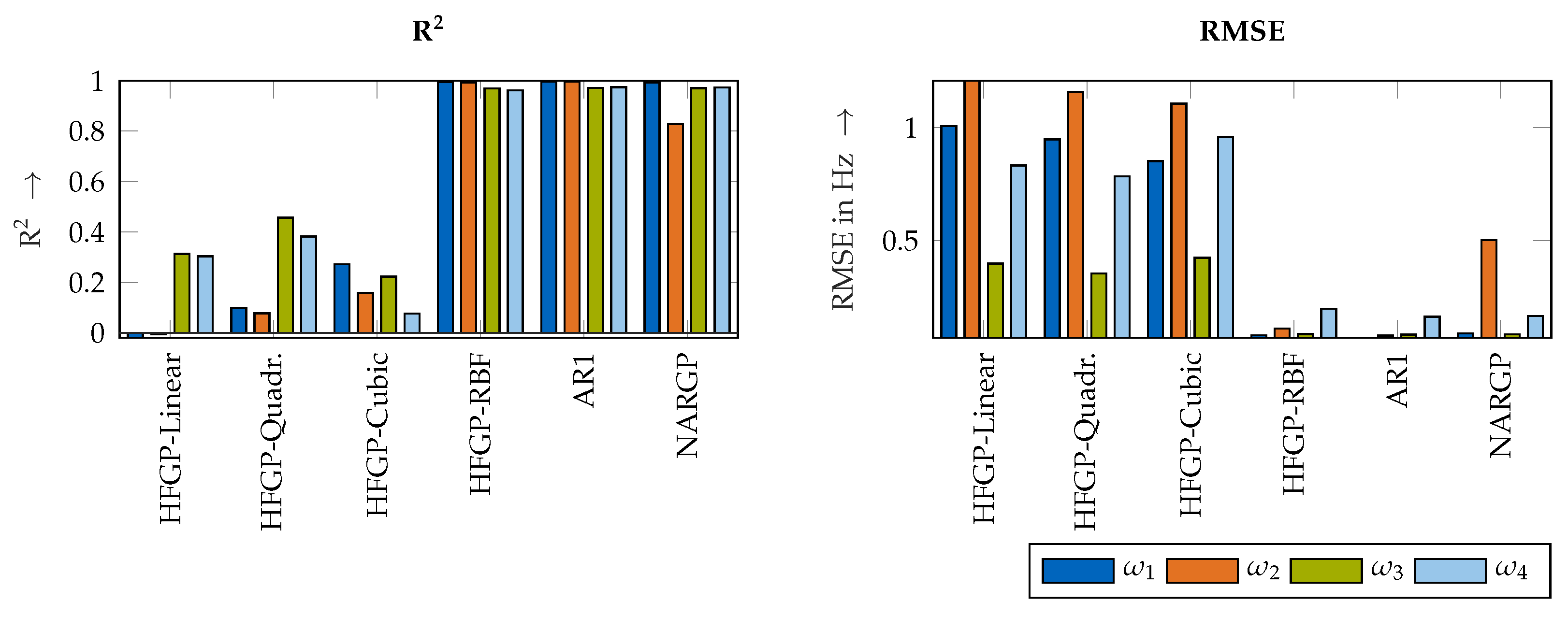
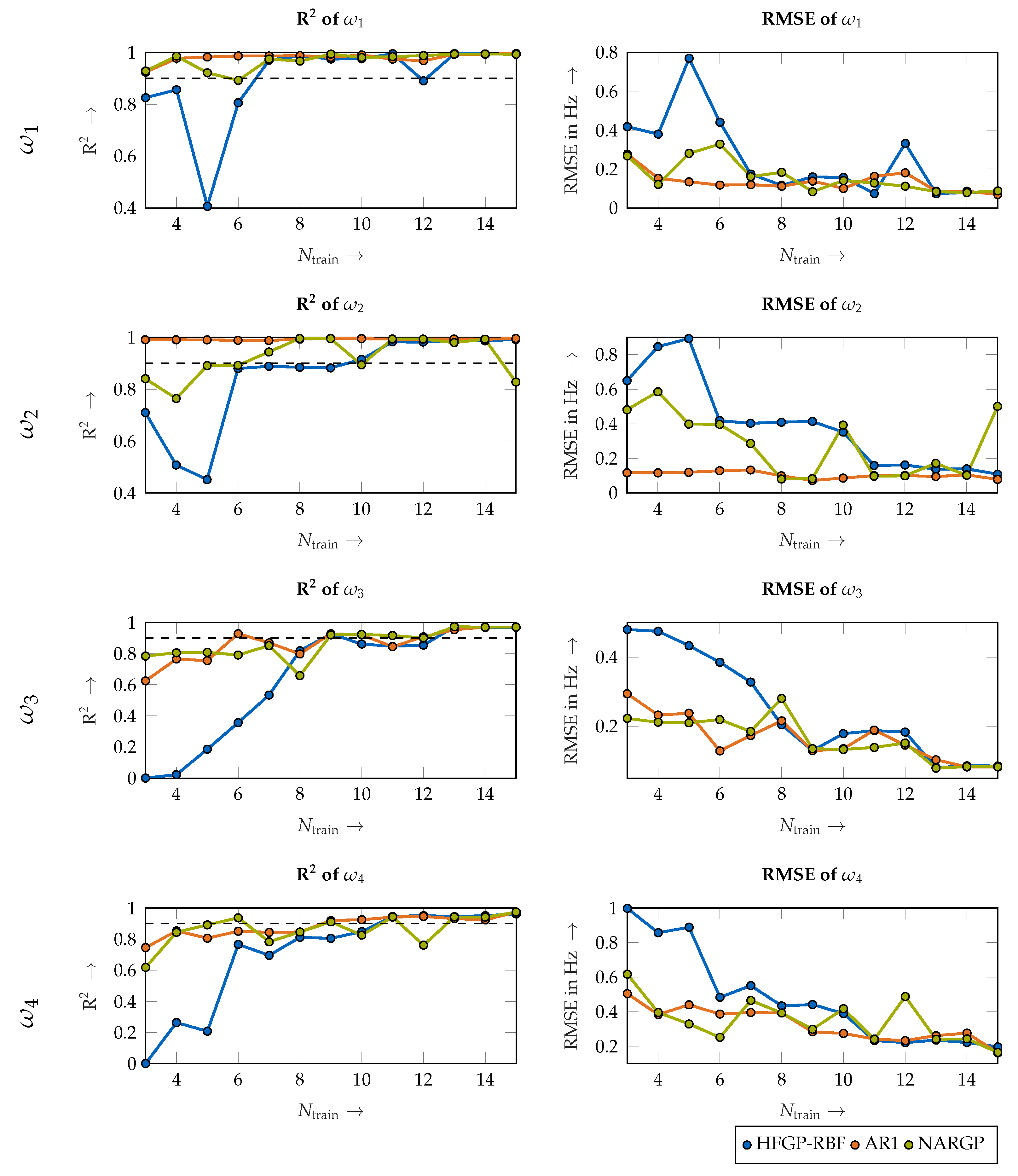
3.1.2. Accuracy Using an Increasing Number of Training Data Points
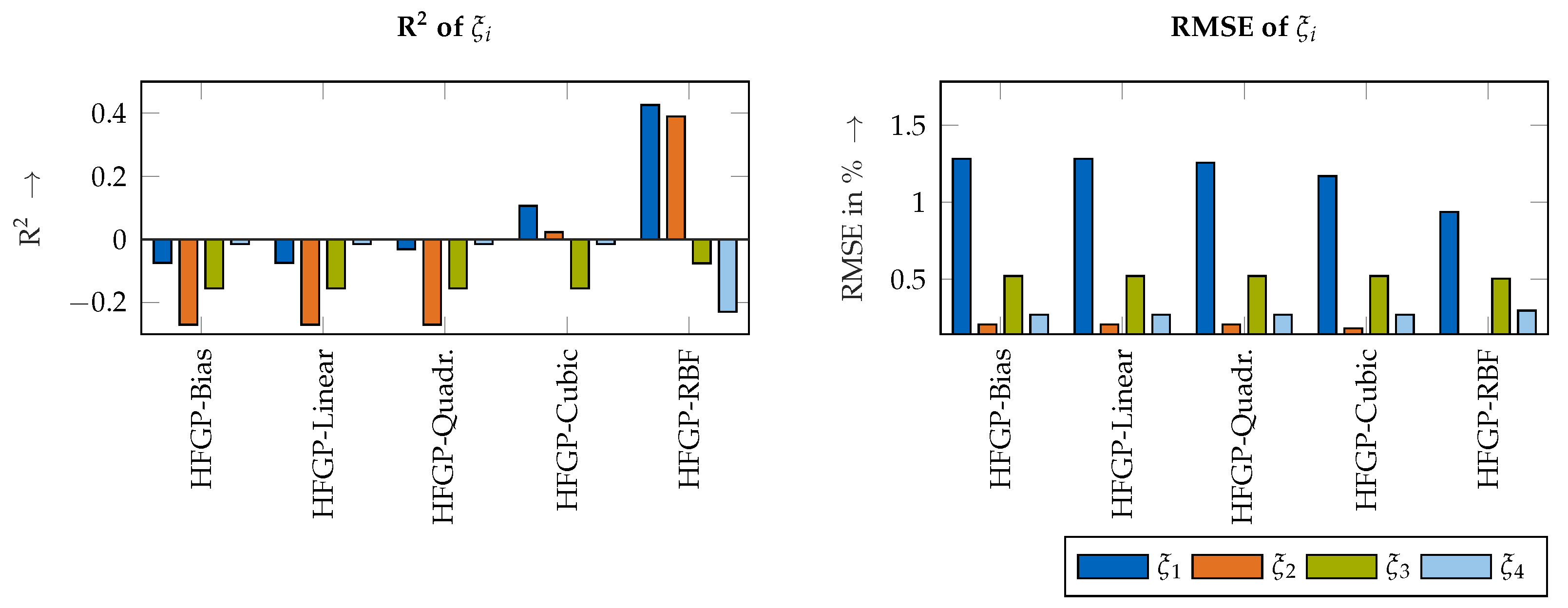
3.2. Secondary Feature: Damping Ratios
3.3. Secondary Feature: Residues
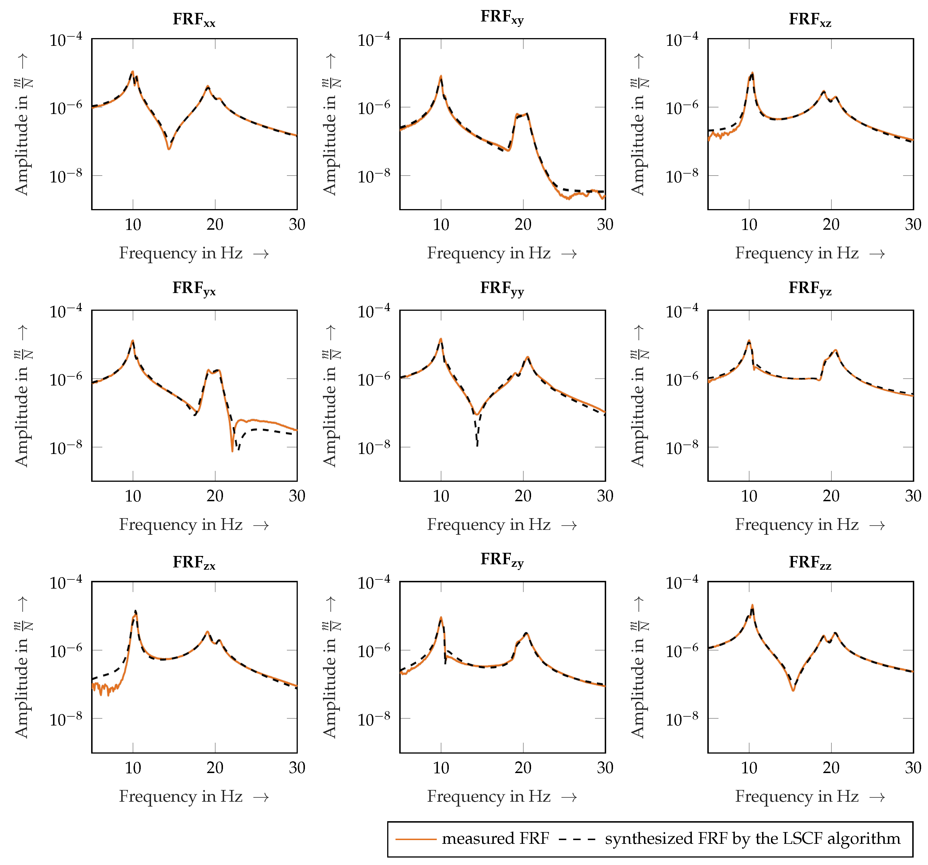
3.4. Reconstruction of Frequency Response Functions
3.5. Implementation Details
4. Discussion
5. Conclusions
- First, an information fusion approach to model the robot’s position-dependent natural frequencies improves the prediction accuracy significantly in comparison to that of conventional Gaussian process regression techniques, especially in scenarios with only a very small number of training data points. In those cases, the prediction uncertainty of conventional Gaussian processes is unreliable, whereas the uncertainty estimation of the linear information fusion scheme is reliable.
- Second, a detailed study was conducted to evaluate different kernel design choices for modeling the robot’s damping ratios and mode residues using conventional Gaussian process regression methods. The data analysis of the position-dependent damping ratios motivates the use of cubic kernels, whereas an RBF kernel is best suited for modeling the residues.
- Third, the position-dependent models can be used to estimate the position-dependent directional dynamics of the robot accurately and quantify the combined model uncertainty using a Monte Carlo algorithm.
Author Contributions
Funding
Institutional Review Board Statement
Informed Consent Statement
Conflicts of Interest
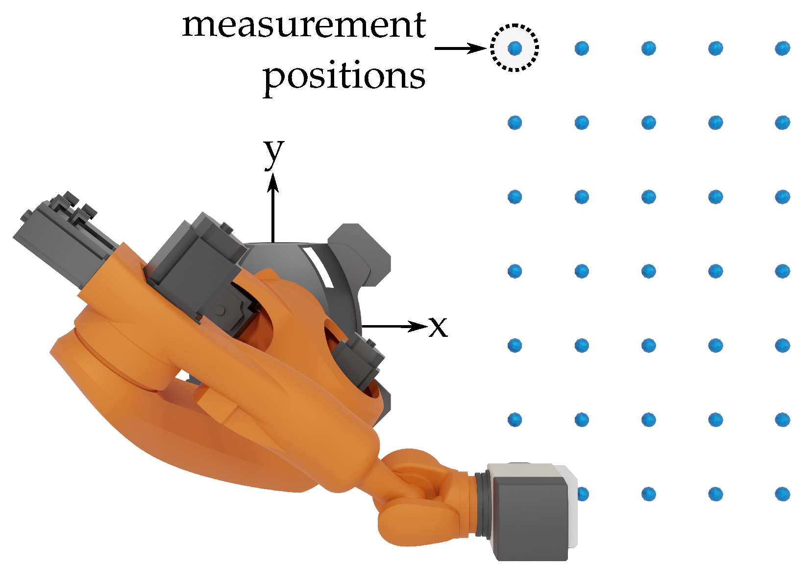
Appendix A. Measurement Locations

| x in m | y in m | z in m |
|---|---|---|
| 1.175 | −0.250 | 1.240 |
| 1.175 | −0.500 | 1.240 |
| 1.175 | 0.0 | 1.240 |
| 1.175 | 1.000 | 1.240 |
| 1.175 | 0.250 | 1.240 |
| 1.175 | 0.500 | 1.240 |
| 1.175 | 0.750 | 1.240 |
| 1.400 | −0.250 | 1.240 |
| 1.400 | −0.500 | 1.240 |
| 1.400 | 0.0 | 1.240 |
| 1.400 | 1.000 | 1.240 |
| 1.400 | 250 | 1.240 |
| 1.400 | 500 | 1.240 |
| 1.400 | 750 | 1.240 |
| 1.625 | −250 | 1.240 |
| 1.625 | −500 | 1.240 |
| 1.625 | 0.0 | 1.240 |
| 1.625 | 1.000 | 1.240 |
| 1.625 | 0.250 | 1.240 |
| 1.625 | 0.500 | 1.240 |
| 1.625 | 0.750 | 1.240 |
| 1.850 | −0.250 | 1.240 |
| 1.850 | −0.500 | 1.240 |
| 1.850 | 0.0 | 1.240 |
| 1.850 | 1.000 | 1.240 |
| 1.850 | 0.250 | 1.240 |
| 1.850 | 0.500 | 1.240 |
| 1.850 | 0.750 | 1.240 |
| 0.950 | −0.250 | 1.240 |
| 0.950 | −0.500 | 1.240 |
| 0.950 | 0.0 | 1.240 |
| 0.950 | 1.000 | 1.240 |
| 0.950 | 0.250 | 1.240 |
| 0.950 | 0.500 | 1.240 |
| 0.950 | 0.750 | 1.240 |
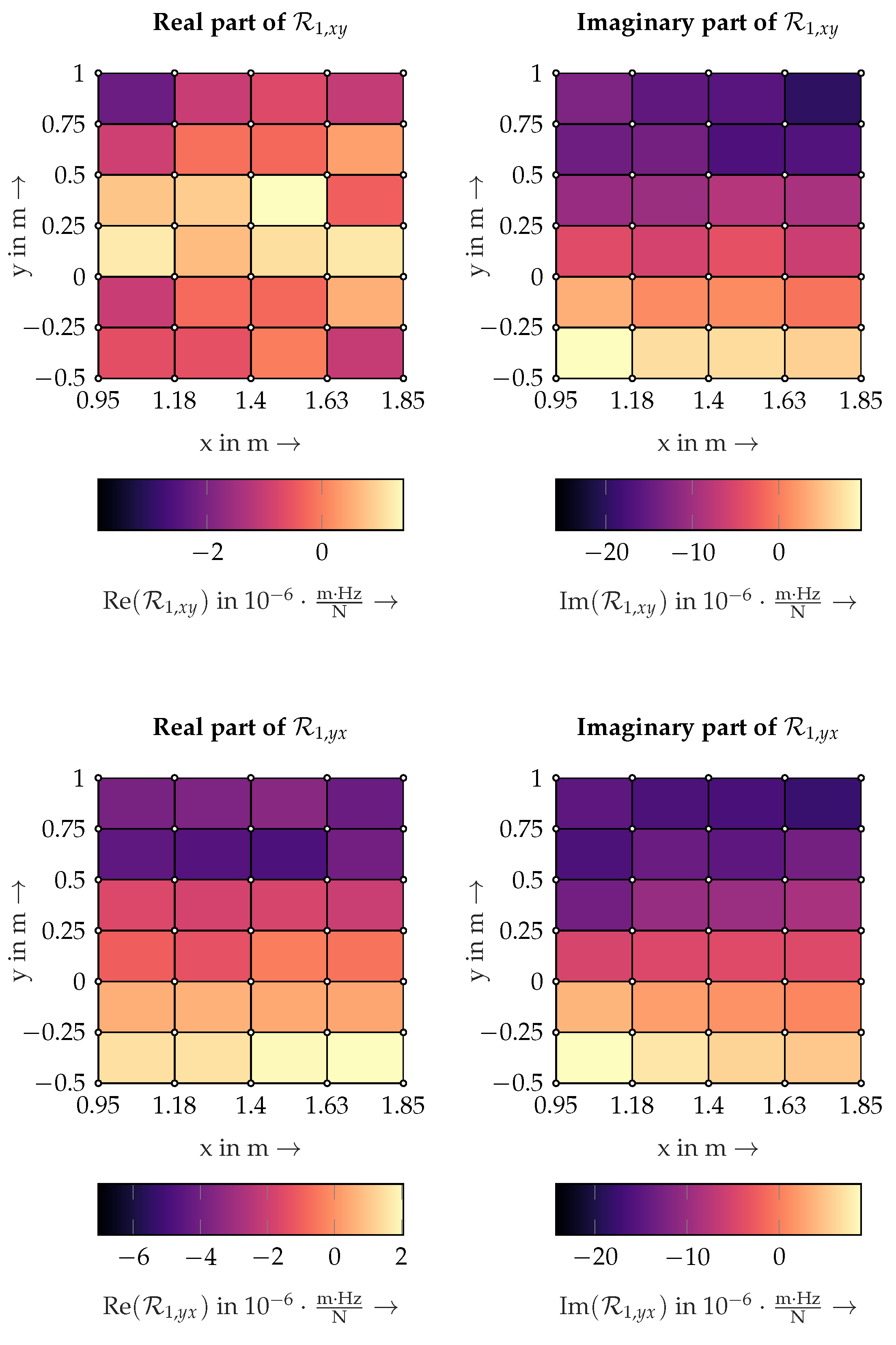
Appendix B. Cross Residuals Ri,xy and Ri,yx
Appendix C. Rigid Body Model of the Milling Robot
 = x,
= x,  = y,
= y,  = z.)
= x, = y, = z.)
= z.)
= x, = y, = z.)
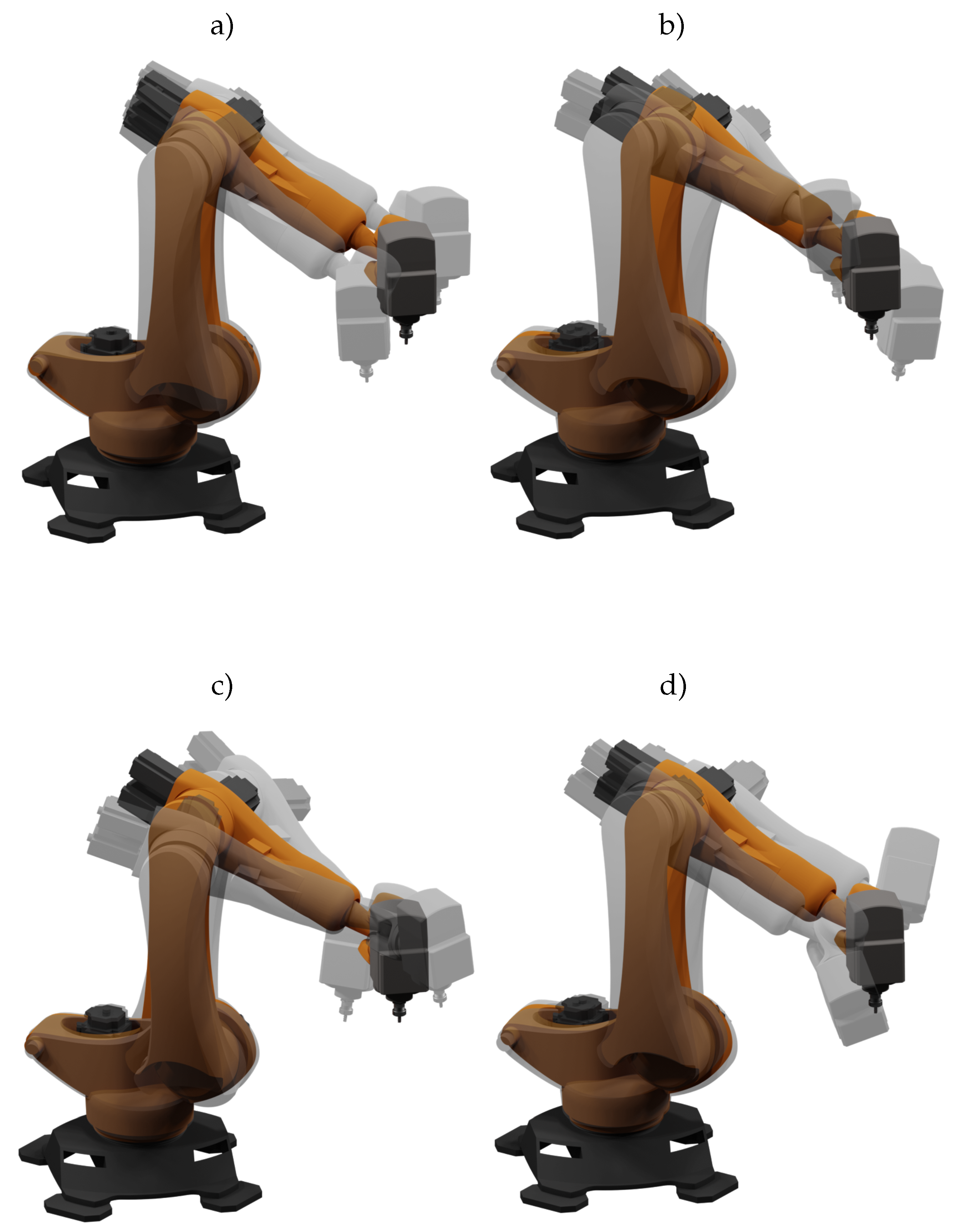
Appendix D. Mode Shape Visualization
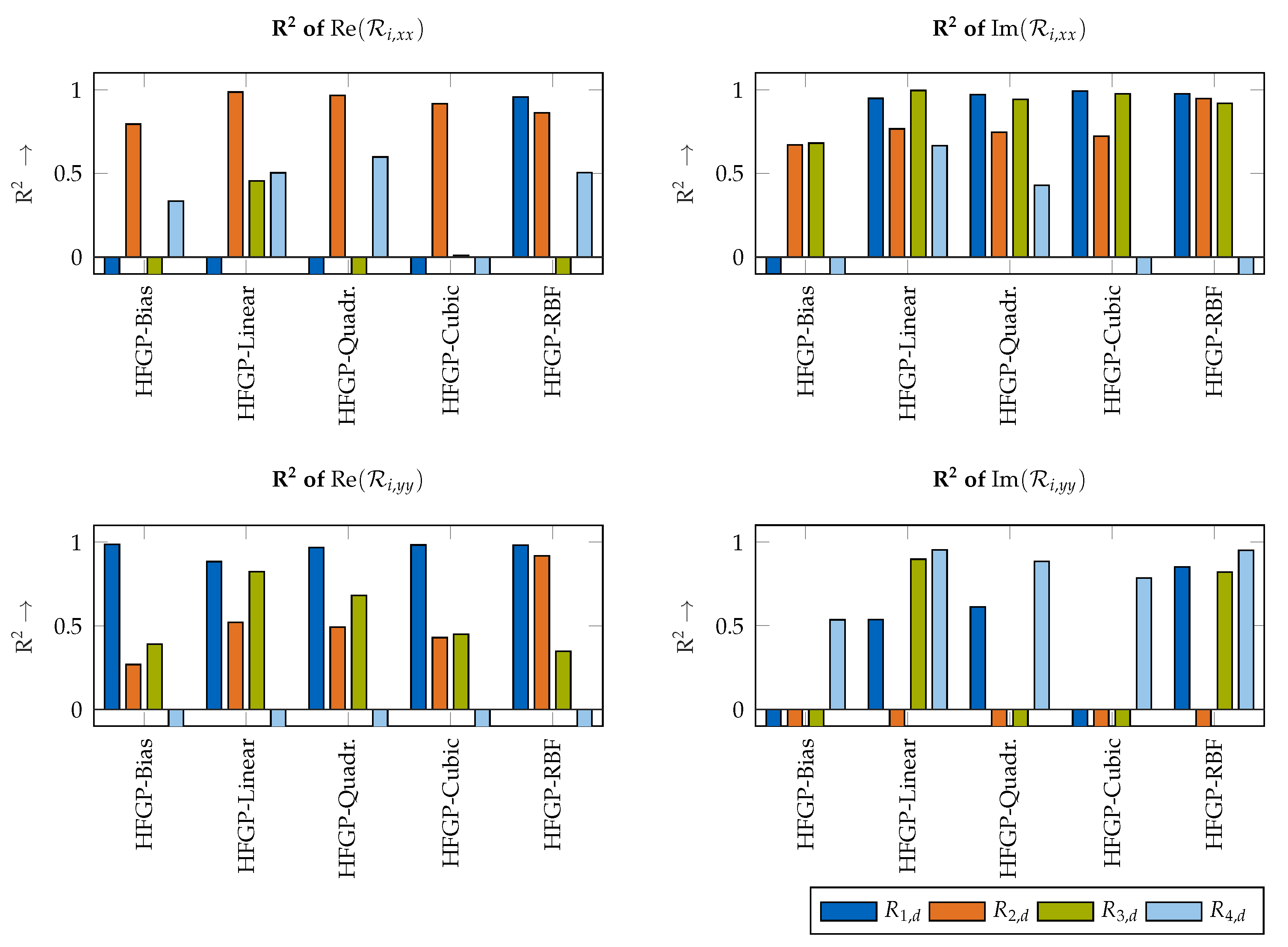
Appendix E. R2 results of Ri,xx and Ri,yy
References
- European Commission. The European Green Deal; European Commission: Brussels, Belgium, 2019. [Google Scholar]
- Baier, D.; Bachmann, A.; Zaeh, M.F. Towards wire and arc additive manufacturing of high-quality parts. Procedia CIRP 2020, 95, 54–59. [Google Scholar] [CrossRef]
- Fuchs, C.; Baier, D.; Semm, T.; Zaeh, M.F. Determining the machining allowance for WAAM parts. Prod. Eng. 2020, 14, 629–637. [Google Scholar] [CrossRef]
- Iglesias, I.; Sebastián, M.A.; Ares, J.E. Overview of the State of Robotic Machining: Current Situation and Future Potential. Procedia Eng. 2015, 132, 911–917. [Google Scholar] [CrossRef] [Green Version]
- Ji, W.; Wang, L. Industrial robotic machining: A review. Int. J. Adv. Manuf. Technol. 2019, 103, 1239–1255. [Google Scholar] [CrossRef] [Green Version]
- Karim, A.; Verl, A. Challenges and obstacles in robot-machining. In Proceedings of the 2013 44th International Symposium on Robotics, ISR 2013, Seoul, Korea, 24–26 October 2013. [Google Scholar]
- Rösch, O. Steigerung der Arbeitsgenauigkeit bei der Fräsbearbeitung Metallischer Werkstoffe mit Industrierobotern. Ph.D. Thesis, Technische Universität München, München, Germany, 2014. [Google Scholar]
- Zaeh, M.; Schnoes, F.; Obst, B.; Hartmann, D. Combined offline simulation and online adaptation approach for the accuracy improvement of milling robots. CIRP Ann. 2020, 69, 337–340. [Google Scholar] [CrossRef]
- Huynh, H.N.; Assadi, H.; Rivière-Lorphèvre, E.; Verlinden, O.; Ahmadi, K. Modelling the dynamics of industrial robots for milling operations. Robot.-Comput.-Integr. Manuf. 2020, 61, 101852. [Google Scholar] [CrossRef]
- Abele, E.; Rothenbücher, S.; Weigold, M. Cartesian compliance model for industrial robots using virtual joints. Prod. Eng. 2008, 2, 339–343. [Google Scholar] [CrossRef]
- Huynh, H.N.; Rivière-Lorphèvre, E.; Verlinden, O. Report of Robotic Machining Measurements Using a Stäubli TX200 Robot: Application to Milling. Volume 5B: 41st Mechanisms and Robotics Conference; American Society of Mechanical Engineers: New York, NY, USA, 2017; Volume 5B-2017. [Google Scholar]
- Dumas, C.; Caro, S.; Garnier, S.; Furet, B. Joint stiffness identification of six-revolute industrial serial robots. Robot.-Comput.-Integr. Manuf. 2011, 27, 881–888. [Google Scholar] [CrossRef] [Green Version]
- Busch, M.; Schnoes, F.; Elsharkawy, A.; Zaeh, M.F. Methodology for model-based uncertainty quantification of the vibrational properties of machining robots. Robot.-Comput.-Integr. Manuf. 2022, 73, 102243. [Google Scholar] [CrossRef]
- Nguyen, V.; Cvitanic, T.; Melkote, S. Data-Driven Modeling of the Modal Properties of a Six-Degrees-of-Freedom Industrial Robot and Its Application to Robotic Milling. J. Manuf. Sci. Eng. 2019, 141, 121006. [Google Scholar] [CrossRef]
- Nguyen, V.; Johnson, J.; Melkote, S. Active vibration suppression in robotic milling using optimal control. Int. J. Mach. Tools Manuf. 2020, 152, 103541. [Google Scholar] [CrossRef]
- Busch, M.; Schnoes, F.; Semm, T.; Zaeh, M.F.; Obst, B.; Hartmann, D. Probabilistic information fusion to model the pose-dependent dynamics of milling robots. Prod. Eng. 2020, 14, 435–444. [Google Scholar] [CrossRef]
- Peherstorfer, B.; Willcox, K.; Gunzburger, M. Survey of multifidelity methods in uncertainty propagation, inference, and optimization. arXiv 2018, arXiv:1806.10761. [Google Scholar] [CrossRef]
- Fernández-Godino, M.G.; Park, C.; Kim, N.H.; Haftka, R.T. Review of multifidelity models. arXiv 2016, arXiv:1609.07196. [Google Scholar]
- Liu, Y.P.; Altintas, Y. Predicting the position-dependent dynamics of machine tools using progressive network. Precis. Eng. 2022, 73, 409–422. [Google Scholar] [CrossRef]
- Verboven, P. Frequency-Domain System Identification for Modal Analysis. Ph.D. Thesis, Vrije Universiteit Brussel, Brussel, Belgium, 2002. [Google Scholar]
- Puzik, A. Genauigkeitssteigerung bei der Spanenden Bearbeitung mit Industrie- robotern durch Fehlerkompensation mit 3D-Piezo-Ausgleichsaktorik. Ph.D. Thesis, Universität Stuttgart, Stuttgart, Germany, 2011. [Google Scholar]
- Geradin, M.; Rixen, D.J. Mechanical Vibrations: Theory and Application to Structural Dynamics, 3rd ed.; John Wiley & Sons, Ltd.: Chichester, UK, 2015. [Google Scholar]
- Reinl, C.; Friedmann, M.; Bauer, J.; Pischan, M.; Abele, E.; Von Stryk, O. Model-based off-line compensation of path deviation for industrial robots in milling applications. In Proceedings of the IEEE/ASME International Conference on Advanced Intelligent Mechatronics, AIM, Budapest, Hungary, 3–7 July 2011; pp. 367–372. [Google Scholar]
- Kennedy, M.C.; O’Hagan, A. Predicting the output from a complex computer code when fast approximations are available. Biometrika 2000, 87, 1–13. [Google Scholar] [CrossRef] [Green Version]
- Perdikaris, P.; Raissi, M.; Damianou, A.; Lawrence, N.D.; Karniadakis, G.E. Nonlinear information fusion algorithms for robust multi-fidelity modeling. Proc. R. Soc. Math. Phys. Eng. Sci. 2016, 473, 751. [Google Scholar]
- Rasmussen, C.E.; Williams, C.K.I. Gaussian Processes for Machine Learning. Int. J. Neural Syst. 2006, 11, 3011–3015. [Google Scholar]
- Lemieux, C. Monte Carlo and Quasi-Monte Carlo Sampling; Springer Series in Statistics; Springer: New York, NY, USA, 2009. [Google Scholar] [CrossRef] [Green Version]
- Tennøe, S.; Halnes, G.; Einevoll, G.T. Uncertainpy: A Python Toolbox for Uncertainty Quantification and Sensitivity Analysis in Computational Neuroscience. Front. Neuroinform. 2018, 12, 1–29. [Google Scholar] [CrossRef] [PubMed] [Green Version]
- Zaletelj, K.; Bregar, T.; Gorjup, D.; Slavič, J. pyEMA. 2020. Available online: https://github.com/ladisk/pyEMA (accessed on 20 January 2022).
- Felis, M.L. RBDL: An efficient rigid-body dynamics library using recursive algorithms. Auton. Robot. 2017, 41, 495–511. [Google Scholar] [CrossRef]
- Sheffield Machine Learning Software. GPy: A Gaussian Process Framework in Python. 2012. Available online: http://github.com/SheffieldML/GPy (accessed on 20 January 2022).
- Paleyes, A.; Pullin, M.; Mahsereci, M.; Lawrence, N.; González, J. Emulation of physical processes with Emukit. In Proceedings of the Second Workshop on Machine Learning and the Physical Sciences, NeurIPS, Vancouver, BC, Canada, 8–14 December 2019. [Google Scholar]
- Busch, M.; Schmucker, B.; Zaeh, M.F. Rapid uncertainty quantification of the stability analysis using a probabilistic estimation of the process force parameters. MM Sci. J. 2021, 2021, 4978–4983. [Google Scholar] [CrossRef]
- Lau, J.; Lanslots, J.; Peeters, B.; Van Der Auweraer, H. Automatic modal analysis: Reality or myth? In Proceedings of the IMAC 25, Orlando, FL, USA, 19–22 February 2007. [Google Scholar]


| Purpose | Package | Version | Language |
|---|---|---|---|
| Data acquisition | Data acquisition toolbox | R2021a | Matlab |
| Generation of frequency domain data | Signal processing toolbox | R2021a | Matlab |
| Experimental modal analysis | pyEMA [29] | 0.23 | Python |
| (Maximin) LHS sampling | scikit-optimize | 0.8.1 | Python |
| Rigid body model | RBDL (ORB Version) [30] | 3.0.0 | C++/Python |
| HFGP models | GPy [31] | 1.9.9 | Python |
| AR1 model | emukit [32] | 0.4.8 | Python |
| NARGP model | emukit [32] | 0.4.8 | Python |
| Monte Carlo simulation | Uncertainpy [28] | 1.2.3 | Python |
Publisher’s Note: MDPI stays neutral with regard to jurisdictional claims in published maps and institutional affiliations. |
© 2022 by the authors. Licensee MDPI, Basel, Switzerland. This article is an open access article distributed under the terms and conditions of the Creative Commons Attribution (CC BY) license (https://creativecommons.org/licenses/by/4.0/).
Share and Cite
Busch, M.; Zaeh, M.F. Multi-Fidelity Information Fusion to Model the Position-Dependent Modal Properties of Milling Robots. Robotics 2022, 11, 17. https://doi.org/10.3390/robotics11010017
Busch M, Zaeh MF. Multi-Fidelity Information Fusion to Model the Position-Dependent Modal Properties of Milling Robots. Robotics. 2022; 11(1):17. https://doi.org/10.3390/robotics11010017
Chicago/Turabian StyleBusch, Maximilian, and Michael F. Zaeh. 2022. "Multi-Fidelity Information Fusion to Model the Position-Dependent Modal Properties of Milling Robots" Robotics 11, no. 1: 17. https://doi.org/10.3390/robotics11010017
APA StyleBusch, M., & Zaeh, M. F. (2022). Multi-Fidelity Information Fusion to Model the Position-Dependent Modal Properties of Milling Robots. Robotics, 11(1), 17. https://doi.org/10.3390/robotics11010017