Abstract
Robotic machining is a promising technology for post-processing large additively manufactured parts. However, the applicability and efficiency of robot-based machining processes are restricted by dynamic instabilities (e.g., due to external excitation or regenerative chatter). To prevent such instabilities, the pose-dependent structural dynamics of the robot must be accurately modeled. To do so, a novel data-driven information fusion approach is proposed: the spatial behavior of the robot’s modal parameters is modeled in a horizontal plane using probabilistic machine learning techniques. A probabilistic formulation allows an estimation of the model uncertainties as well, which increases the model reliability and robustness. To increase the predictive performance, an information fusion scheme is leveraged: information from a rigid body model of the fundamental behavior of the robot’s structural dynamics is fused with a limited number of estimated modal properties from experimental modal analysis. The results indicate that such an approach enables a user-friendly and efficient modeling method and provides reliable predictions of the directional robot dynamics within a large modeling domain.
1. Introduction
To achieve the climate targets set by the European Commission, formulated in the The European Green Deal in 2019 [1], modern production processes must continuously become more energy and resource-efficient. In the aerospace industry especially, where the production of large structural components is resource-intensive, additive manufacturing processes promise high resource efficiency [2]. Nevertheless, post-processing of the workpieces, for example by milling, is still required to achieve high geometrical accuracy [3].
In such scenarios, machining robots are the ideal platforms to follow the additive manufacturing processes in the process chain, because they offer a large workspace and at the same time low investment costs compared to conventional machine tools [4,5]. However, their low dynamic stiffness continues to limit their industrial application [6,7,8]. On the one hand, forced vibrations (e.g., when a tooth passing frequency coincides with a robot’s natural frequency) can cause significant damage to the tool and spindle components. On the other hand, self-excited regenerative chatter can limit the depth of cut and therefore reduce the robot’s efficiency because of a limited material removal rate. Additionally, unstable machining processes result in poor surface quality of the workpiece.
Hence, modeling the (pose-dependent) vibrational properties of machining robots is of high interest. In this work, a novel data-driven approach for modeling the pose-dependent dynamics of milling robots is presented.
1.1. Related Work
In recent years, various methods for modeling the pose-dependent vibrational properties of machining robots have been proposed. Roughly, the proposed approaches can be divided into classical physics-based methods and data-driven algorithms:
Physics-based methods
Physics-based models are based on classical mechanistic modeling techniques, such as
- conventional rigid-body models [9],
- rigid-body models with additional virtual joints [10] or
- finite element models [11].
Mostly, these models can be formulated in the following form:
The model’s generalized coordinates represent the rotational degrees of freedom of the robot joints. The pose-dependent mass matrix consists of the robot bodies’ mass and inertia properties, while the system’s damping and stiffness matrices and are usually considered to be pose-independent. Lastly, are the resulting torques around the model’s degrees of freedom.
As presented by Huynh et al. [9], the modeling accuracy of the vibrational behavior can be significantly improved, if not only includes the actuated degrees of freedom around the actuated axes, but also tilting rotations (resulting in three rotational degrees of freedom for each physical robot joint). However, the parameter identification process for the model parameters in , and remains an open issue, because conventional parameter identification procedures often result in physically infeasible parameters and, thus, should only be treated as fitting parameters [9]. Based on the popular approach of Dumas et al. [12], Busch et al. [13] presented a methodology to infer physically feasible compliance parameters using a Bayesian regression approach. Additionally, Huynh et al. [9] proposed a methodology to estimate the model’s mass and inertia properties.
However, all physics-based approaches rely on complex experimental designs, cost-intensive measurement technology (such as dynamometers and laser trackers), and mathematically advanced identification schemes to estimate the pose-dependent dynamics accurately, which prevent industrial applications.
Data-driven algorithms
In contrast to physics-based methods, recent works aimed at deriving the pose-dependent dynamics of machining robots solely from data. The use of modern machine learning algorithms promises a simpler and more efficient system modeling approach [14]. Furthermore, when probabilistic algorithms such as Gaussian process regression techniques are used, the resulting data-driven models can take reliable uncertainty measures into account. For example, Nguyen et al. [14] proposed a data-driven approach using Gaussian process regression to model the robot’s position-dependent modal properties (natural frequency, damping ratio and dynamic stiffness). Based on such a model, an active vibration suppression controller was developed [15].
However, conventional data-driven modeling techniques usually require expert knowledge during the algorithm setup. Typically for conventional Gaussian process models, the underlying covariance function and the noise model must be carefully chosen and designed based on domain knowledge. If the algorithm’s hyperparameters (such as the covariance function) are not well designed, the data-driven models cannot predict the robot’s dynamics accurately.
1.2. Motivation
Summarizing, a precise and yet efficient modeling technique for the pose-dependent vibrational dynamics remains an open issue, even though multiple approaches provide methods to model the dynamics with different levels of fidelity and model efficiency.
As shown in previous works, the problem at hand motivates the application of so-called multi-fidelity information fusion schemes [16]. Such algorithms are especially appealing, when multiple information sources with different levels of information quality are available [17,18]. Typically for general dynamical systems, there are multiple approaches for modeling a system’s dynamic behavior, each with a different level of fidelity. Information fusion schemes can take advantage of the linear or even nonlinear relationship between the two or more information sources. Hence, these algorithms can reduce the burden of evaluating the high fidelity model for all system states of interest, by exploiting the fact that the low-fidelity model already contains a rough estimate.
Regarding the given issue, analytical structural models of an industrial machining robot can provide essential information on the underlying system dynamics (even though their accuracy in respect of the positional vibration properties might be limited), while a limited number of experimental data samples will provide precise information on the actual system behavior. An information fusion scheme allows to model the spatial system dynamics by fusing both information sources [16]. However, the previously proposed method is based on frequency domain data. As Gaussian process regression algorithms scale poorly with the number of data points, the proposed methodology was limited by the number of data samples.
The idea of fusing this kind of information was recently adopted by Liu and Altintas [19], who proposed a transfer learning scheme using artificial neural networks to model the pose-dependent dynamics of conventional machine tools.
1.3. Scope and Approach
Based on the works of Nguyen et al. [14] and Busch et al. [16], a novel methodology for modeling the position-dependent modal properties of a machining robot is proposed in the following sections: based on a multi-fidelity scheme, a precise model of the robot’s vibrational properties is developed. An existing, but imprecise analytical robot model provides low-fidelity information, whereas experimental modal analysis (EMA) experiments provide accurate high-fidelity data.
As the spatial (i.e., position-dependent) model of the robot’s natural frequencies is the key component for predicting whether a machining process will be stable or to suppress vibrations using active vibration control, the natural frequencies are the key focus of this paper and are therefore considered as a primary feature.
To evaluate the vibrational behavior at any location in the workspace, the damping ratios and mode shape vectors (if physically scaled, these are also called residues) are also of interest, for example to reconstruct the position-based frequency response function. Hence, those two features are considered to be secondary features.
2. Methods
The presented methodology aims at generating probabilistic models of the vibrational properties of machining robots. For this purpose, the spatial vibrational behavior of such a machining robot is represented by the following three modal properties of the robot’s structure, depending on the workspace position in a horizontal plane ():
- the natural frequencies for each vibration mode of the robot structure,
- the damping ratios for each vibration mode of the robotstructure and
- the residues for each vibration mode and in each mode direction .
To model the spatial behavior of the robot’s natural frequencies accurately, two probabilistic information fusion schemes are presented and benchmarked against a conventional approach.
Therefore, the outline of the methodology is as follows:
- Data generation: first, the modal parameters are derived from the analytical model and gathered experimentally at the robot (see Section 2.1).
- Data preparation: the data sets are divided into training and testing data sets (see Section 2.2).
- Model setup and training: the spatial behavior of the vibrational features is modeled as follows (see Section 2.3):
- (a)
- The primary features (natural frequencies) are modeled using multi-fidelity information fusion approaches (see Section 2.3.1).
- (b)
- The secondary features (damping ratios and residues) are modeled using conventional Gaussian process regression techniques (see Section 2.3.2 and Section 2.3.3).
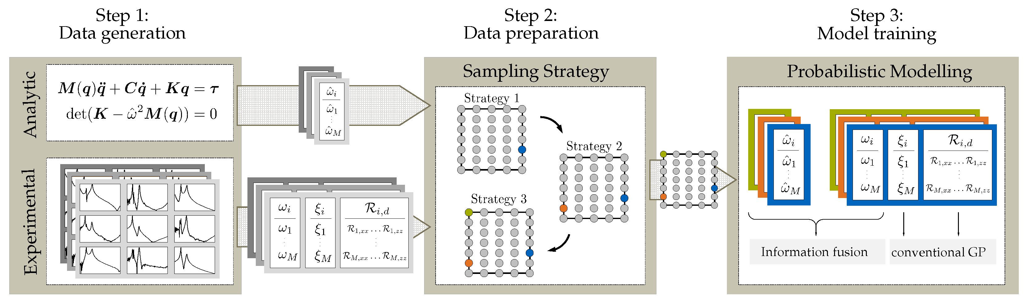
The methodology is illustrated in Figure 1.
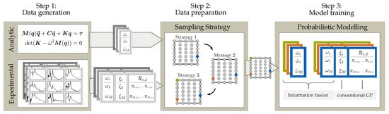
Figure 1.
Methodology of the approach.
2.1. Data Generation: Spatial Modal Parameter Identification
All of the following investigations and experiments were conducted using a Kuka kr240 R2500 prime robot. The robot is equipped with a high-speed milling spindle from Helmuth Diebold GmbH & Co., Jungingen, Germany (type HSG-E 198.18-38 AK1). All the following coordinates are referenced to the robot’s base coordinate system.
To obtain experimental training and testing data, impact hammer tests were conducted for 35 robot configurations in the x-y-plane at a constant height z of 1.24 m with a constant TCP orientation, followed by the estimation of the modal properties using the Least-Squares Complex Frequency Domain (LSCF) algorithm [20]. The measurement locations are illustrated in Figure 2. The coordinates are given in the Appendix A (see Table A1).
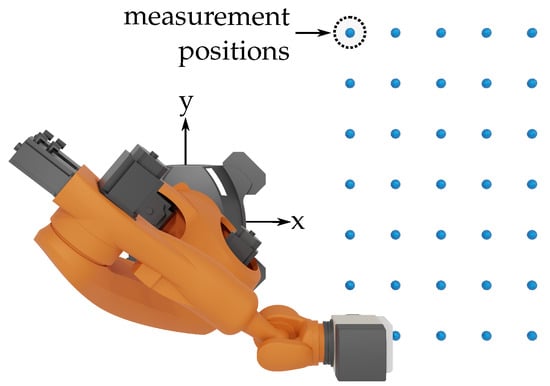
Figure 2.
Measurement positions in the workspace of the robot and the base coordinate system.
A Kistler impact hammer (type 9728A20000, force range up to 20 kN) and a Kistler 3D-accelerometer (type 8762A50) were used. The accelerometer was placed on the spindle. The excitations created by the impact hammer were made in each spatial direction (x-, y- and z-direction) and performed 10 times each to reduce the measurement noise and nonlinear effects. As described by Puzik [21] and Huynh et al. [9], the effect of the active motor controller is negligible. Therefore, the measurements were performed with brakes engaged.
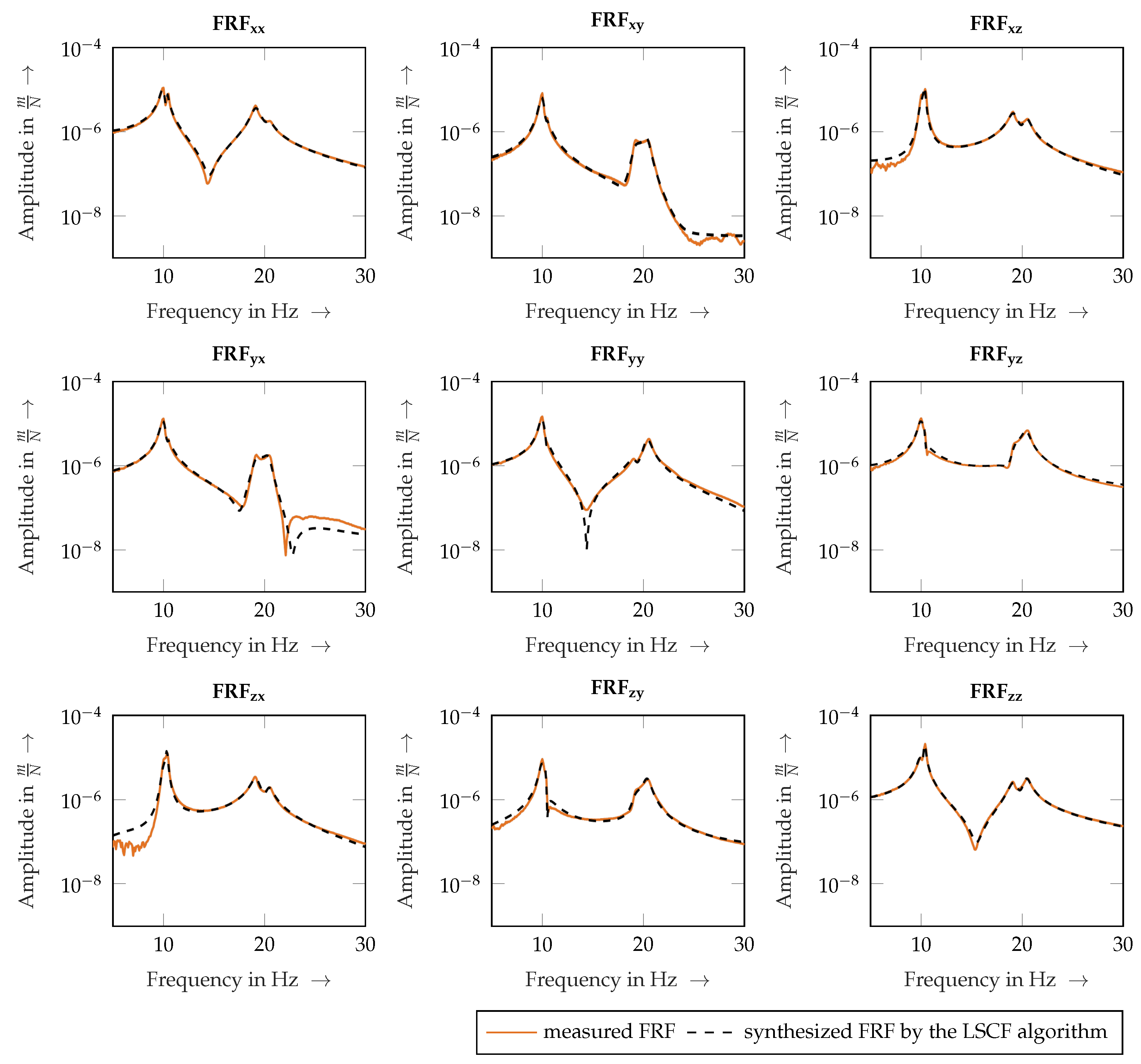
The measured directional frequency response functions (FRFs) at the point and the corresponding synthesized FRFs based on the estimated modal parameters of the LSCF algorithm are displayed in Figure 3.
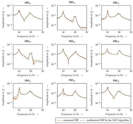
Figure 3.
Measured directional frequency response functions and synthesized estimation by Least-Squares Complex Frequency Domain (LSCF) algorithm.
To visualize the spatial behavior of the robot’s vibrational properties, the modal parameters of the first vibration mode are illustrated in Figure 4. For simplicity, only the spatial behavior of the direct residues in the x- and y-directions, and , are shown. Illustrations of the cross residuals and are given in the Appendix B (see Figure A1).
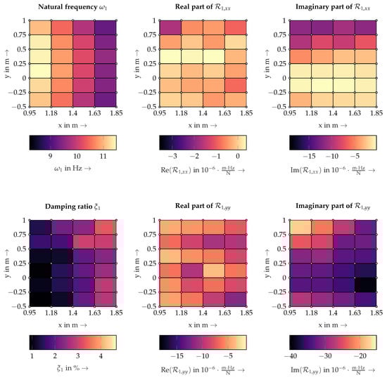
Figure 4.
Spatial behavior of modal parameters of first vibration mode.
As illustrated, the natural frequency changes continuously depending on the tool center point’s position: decreases, as the tool center point (TCP) moves away from the robot’s base.
Roughly, the damping ratio increases with increasing distance of the TCP to the robot’s base, even though clear spatial behavior is not apparent in the data.
The imaginary part of decreases approximately linearly in the y-direction and is approximately constant in the x-direction, while the imaginary part of decreases with increasing x-direction but increases with increasing y-direction. The real parts of and are significantly smaller than their respective imaginary parts (indicating a rather lightly damped structure), but also significantly noisier.
2.2. Data Preparation: Sampling Methodology
To train and test the probabilistic models, the split into training and testing data must be carefully chosen: the training data must include as much information on the spatial behavior as possible and enough testing data points must be included to ensure the validity of the predicted model behavior.
The sampling methodology applied in this study involves two steps:
In a first step, the general validity of the approach is demonstrated using 15 training data points (and 20 testing data points , respectively). In the following section, this training and testing split is referred to as sampling strategy A.
To do so, conventional sampling techniques, such as Latin-Hypercube-Sampling (LHS) or Sobol-Sampling, can be used. In the following, the application of an LHS approach is described: first, the division into and is performed using an adapted LHS technique in the robot’s workspace (i.e., an LHS approach and maximizing the minimum distance between all points).
In a second step, the sensitivity of the model accuracy to the number of training data points is investigated. Hence, this will investigate how an increasing number of training data points improves the modeling accuracy. The following sampling approach is referred to as sampling strategy .
Depending on the desired number of data points in the actual training data set, random samples are taken iteratively from . Hence, the actually used training data set is sampled in each iteration into and , conditional upon
To ensure the comparability between the results, the following principles are taken into account for sampling the training data set in each iteration:
- The testing data set remains the same for all investigations.
- The actually used training data points are subsampled from the original training data set .
Figure 5 illustrates the training and testing locations for the sampling strategy A and for 3, 5, 7, and 10 training data points in the sampling strategy B. It is worth noting, that for 15 training data points, the sampling strategy equals the sampling strategy A.
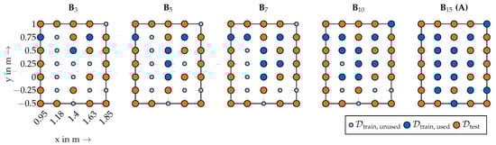
Figure 5.
Training and testing data points for sampling strategies , , , and (A).
2.3. Model Setup and Training: Data Driven Modeling of the Modal Properties
The following three sections present new approaches to model the spatial behavior of the robot’s
- natural frequencies (Section 2.3.1),
- damping ratios (Section 2.3.2) and
- residues (Section 2.3.3).
2.3.1. Primary Feature: Natural Frequencies
As presented in Section 1, the concept of multi-fidelity information fusion shall be transferred to modeling of the spatial behavior of the robot’s natural frequencies: the low-fidelity information is provided by the rigid body model of the robot. Based on the model’s mass and stiffness matrices and , the position-dependent natural frequencies are the eigenvalues of the system’s eigenvalue problem [22]:
Instead of a computer model with higher fidelity, the high-fidelity information is represented by the experimentally estimated natural frequencies of the robot’s structure at different workspace positions (see Section 2.1).
In this respect, Figure 6 illustrates the spatial behavior of the measured natural frequencies in comparison to the estimated natural frequencies by a rigid body simulation.
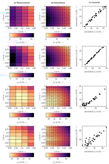
Figure 6.
Spatial behavior of first natural frequency as measured (column a)) and predicted by simulation (column b)). There is a linear dependency between simulation results and measurements (column c)).
For simplicity, the rigid body model is equivalent to the model published in [16]. The definition of the rigid body model and its parameters are given in the Appendix C (see Figure A2). The mass and inertia properties of the bodies were estimated using the CAD model of robot, similar to the approach of Reinl et al. [23]. The joint stiffness values were taken from the previous works by Rösch [7]. Additionally, illustrations of the first four mode shapes are given in the Appendix D as well (see Figure A3).
As shown, a rather linear relationship exists between the rigid body simulation () and the experimentally estimated natural frequency (). However, depending on the accuracy of the rigid body model, this relationship is not necessarily linear.
In the following, two approaches to inferring the relationship between the low fidelity simulation and the high fidelity measurement data are used and compared: the linear auto-regressive scheme (AR1), which was proposed by Kennedy and O’Hagan [24] can estimate a linear relationship, whereas the nonlinear auto-regressive multi-fidelity gp (NARGP) by Perdikaris et al. [25] is even able to model nonlinear relationships. Both approaches rely on Gaussian process regression techniques, which incorporate prior beliefs about the underlying system dynamics by choosing appropriate kernel functions. Furthermore, since Gaussian processes are Bayesian machine learning techniques, they provide reliable uncertainty estimates of their predictions.
To illustrate the strengths of the proposed approach, the two multi-fidelity algorithms are benchmarked against regular Gaussian process techniques using only the high fidelity measurement data (abbreviated below as HFGP). Following the kernel definitions of Rasmussen and Williams [26], different kernel design choices for a regular Gaussian process setup are evaluated:
- a linear kernel: a linear kernel makes it possible to incorporate a linear spatial model using the variance :
- a quadratic kernel: a quadratic kernel allows more flexibility than a simple linear kernel and is represented by
- a cubic kernel: similar to the generation of a quadratic kernel, the idea of a polynomial kernel can be extended to a cubic kernel, given by
- a radial basis function (RBF) kernel: the conventional RBF kernel is a very popular kernel, as no assumption on the data’s structure is incorporated. However, an RBF kernel may be prone to overfitting. The kernel is defined aswhere is the variance and l is the lengthscale of the RBF kernel.
Furthermore, the data are normalized before the training procedure. The hyperparameters of each model are optimized during training using five optimization runs.
The three approaches (HFGP, AR1 and NARGP) are validated and benchmarked against each other in Section 3.1.
2.3.2. Secondary Feature: Damping Ratios
Numerous research publications relating to modeling of the spatial dynamic behavior of machining systems indicate that modeling the damping effects of robots and machine tools is inherently difficult: as shown by Nguyen et al., the damping ratios exhibit the least “correlation with position compared to natural frequencies and stiffness” [14]. Furthermore, a clear spatial behavior is not evident from the measurements as illustrated in Section 2.1. Hence, in the context of Gaussian process regression techniques, assuming no spatial behavior, the data distribution can simply be modeled by a constant bias kernel. Such a kernel is given by
In the event that a spatial behavior of the damping ratios is to be modeled, the previously mentioned kernels , , and can be chosen. Therefore, the performance of a constant bias kernel and of the spatial modelling kernels , , and will be evaluated and discussed in Section 3.2.
The hyperparameters are derived during training. Analogously to the natural frequencies, the data are normalized before training and the training consists of five optimization runs.
2.3.3. Secondary Feature: Residues
To predict the dynamic response of the robot structure accurately, information on the response amplitudes, represented by the structure’s mode shapes or residues, is also of interest. Both mode shapes and residues represent the same physical property of a dynamic vibration system. Their relationship can best be explained by considering the reconstruction of a frequency response function in direction d using the system’s natural frequencies and their corresponding damping decay rates and mode shapes :
with
are the complex poles of the system. The scaling of the mode shapes using the scaling factor yields the residues :
Hence, the residues represent the scaled vibration modes and can be derived directly from the LSCF algorithm during the modal parameter identification process (see Section 2.1).
Similar to the damping ratios, the spatial behavior of the robot’s modal residues can also be modeled using conventional Gaussian process regression. However, since residues are generally complex-valued, each residue is modeled using two independent Gaussian processes. Again, the performance of the presented kernels , , , and is compared in Section 3.3. Analogously to the natural frequencies and damping ratios, the hyperparameters are derived during training. The data are normalized before training and the training consists of five optimization runs.
3. Results
In the following three Section 3.1, Section 3.2 and Section 3.3, the modeling approaches for three modal parameters are individually validated. Then in Section 3.4, the performance of the presented spatial modeling approach is highlighted using the reconstruction capabilities of position-based frequency response functions. Implementation details are given in Section 3.5 for future reproducibility of the methodology.
3.1. Primary Feature: Natural Frequencies
As presented in Section 2.2, the approach to validating the spatial modeling of the natural frequencies proceeds in two steps: first, the different algorithms are benchmarked against each other in Section 3.1.1. Second, the accuracies of the three best-performing algorithms are assessed in Section 3.1.2, based on a varying number of training data points.
3.1.1. Validity of the Approach
To benchmark the three presented algorithms against each other, the 35 measurements are split into 15 training data points and 20 testing data points using the optimized LHS algorithm (see Section 2.2).
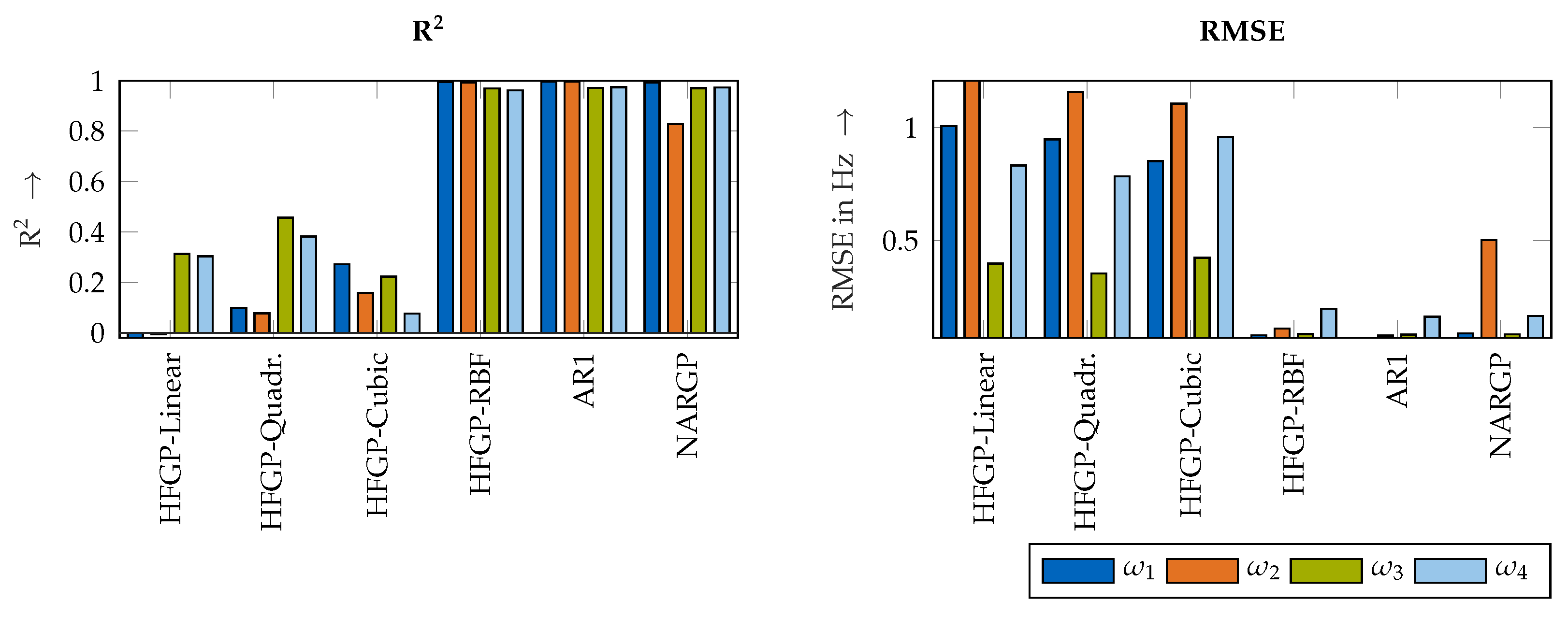
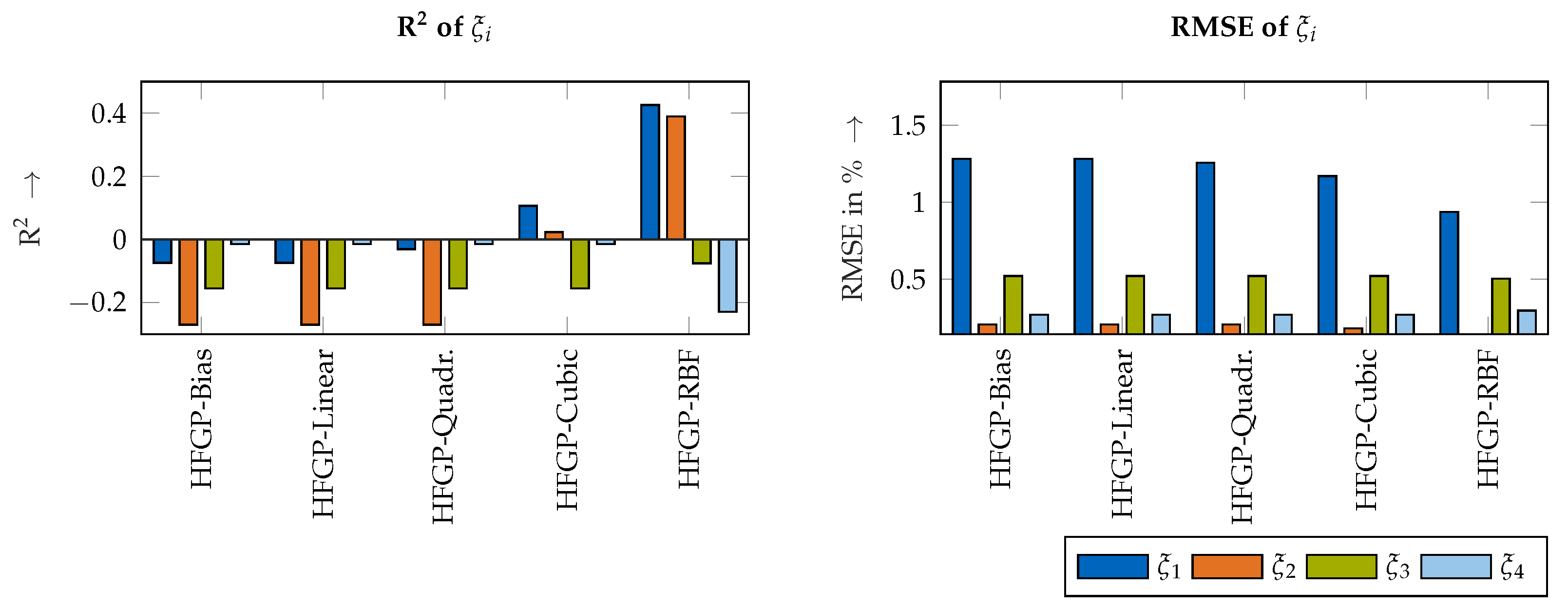
The performance of the four kernels for the Gaussian process regression and the two multi-fidelity algorithms (see Section 2.3.1) are rated according to the achieved coefficient of determination () and the root-mean-square error (RMSE), based on each model’s prediction of the testing data set. The results are illustrated separately in Figure 7 for each modeled natural frequency.

Figure 7.
Benchmark metrics for each model’s prediction at testing data points.
It is apparent that the spatial behavior of the natural frequencies cannot be modeled adequately using only the high-fidelity data in combination with a linear, quadratic, or cubic kernel: only low coefficients of determination are obtained, and the root-mean-square errors are large. In contrast, the conventional RBF kernel and the two multi-fidelity schemes yield comparably good results: the achieved coefficient of determination is mostly higher than 0.9, and their root-mean-square errors are significantly lower in comparison to that of the linear, quadratic, or cubic kernels.
Hence, all three modeling approaches (HFGP-RBF, AR1 and NARGP) can adequately capture the spatial behavior of the natural frequencies, provided enough training data are available throughout the workspace of interest.
3.1.2. Accuracy Using an Increasing Number of Training Data Points
The performance of the conventional Gaussian process with an RBF kernel, the linear AR1 model and the nonlinear NARGP model can be further benchmarked regarding the prediction accuracy with an iteratively increasing number of measurements. As described in Section 2.2, an LHS-based sampling strategy was used for 3 to 15 measurements.
Again, the model performance is evaluated using the achieved coefficient of determination and the resulting root-mean-square error RMSE. The results are illustrated in Figure 8. For a better comparison, a dashed horizontal line indicates the threshold .
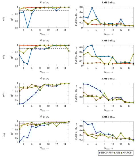
Figure 8.
Benchmark of conventional Gaussian process regression with an RBF kernel and the two multi-fidelity schemes AR1 and NARGP using iterative sampling of training data points.
It appears that both multi-fidelity information fusion algorithms perform notably better than the conventional Gaussian process with the RBF kernel, when only a small number of measurements is available.
However, the performance of the NARGP model is fluctuating, whereas the AR1 approaches and more quickly than the NARGP model with an increasing number of training points . This finding is supported by the assumption of a rather linear relationship between the rigid body model and the experimental data as indicated in Section 2.3.1. Hence, the linear multi-fidelity scheme AR1 enables a more efficient estimation of the spatial behavior of the robot’s eigenfrequencies, even when only a small number of training data points is available.
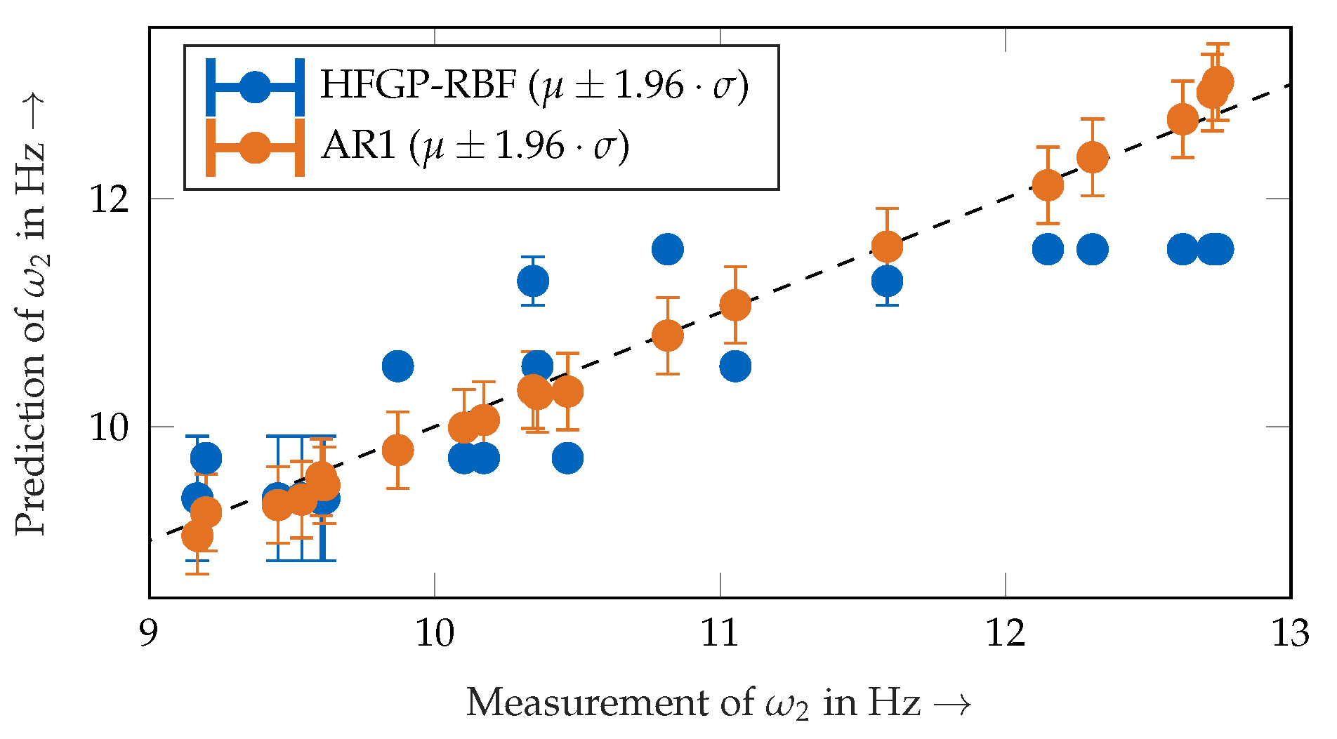
Lastly, since all models are based on Gaussian process regression techniques, they provide methods to evaluate the prediction uncertainty. To highlight the strength of the proposed multi-fidelity modeling scheme AR1, Figure 9 illustrates the model prediction and the confidence interval for the second natural frequency for only measurements used for training (i.e., the sampling strategy ). The AR1 algorithm models the spatial behavior of accurately and provides reliable uncertainty boundaries, whereas the predictions of the conventional Gaussian process using the RBF kernel are inaccurate and do not even provide reliable prediction intervals (the model predictions are overconfident).
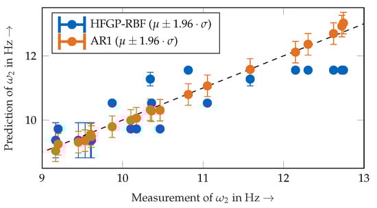
Figure 9.
Comparison of prediction accuracy on testing data of using sampling strategy , including model’s predictive uncertainty in form of the 95% prediction interval.
3.2. Secondary Feature: Damping Ratios
As explained in Section 2.3.2, regular Gaussian process models were set up to model the damping ratios with different kernel choices, namely , , , and .
Analogously to the analysis described in Section 3.1.1, the accuracy of the model prediction at the 20 testing data points using the 15 training data points is illustrated in Figure 10 using the coefficient of determination and the root-mean-square error RMSE.

Figure 10.
Benchmark between different kernel designs for modeling damping ratios.
It is apparent that the spatial modeling approach of the damping ratios performs significantly worse than the spatial modeling of the natural frequencies: the coefficient of determination indicates that none of the kernels can model the spatial behavior accurately, even though the model using the RBF kernel seems to capture the underlying spatial behavior best.
However, it is crucial to remember that the measured damping ratios themselves do not indicate a clear spatial behavior due to the inherent nonlinear damping dynamics, so every modeling approach will perform poorly with such noisy training data. Due to this fact, use of the RBF kernel is not advised, because the modeling performance can depend strongly on the measurement positions and the modeled modes. For example, the RBF kernel seems to model the spatial behavior of and significantly better than the other kernels, whereas the RMSE for and is similar for all five kernels. Therefore, use of the cubic kernel is recommended for modeling of the spatial behavior of the damping ratios to prevent overfitting and is better suited for uncertainty quantification than for precise spatial modeling.
3.3. Secondary Feature: Residues
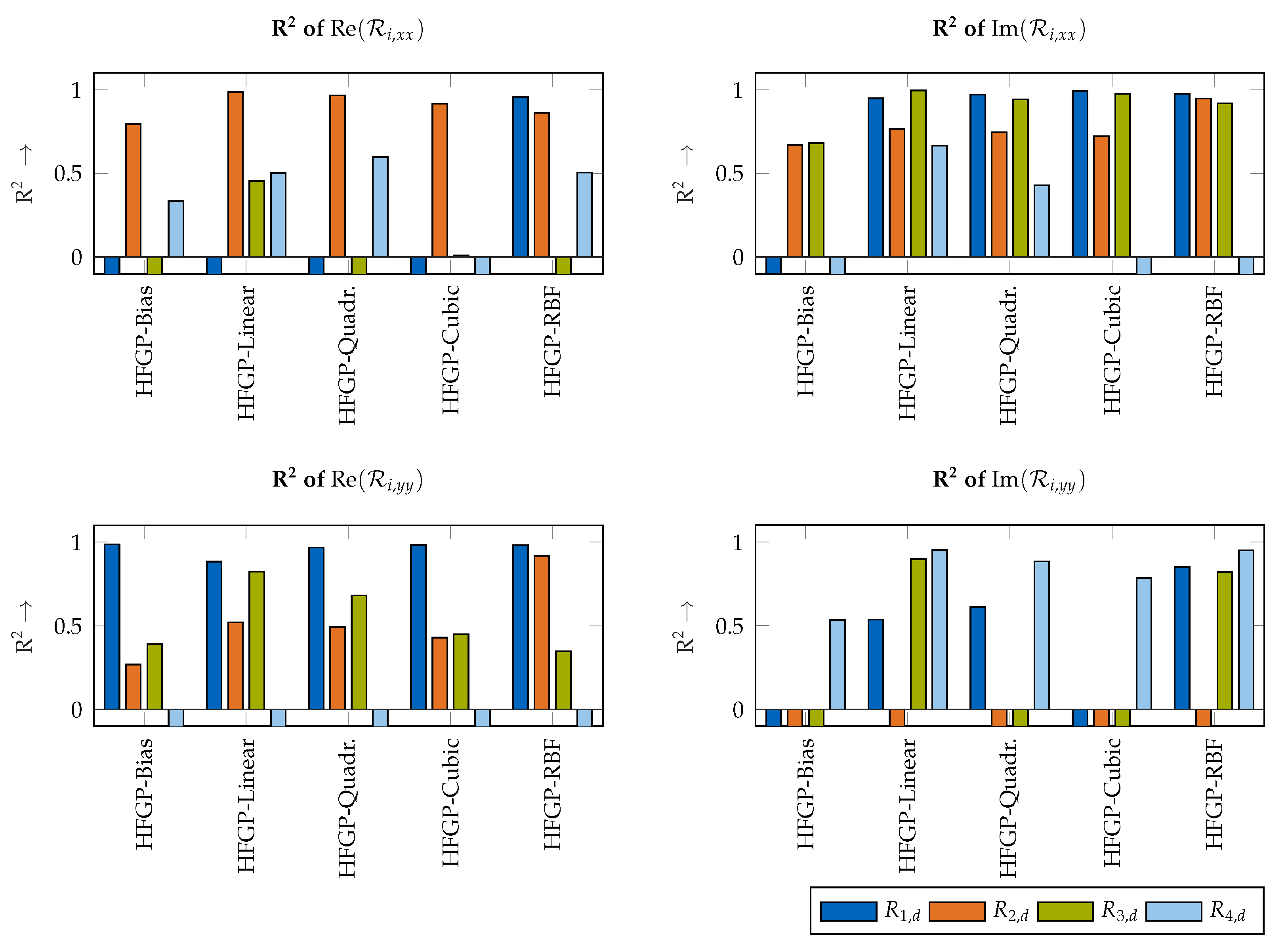
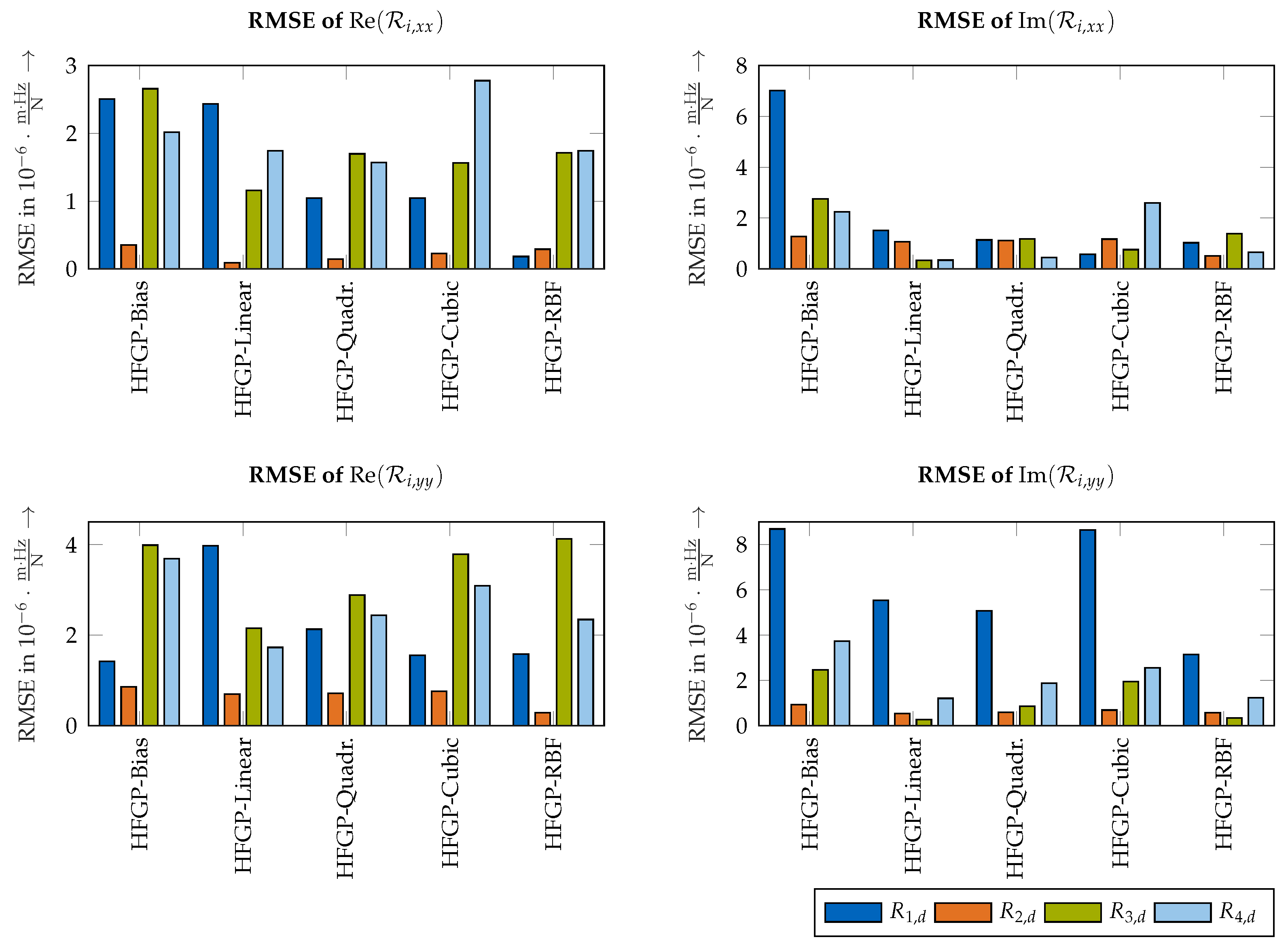
Analogously to the kernel selection process for the damping ratios, the five kernels (, , , and ) are benchmarked against each other to evaluate their performance in modeling the spatial behavior of the residues . As described in Section 2.3.3, each complex residue is modeled using two independent Gaussian processes, one for the real and one for the imaginary part. The resulting RMSEs for the real and imaginary parts of and are depicted in Figure 11. The resulting values for and are given in the Appendix E (see Figure A4).

Figure 11.
Benchmarks of different kernel designs for modeling spatial behavior of and .
The spatial behavior of the residues is best modeled using the RBF kernel, especially for the imaginary parts of the residues. It is assumed that the RBF kernel outperforms the other kernels, since its properties allow a more flexible approximation of the underlying system behavior and do not restrict the model behavior (unlike a linear kernel, for example). Hence, it is recommended to use an RBF kernel to model the spatial properties of the mode’s residues.
3.4. Reconstruction of Frequency Response Functions
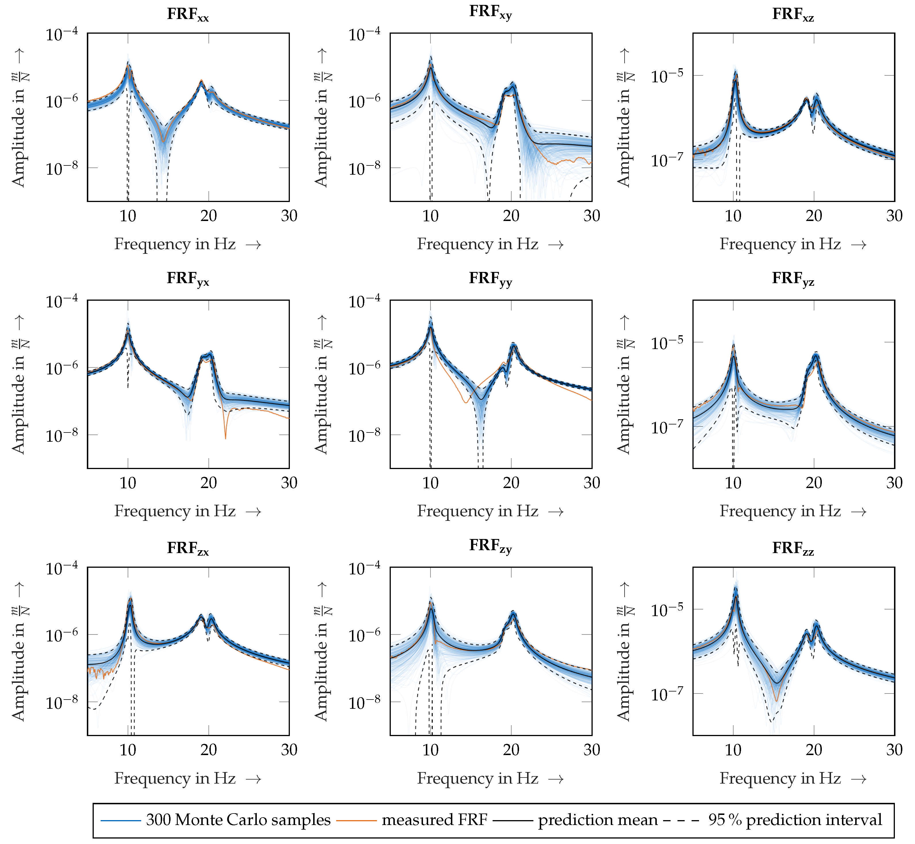
As presented in Section 2 and validated in Section 3.1, Section 3.2 and Section 3.3, the spatial properties of the robot dynamics, namely its natural frequencies, its damping ratios and its mode shapes, are modeled using probabilistic machine learning techniques. The strengths of the presented methodology can be illustrated using the reconstruction of the probabilistic frequency response function from the probabilistically modeled modal parameters (see Figure 12).
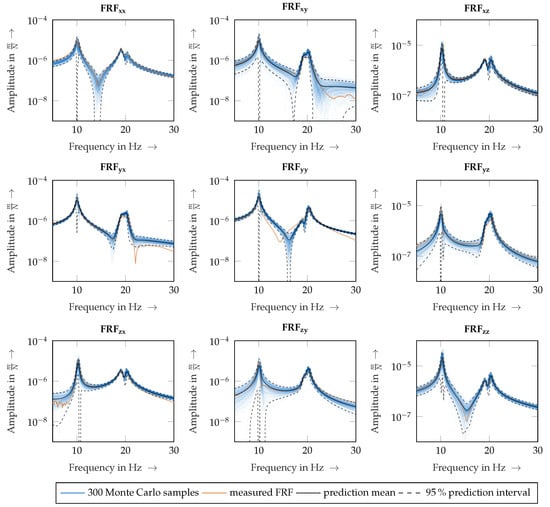
Figure 12.
Measured directional frequency response functions and model predictions at testing point using sampling strategy (for simplicity, only 300 of 10,000 Monte Carlo samples are illustrated).
To do so, a conventional quasi-Monte Carlo (QMC) algorithm was utilized to estimate the resulting uncertainty in the reconstructed frequency response functions based on the uncertainty in the model predictions for the modal parameters at . This point was not part of the training data. Detailed information on Monte Carlo and quasi-Monte Carlo techniques can be found in [27]. The random sampling during the QMC computation follow the Saltelli scheme (see [28] for detailed information).
The sampling strategy was chosen, so only five measurements in the workspace were taken into account during training (see Figure 5). During the Monte Carlo simulation, the directional frequency response functions were calculated times, based on random samples from the predicted probability distributions of , and . The modeling approach is able to take asymmetric frequency response behavior into account (e.g. ), as the directional residuals are trained independently of each other.
3.5. Implementation Details
All computations were performed in Matlab, Python, and C++. Table 1 summarizes the key software packages used. The model training computations and the QMC simulations were performed on a cloud server running with 10 cores (Intel(R) Xeon(R) Gold 6148 CPU @ 2.40 GHz) and 45 GB RAM under Ubuntu 18.04.

Table 1.
Used software packages.
4. Discussion
The validation results show that the proposed modeling approach makes it possible to model the spatial behavior of the robot dynamics in the form of its modal properties. Since probabilistic machine learning techniques are used, the model prediction does not only provide the estimated prediction mean, but also a reliable prediction uncertainty. The reconstructed frequency response functions are in good agreement with the measurements.
The performance evaluation indicates that the information fusion approach to modeling the spatial properties of the robot’s natural frequencies can significantly improve the model performance, in comparison with that of conventional Gaussian process regression techniques when only few measurements in the workspace are available. It is our intention to investigate optimal sampling techniques in the future: according to the human-in-the-loop-principle (also called Active Learning), an iterative algorithm should propose the optimal next measurement point within the workspace to reach satisfactory model performance with as few measurements as possible.
Furthermore, the presented methodology provides the fundamental methods needed to predict pose-dependant stability limits, for example by predicting pose-dependent stability lobes based on the pose-dependent robot dynamics. Such an application is particularly appealing if the model uncertainty is propagated to the stability prediction as well. Existing methods for propagating the uncertainty that arises during the cutting force coefficient identification can be extended by the presented modeling approach [33].
Hence, such a combined model can incorporate both the uncertainty of the robot’s structural dynamics as well as the uncertainty of the cutting force models.
The model is based on the estimated modal properties and not directly on the measured frequency response functions. However, state-of-the-art EMA methods still require domain expert knowledge (e.g., selecting an appropriate model order or selecting suitable poles) [34]. Hence, inaccuracies during the manual modal parameter extraction will result in inaccuracies in the trained models. It is advisable that further research is carried out in the field of automated and robust modal parameter estimation to model the robot’s dynamics as accurately as possible. This is especially important if the natural frequencies overlap. In this case, the distinction between the modes must be carried out carefully under consideration of the mode shapes. Such mode tracking algorithms can make use of the MAC criterion to quantify similarities of the mode shapes to track the spatial behavior within the workspace of the robot.
Additionally, the methodology was validated for measurement points in the horizontal x-y-plane with a constant TCP orientation, which allows the application for 2.5D machining operations in the horizontal plane. For more complex machining operations or applications in different heights, the workspace must be extended using measurement locations in the three-dimensional space or including data points which incorporate the robot’s kinematic redundancy (i.e., a rotation of the TCP around the tool’s rotation axis).
5. Conclusions
This paper presented a methodology for modeling the position-dependent dynamics of industrial robots. The methodology is based on data-driven methods for modeling the spatial behavior of the robot’s modal parameters.
The findings of the presented study are as follows:
- First, an information fusion approach to model the robot’s position-dependent natural frequencies improves the prediction accuracy significantly in comparison to that of conventional Gaussian process regression techniques, especially in scenarios with only a very small number of training data points. In those cases, the prediction uncertainty of conventional Gaussian processes is unreliable, whereas the uncertainty estimation of the linear information fusion scheme is reliable.
- Second, a detailed study was conducted to evaluate different kernel design choices for modeling the robot’s damping ratios and mode residues using conventional Gaussian process regression methods. The data analysis of the position-dependent damping ratios motivates the use of cubic kernels, whereas an RBF kernel is best suited for modeling the residues.
- Third, the position-dependent models can be used to estimate the position-dependent directional dynamics of the robot accurately and quantify the combined model uncertainty using a Monte Carlo algorithm.
Author Contributions
The authors contributed as follows to this publication: Conceptualization, M.B.; methodology, M.B.; software, M.B.; validation, M.B.; formal analysis, M.B.; investigation, M.B.; resources, M.F.Z.; data curation, M.B.; writing—original draft preparation, M.B.; writing—review and editing, M.B. and M.F.Z.; visualization, M.B.; supervision, M.F.Z.; project administration, M.F.Z.; funding acquisition, M.F.Z. All authors have read and agreed to the published version of the manuscript.
Funding
We express our gratitude to the Bavarian Ministry of Economic Affairs, Regional Development, and Energy for the funding of our research. The methodology will be extended in the research project “ProKIRo” (grant number DIK-2104-0057 DIK0367/01).
Institutional Review Board Statement
Not applicable.
Informed Consent Statement
Not applicable.
Conflicts of Interest
The authors declare that they have no conflict of interest.
Appendix A. Measurement Locations
Table A1.
Measurement locations (given in the robot’s base coordinate system).
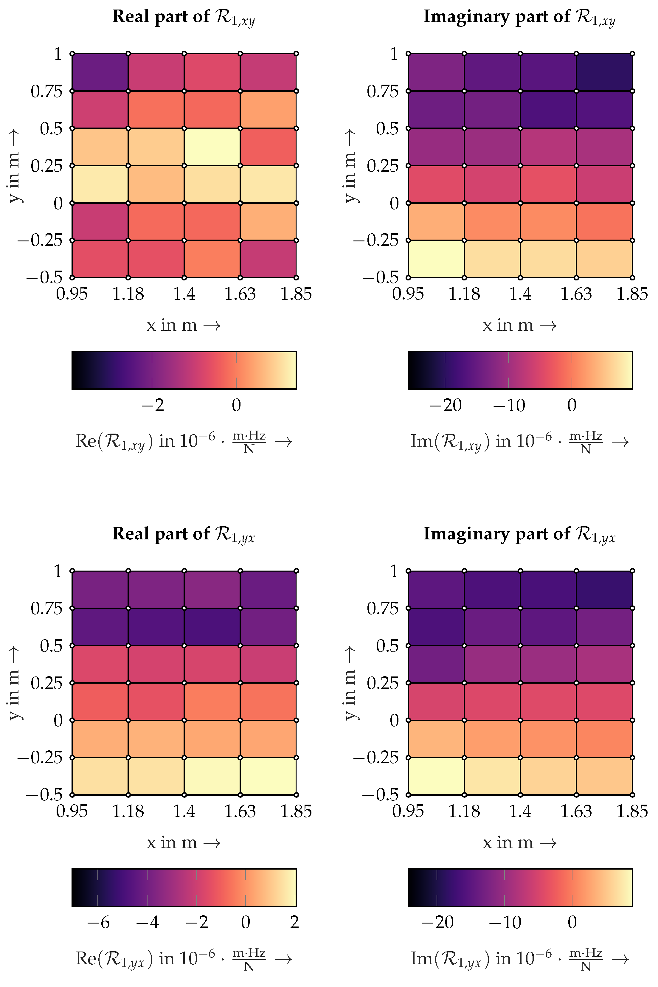
Appendix B. Cross Residuals Ri,xy and Ri,yx
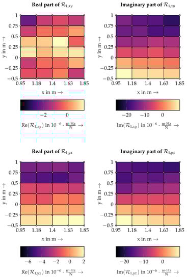
Figure A1.
Spatial behavior of cross residuals of first vibration mode.
Appendix C. Rigid Body Model of the Milling Robot
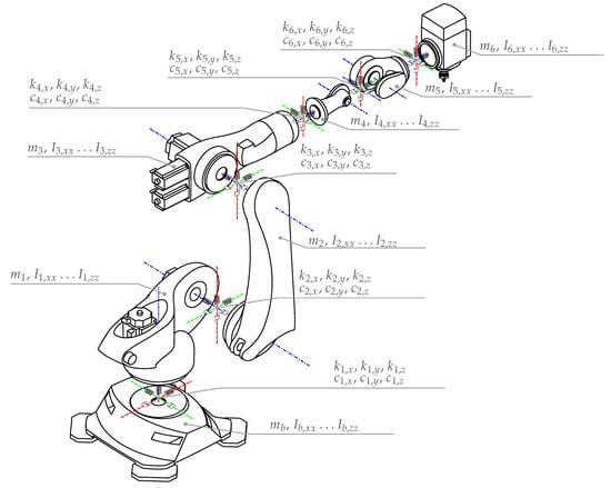
Figure A2.
Rigid body model of the robot. The orientation of the six local body coordinate systems are illustrated in colored lines (  = x,
= x,  = y,
= y,  = z.)
= z.)
= x, = y, = z.)
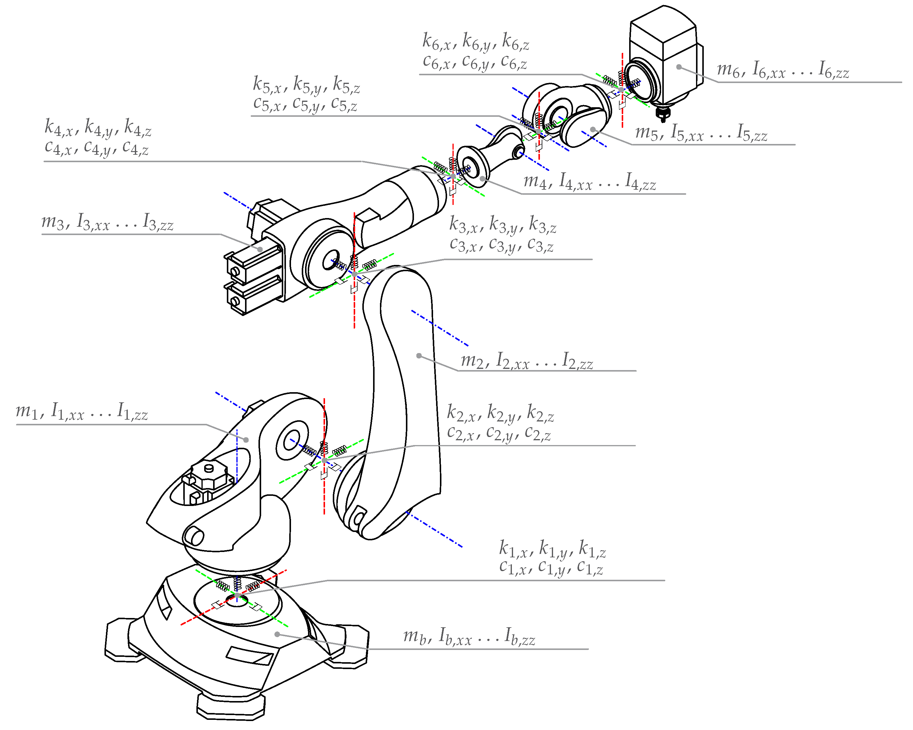
The mass, inertia and joint stiffness parameters (, and , respectively) of the robot model are as follows:
Appendix D. Mode Shape Visualization
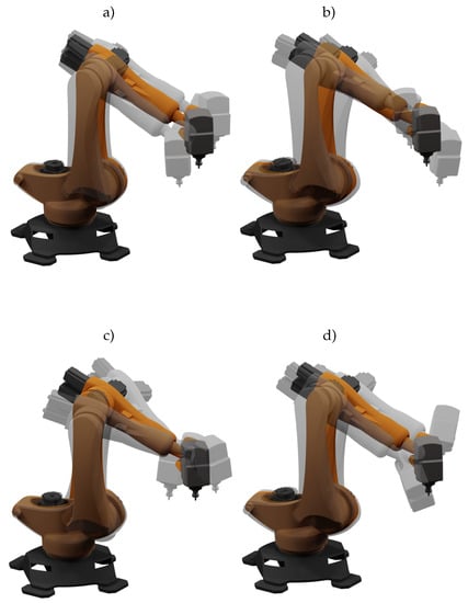
Figure A3.
The first four mode shapes (first mode 1 in a), second mode in b) third mode in c), fourth mode in d)), simulated with the rigid body model at .

Appendix E. R2 results of Ri,xx and Ri,yy
Figure A4.
Benchmarks of different kernel designs for modeling spatial behavior of and based on ( values lower than 0.1 are not displayed to their full extend for better comprehensibility).
References
- European Commission. The European Green Deal; European Commission: Brussels, Belgium, 2019. [Google Scholar]
- Baier, D.; Bachmann, A.; Zaeh, M.F. Towards wire and arc additive manufacturing of high-quality parts. Procedia CIRP 2020, 95, 54–59. [Google Scholar] [CrossRef]
- Fuchs, C.; Baier, D.; Semm, T.; Zaeh, M.F. Determining the machining allowance for WAAM parts. Prod. Eng. 2020, 14, 629–637. [Google Scholar] [CrossRef]
- Iglesias, I.; Sebastián, M.A.; Ares, J.E. Overview of the State of Robotic Machining: Current Situation and Future Potential. Procedia Eng. 2015, 132, 911–917. [Google Scholar] [CrossRef] [Green Version]
- Ji, W.; Wang, L. Industrial robotic machining: A review. Int. J. Adv. Manuf. Technol. 2019, 103, 1239–1255. [Google Scholar] [CrossRef] [Green Version]
- Karim, A.; Verl, A. Challenges and obstacles in robot-machining. In Proceedings of the 2013 44th International Symposium on Robotics, ISR 2013, Seoul, Korea, 24–26 October 2013. [Google Scholar]
- Rösch, O. Steigerung der Arbeitsgenauigkeit bei der Fräsbearbeitung Metallischer Werkstoffe mit Industrierobotern. Ph.D. Thesis, Technische Universität München, München, Germany, 2014. [Google Scholar]
- Zaeh, M.; Schnoes, F.; Obst, B.; Hartmann, D. Combined offline simulation and online adaptation approach for the accuracy improvement of milling robots. CIRP Ann. 2020, 69, 337–340. [Google Scholar] [CrossRef]
- Huynh, H.N.; Assadi, H.; Rivière-Lorphèvre, E.; Verlinden, O.; Ahmadi, K. Modelling the dynamics of industrial robots for milling operations. Robot.-Comput.-Integr. Manuf. 2020, 61, 101852. [Google Scholar] [CrossRef]
- Abele, E.; Rothenbücher, S.; Weigold, M. Cartesian compliance model for industrial robots using virtual joints. Prod. Eng. 2008, 2, 339–343. [Google Scholar] [CrossRef]
- Huynh, H.N.; Rivière-Lorphèvre, E.; Verlinden, O. Report of Robotic Machining Measurements Using a Stäubli TX200 Robot: Application to Milling. Volume 5B: 41st Mechanisms and Robotics Conference; American Society of Mechanical Engineers: New York, NY, USA, 2017; Volume 5B-2017. [Google Scholar]
- Dumas, C.; Caro, S.; Garnier, S.; Furet, B. Joint stiffness identification of six-revolute industrial serial robots. Robot.-Comput.-Integr. Manuf. 2011, 27, 881–888. [Google Scholar] [CrossRef] [Green Version]
- Busch, M.; Schnoes, F.; Elsharkawy, A.; Zaeh, M.F. Methodology for model-based uncertainty quantification of the vibrational properties of machining robots. Robot.-Comput.-Integr. Manuf. 2022, 73, 102243. [Google Scholar] [CrossRef]
- Nguyen, V.; Cvitanic, T.; Melkote, S. Data-Driven Modeling of the Modal Properties of a Six-Degrees-of-Freedom Industrial Robot and Its Application to Robotic Milling. J. Manuf. Sci. Eng. 2019, 141, 121006. [Google Scholar] [CrossRef]
- Nguyen, V.; Johnson, J.; Melkote, S. Active vibration suppression in robotic milling using optimal control. Int. J. Mach. Tools Manuf. 2020, 152, 103541. [Google Scholar] [CrossRef]
- Busch, M.; Schnoes, F.; Semm, T.; Zaeh, M.F.; Obst, B.; Hartmann, D. Probabilistic information fusion to model the pose-dependent dynamics of milling robots. Prod. Eng. 2020, 14, 435–444. [Google Scholar] [CrossRef]
- Peherstorfer, B.; Willcox, K.; Gunzburger, M. Survey of multifidelity methods in uncertainty propagation, inference, and optimization. arXiv 2018, arXiv:1806.10761. [Google Scholar] [CrossRef]
- Fernández-Godino, M.G.; Park, C.; Kim, N.H.; Haftka, R.T. Review of multifidelity models. arXiv 2016, arXiv:1609.07196. [Google Scholar]
- Liu, Y.P.; Altintas, Y. Predicting the position-dependent dynamics of machine tools using progressive network. Precis. Eng. 2022, 73, 409–422. [Google Scholar] [CrossRef]
- Verboven, P. Frequency-Domain System Identification for Modal Analysis. Ph.D. Thesis, Vrije Universiteit Brussel, Brussel, Belgium, 2002. [Google Scholar]
- Puzik, A. Genauigkeitssteigerung bei der Spanenden Bearbeitung mit Industrie- robotern durch Fehlerkompensation mit 3D-Piezo-Ausgleichsaktorik. Ph.D. Thesis, Universität Stuttgart, Stuttgart, Germany, 2011. [Google Scholar]
- Geradin, M.; Rixen, D.J. Mechanical Vibrations: Theory and Application to Structural Dynamics, 3rd ed.; John Wiley & Sons, Ltd.: Chichester, UK, 2015. [Google Scholar]
- Reinl, C.; Friedmann, M.; Bauer, J.; Pischan, M.; Abele, E.; Von Stryk, O. Model-based off-line compensation of path deviation for industrial robots in milling applications. In Proceedings of the IEEE/ASME International Conference on Advanced Intelligent Mechatronics, AIM, Budapest, Hungary, 3–7 July 2011; pp. 367–372. [Google Scholar]
- Kennedy, M.C.; O’Hagan, A. Predicting the output from a complex computer code when fast approximations are available. Biometrika 2000, 87, 1–13. [Google Scholar] [CrossRef] [Green Version]
- Perdikaris, P.; Raissi, M.; Damianou, A.; Lawrence, N.D.; Karniadakis, G.E. Nonlinear information fusion algorithms for robust multi-fidelity modeling. Proc. R. Soc. Math. Phys. Eng. Sci. 2016, 473, 751. [Google Scholar]
- Rasmussen, C.E.; Williams, C.K.I. Gaussian Processes for Machine Learning. Int. J. Neural Syst. 2006, 11, 3011–3015. [Google Scholar]
- Lemieux, C. Monte Carlo and Quasi-Monte Carlo Sampling; Springer Series in Statistics; Springer: New York, NY, USA, 2009. [Google Scholar] [CrossRef] [Green Version]
- Tennøe, S.; Halnes, G.; Einevoll, G.T. Uncertainpy: A Python Toolbox for Uncertainty Quantification and Sensitivity Analysis in Computational Neuroscience. Front. Neuroinform. 2018, 12, 1–29. [Google Scholar] [CrossRef] [PubMed] [Green Version]
- Zaletelj, K.; Bregar, T.; Gorjup, D.; Slavič, J. pyEMA. 2020. Available online: https://github.com/ladisk/pyEMA (accessed on 20 January 2022).
- Felis, M.L. RBDL: An efficient rigid-body dynamics library using recursive algorithms. Auton. Robot. 2017, 41, 495–511. [Google Scholar] [CrossRef]
- Sheffield Machine Learning Software. GPy: A Gaussian Process Framework in Python. 2012. Available online: http://github.com/SheffieldML/GPy (accessed on 20 January 2022).
- Paleyes, A.; Pullin, M.; Mahsereci, M.; Lawrence, N.; González, J. Emulation of physical processes with Emukit. In Proceedings of the Second Workshop on Machine Learning and the Physical Sciences, NeurIPS, Vancouver, BC, Canada, 8–14 December 2019. [Google Scholar]
- Busch, M.; Schmucker, B.; Zaeh, M.F. Rapid uncertainty quantification of the stability analysis using a probabilistic estimation of the process force parameters. MM Sci. J. 2021, 2021, 4978–4983. [Google Scholar] [CrossRef]
- Lau, J.; Lanslots, J.; Peeters, B.; Van Der Auweraer, H. Automatic modal analysis: Reality or myth? In Proceedings of the IMAC 25, Orlando, FL, USA, 19–22 February 2007. [Google Scholar]


Publisher’s Note: MDPI stays neutral with regard to jurisdictional claims in published maps and institutional affiliations. |
© 2022 by the authors. Licensee MDPI, Basel, Switzerland. This article is an open access article distributed under the terms and conditions of the Creative Commons Attribution (CC BY) license (https://creativecommons.org/licenses/by/4.0/).