Abstract
E-type -attractor models of single-field inflation were generalized further in order to accommodate production of primordial black holes (PBHs) via adding a near-inflection point to the inflaton scalar potential at smaller scales, in good agreement with measurements of cosmic microwave background (CMB) radiation. A minimal number of new parameters were used but their fine-tuning was maximized in order to increase the possible masses of PBHs formed during an ultra-slow-roll phase, leading to a large enhancement in the power spectrum of scalar (curvature) perturbations by 6 or 7 orders of magnitude against the power spectrum of perturbations observed in CMB. It was found that extreme fine-tuning of the parameters in our models can lead to the formation of moon-sized PBHs, with masses of up to g, still in agreement with CMB observations. Quantum corrections are known to lead to the perturbative upper bound on the amplitude of large scalar perturbations responsible for PBH production. The quantum (one-loop) corrections in our models were found to be suppressed by one order of magnitude for PBHs with masses of approximately g, which may form the whole dark matter in the Universe.
1. Introduction
The paradigm of cosmological inflation proposed by Guth and Linde [1,2] is a possible answer to internal problems of standard (Einstein–Friedmann) cosmology. Inflation as the amplifier of curvature perturbations is also a possible origin of seeds of structure formation in the early Universe [3,4]. The existence of inflation is supported by measurements of cosmic microwave background (CMB) radiation [5,6,7].
The CMB measurements highlight a small window into high energy physics in the form of the power spectrum of perturbations on limited (CMB) scales and lead to important restrictions on viable inflationary models, but do not allow a reconstruction of the unique underlying inflationary model. There are uncertainties even among the simplest single-field (quintessence) models of inflation in the form of the (canonical) inflaton scalar potential. These uncertainties can be exploited to win more room for the single-field inflationary models by extending the flexibility of their predictions about inflation, while simultaneously describing the formation of primordial black holes (PBHs) from large scalar perturbations at lower (than CMB) scales [8,9]. A standard mechanism of PBH formation is given by adding a near-inflection point to the inflaton potential [10,11,12,13]. The observational constraints on PBHs are also subject to uncertainties [14,15] even in the limited context of the single-field models of inflatons with a near-inflection point [16]. Therefore, it makes sense to investigate the amount of flexibility of fine-tuning in the well-motivated models of inflation and PBH production on a case-by-case basis.
In this paper, we revisit the -attractor (single-field) inflationary models introduced in refs. [17,18] and propose new generalizations of them. The simplest attractor model with is given by the famous Starobinsky model [19] motivated by gravitational interactions, with an inflaton as the Nambu–Goldstone boson associated with the spontaneous breaking of scale invariance [20]. After taking into account the CMB constraints alone, the Starobinsky model has no free parameters and leads to a sharp prediction for the tensor power spectrum tilt of the gravitational waves induced by inflation. The (canonical) inflaton scalar potential in the Starobinsky model reads
where is the inflaton mass and is the reduced Planck mass. This leads to the Mukhanov–Chibisov formula [21] for the tilt of scalar perturbations, , and the tensor-to-scalar ratio , where is the number of e-folds measuring the duration of inflation, in very good agreement with the CMB measurements [5,6,7],
for . Actually, only the leading exponent in Equation (1), i.e., the term linear in y, is relevant for the tilts during slow-roll inflation predicted by the Starobinsky model. This simple observation allows one to extend the Starobinsky model by a single new parameter entering the new variable y as [17,18]
without changing the Mukhanov–Chibisov formula for ns. However, the tensor-to-scalar ratio changes via
thus adding more flexibility against future measurements of r.
The scalar potentials of the simplest -attractor models fall into two classes: the simplest E-models have the scalar potential shown in Equation (1) but with the variable y defined by Equation (3), whereas the simplest T-models have the scalar potential
where the scale of inflation is given by . Further generalizations are also possible, while keeping the predictions for the cosmological tilts and r during inflation. For example, generalized T-models with the scalar potential and a monotonically increasing (during slow roll) function were used in refs. [22,23,24] for engineering a near-inflection point in the potential and PBH production, see also ref. [25]. The T-model potentials can also be made periodic by changing their global shape after replacing the function in Equation (5) by the periodic (Jacobi) elliptic function with the elliptic modulus , in the limit
thus combining theoretically attractive features of chaotic inflation and natural inflation.
The power spectrum of scalar perturbations in some generalized T-models with a near-inflection point for PBH production and the related spectrum of induced gravitational waves were derived in ref. [26]. Similar results for the E-models were obtained in ref. [27].
The scalar potential used in ref. [27] has the form
with y defined by Equation (3) and the new (positive) parameters and needed for engineering a near-inflection point. The ansatz (7) was motivated in ref. [26] by small values of y during slow-roll inflation, keeping agreement with CMB measurements [28] and having a near-inflection point at lower scales for certain (fine-tuned) values of the new parameters, which was needed for viable inflation and PBH production.1
As was demonstrated in ref. [27], the potential (7) leads to PBH production, with the PBH masses corresponding to asteroid-sized black holes in the small mass window, where those PBHs may form the whole dark matter in the Universe. However, in ref. [27], it was achieved at the price of having the agreement with the CMB value of outside (though within ), with fine tuning the parameters and ignoring quantum corrections. Actually, the higher the masses of the PBH produced, the lower (in red) the scalar tilt becomes. Therefore, the following questions arise:
- Is it possible to reach the perfect (within ) agreement with the CMB value of in E-type models of inflation and PBH formation?
- Is it possible to increase the PBH masses beyond asteroid size?
- Is it possible so suppress (one-loop) quantum corrections?
In this communication, we improve our earlier findings about E-models in order to achieve a perfect agreement (inside ) with the observed values of CMB tilts, reconsider PBH formation and comment on (one-loop) quantum corrections in our new E-type models.
2. More General E-Models
At least two extra parameters are needed, as in Equation (7), for engineering a near-inflection point. However, the parameters in Equation (7) do not have clear meaning, so it is useful to replace them by other (related) parameters as [23,27]
The two real parameters have a clear meaning; when , the potential has an inflection point at only and when , the potential also has a local minimum (dip) and a local maximum (bump) at , respectively, while both extrema are equally separated from the inflection point,
The analyticity of the inflaton potential with respect to y (near ), responsible for the infinite plateau at , can be relaxed by adding negative powers of y. This is motivated by supergravity cosmology [30] and string cosmology [31], where such terms naturally appear. For our purposes, we use this resource in the minimalistic manner by adding merely a single term with a negative power to the E-model potential (7). We find adding a term proportional to is more efficient than , so we only consider the case of
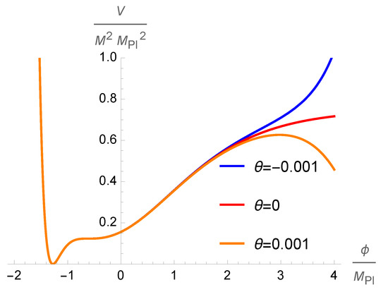
with the new (third) real parameter that is supposed to be small enough in order to keep agreement with CMB. An impact of the new parameter on the shape of the scalar potential is illustrated on Figure 1. The shape needed for inflation and PBH production is not generic, and is found after scanning the parameter space and fine-tuning the parameter values.

Figure 1.
The potential (10) with , and for the selected values of .
As is clear from Figure 1 that a negative brings the potential up, and a positive brings the potential down, against the plateau for for large values of .
The impact of the new parameter on the slow-roll (SR) parameters
is displayed in Figure 2, which shows that the SR phase is in agreement with CMB. The end of this SR phase of inflation is determined by the condition . The standard pivot scale of the horizon exit, when scalar perturbations leave the horizon, is .

Figure 2.
The -dependence of the slow-roll parameters at , and for the selected values of .
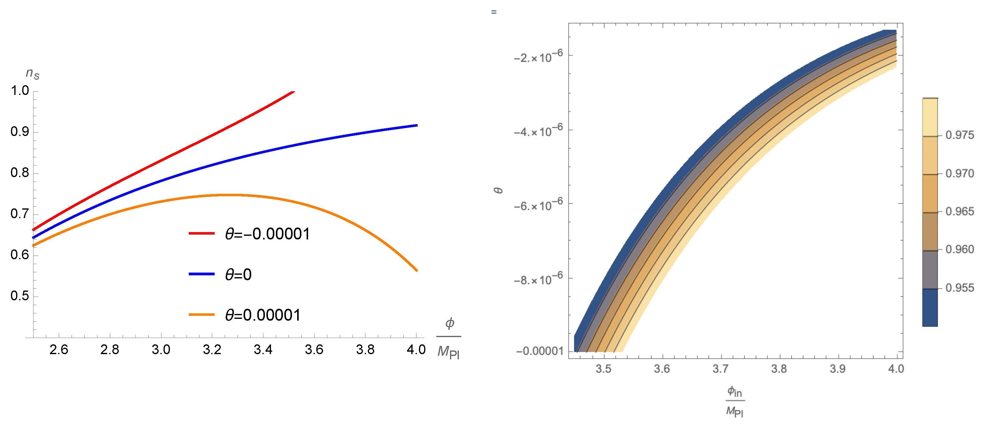
The raising tail of the profile of near the horizon exit on the left plot in Figure 2 increases the tensor-to-scalar ratio r, while the need to increase implies the negative sign of , as is clear from the right plot in Figure 2. To increase the PBH masses (see the next section), we can go up to the maximal value of according to Equation (2).
Our numerical solutions of the standard equations of motion for the inflaton as a function of time t and the Hubble function with the same values of the parameters for the selected values of are shown in Figure 3. It shows the duration of inflation, defined by the length of the plateau, for different values of .

Figure 3.
The time evolution of the inflaton and the Hubble function (where is the cosmic factor in the metric of a spatially flat Friedmann universe) with the parameters , and , and the horizon exit at .
The Hubble flow functions are defined by
The (numerically derived) dynamics of these function are shown in Figure 4.

Figure 4.
The Hubble flow functions and with the parameters , and .
Figure 4 shows the existence of the ultra-slow-roll (USR) phase [13,32], where the first derivative of the inflaton potential and the Hubble flow function drop to very low values. During the USR phase, the Hubble flow function also drops from near zero to
Our findings for the CMB scalar tilt with the fine-tuned parameters are displayed in Figure 5, where we also show the dependence of upon and .

Figure 5.
The dependence of the CMB scalar tilt upon the inflaton field (on the left) and and at the horizon exit (on the right). The other parameters are , and .
With the exit value of and the parameter , we find
which are fully consistent with the CMB measurements (2). This value of r saturates the current CMB upper bound on the tensor-to-scalar ratio and maximizes the PBH masses (see the next section).
3. Power Spectrum and PBH Formation
A standard procedure of (numerically) computing the power spectrum of scalar (curvature) perturbations depending upon scale k is based on the Mukhanov–Sasaki (MS) equation [33,34]. There is a simple analytic formula for in the SR approximation, see, e.g., ref. [12], which reads
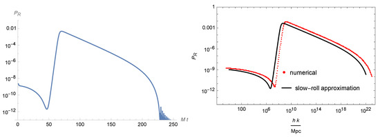
We used both approaches in our models and found that the difference between the exact results from numerically solving the MS equation and those derived from the SR Formula (15) is small (see Figure 6 as an example), and is irrelevant for our purposes.

Figure 6.
The power spectrum of scalar perturbations with the parameters , , , and . The peak location is at Mpc.
Knowing the location of the peak in the power spectrum allows us to estimate the masses of the produced PBH as [14,15]
where is the mass of the sun, . For instance, with the peak value Mpc, we obtain
which is just between the mass of the moon, g, and the mass of the Earth, g. The PBH mass (17) should be understood as the maximal PBH mass possible in our classical E-models after extreme fine-tuning of the parameters, in agreement with CMB measurements.
In regard to other possible values of the CMB tilts and r, the squared amplitude of curvature perturbations at the horizon exit , and the related PBH masses according to Equation (16), derived from our models, are summarized in Table 1.

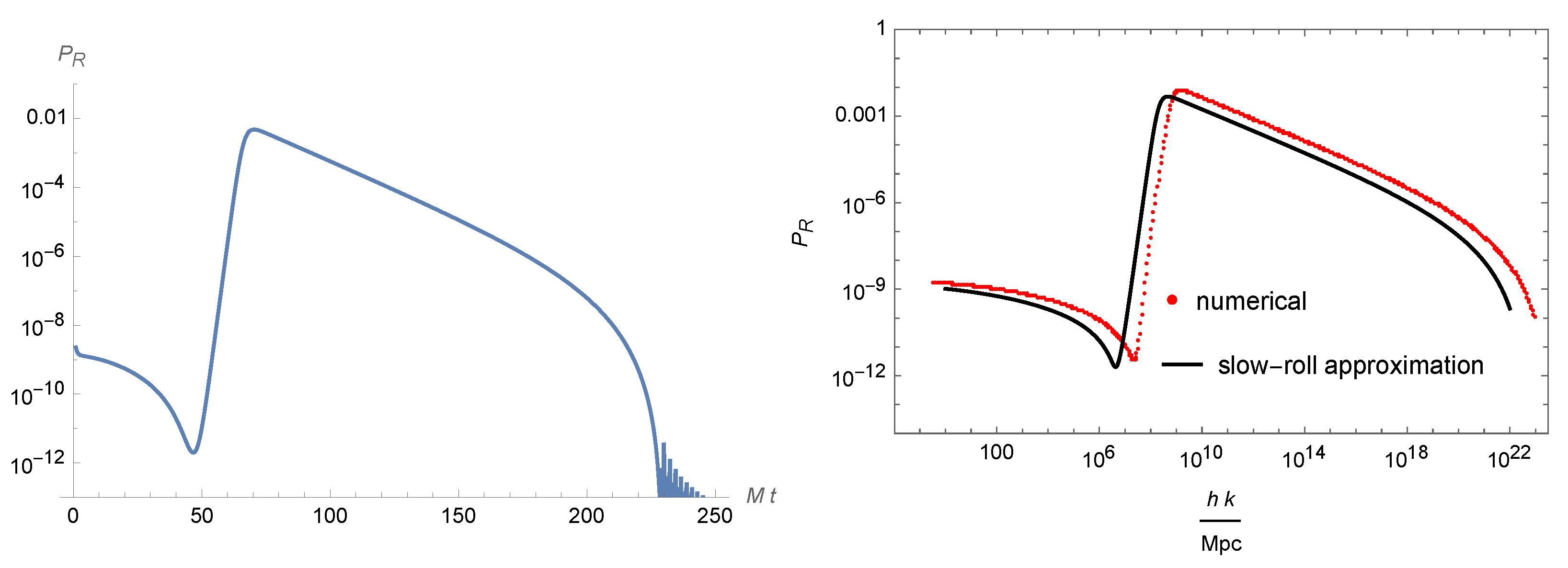
The plots of the Hubble flow functions (12) in the particular model with the parameters , , and are given in Figure 7. Figure 7 shows the existence of a USR phase with between two SR phases, where the USR begins at and ends at with the USR duration of . Our plots in Figure 7 are similar to those in the literature for the inflationary models with a USR phase, see, e.g., Figure 1 in ref. [35] for comparison.

Figure 7.
The Hubble flow functions (12) for the parameters , , and . The other related values are , Mpc, Mpc and . Both plots show the USR phase for . The plot (right) is the superposition of the Hubble flows for and .
At the end of this section, we briefly comment on expected one-loop quantum corrections in our E-models by using the results and discussions in refs. [36,37,38,39,40,41].
The Hubble flow function can be approximated by a step function during the USR phase, which leads to the (one-loop) perturbative bound on validity of the classical results in the form [36,38]
where the amplitude squared of scalar curvature perturbations was taken from refs. [36,38] and is of the order . Given , Equation (18) implies the perturbative bound on the power spectrum as [36,38]
which might rule out classical results about PBH production in any single-field model of inflation with a near-inflection point. In our models, we have the smooth function and that implies a stronger bound,
However, the values of given in Table 1 are smaller (though not much smaller) than the bound (20). There is an uncertainty in the value of used in refs. [36,38] for PBH production, which is related to an uncertainty in the smoothed density contrast constant and relaxes the peak value (needed for PBH formation) to [39]. Therefore, our classical results obtained in the fine-tuned E-models for PBH production are still not ruled out by quantum corrections, at least in regard to the bottom line in Table 1.
4. Conclusions
Production of PBHs with masses beyond the Hawking (black hole) radiation limit of g in the early Universe is not a generic feature of single-field models of inflation with a near-inflection point because it requires fine-tuning of the parameters defining the inflaton potential and depends upon the duration of the SR and USR phases. We adopted maximal fine-tuning with the minimal number of parameters in the (generalized) E-type -attractor models of inflation, while keeping agreement with CMB measurements.
We numerically scanned the parameter space of our models in order to find the parameter values leading to a significant enhancement (by to times) in the power spectrum of scalar (curvature) perturbations. We confirmed the high sensitivity of our results with a choice of the parameters, in agreement with general expectations [42].
Compared to ref. [27], we added the new parameter in the new term (proportional to ) in the inflaton scalar potential in order to reach perfect agreement with the observed CMB values of the cosmological tilts and r.
Fine-tuning of the parameters in our models was needed not only to match the CMB measurements (inflation is robust in the E-models) but also to generate PBH production at lower scales during the USR phase, which would lead to a sizable portion of PBHs in the current dark matter. The equations for PBH mass in the literature [14,15,16] are sensitive to a detailed shape of the peak in the power spectrum and the USR phase duration, so in this paper, we only used the rough estimate in Equation (16). Taking into account these uncertainties may change the PBH masses by 1–2 orders of magnitude.
Though production of PBHs with masses of approximately g was found to be possible in classical theory (see the first row in Table 1), those PBHs may be ruled out by quantum corrections. In regard to the asteroid-sized PBHs with masses of approximately g, which are possible candidates for the whole dark matter in the Universe [14,15,27], the quantum (one-loop) corrections were shown to be suppressed by one order of magnitude according to the estimate in Equation (20) and the third row of Table 1. Hence, our generalized E-models of inflation and PBH production are still not ruled out.
Author Contributions
All authors contributed equally. All authors have read and agreed to the published version of the manuscript.
Funding
This research was partially supported by Tomsk State University under the development program Priority-2030. SVK was also supported by Tokyo Metropolitan University, the Japanese Society for Promotion of Science under grant no. 22K03624 and the World Premier International Research Center Initiative, MEXT, Japan.
Data Availability Statement
No new data was created.
Conflicts of Interest
The authors declare no conflict of interest.
Note
| 1 | Similar models were proposed and studied in ref. [29]. |
References
- Guth, A.H. The Inflationary Universe: A Possible Solution to the Horizon and Flatness Problems. Phys. Rev. D 1981, 23, 347–356. [Google Scholar] [CrossRef]
- Linde, A.D. A New Inflationary Universe Scenario: A Possible Solution of the Horizon, Flatness, Homogeneity, Isotropy and Primordial Monopole Problems. Phys. Lett. B 1982, 108, 389–393. [Google Scholar] [CrossRef]
- Mukhanov, V. Physical Foundations of Cosmology; Cambridge University Press: Oxford, UK, 2005. [Google Scholar] [CrossRef]
- Liddle, A.R.; Lyth, D.H. Cosmological Inflation and Large Scale Structure; Cambridge University Press: Cambridge, UK, 2000. [Google Scholar]
- Akrami, Y. et al. [Planck Collaboration] Planck 2018 results. X. Constraints on inflation. Astron. Astrophys. 2020, 641, A10. [Google Scholar] [CrossRef]
- Ade, P.A.R. et al. [BICEP, Keck Collaboration] Improved Constraints on Primordial Gravitational Waves using Planck, WMAP, and BICEP/Keck Observations through the 2018 Observing Season. Phys. Rev. Lett. 2021, 127, 151301. [Google Scholar] [CrossRef]
- Tristram, M.; Tristram, M.; Banday, J.; Górski, M.; Keskitalo, R.; Lawrence, R.; Andersen, J.; Barreiro, B.; Borrill, J.; Colombo, L.; et al. Improved limits on the tensor-to-scalar ratio using BICEP and Planck data. Phys. Rev. D 2022, 105, 083524. [Google Scholar] [CrossRef]
- Novikov, I.; Zeldovic, Y. Cosmology. Ann. Rev. Astron. Astrophys. 1967, 5, 627–649. [Google Scholar] [CrossRef]
- Hawking, S. Gravitationally collapsed objects of very low mass. Mon. Not. R. Astron. Soc. 1971, 152, 75. [Google Scholar] [CrossRef]
- Ivanov, P.; Naselsky, P.; Novikov, I. Inflation and primordial black holes as dark matter. Phys. Rev. D 1994, 50, 7173–7178. [Google Scholar] [CrossRef] [PubMed]
- Garcia-Bellido, J.; Linde, A.D.; Wands, D. Density perturbations and black hole formation in hybrid inflation. Phys. Rev. D 1996, 54, 6040–6058. [Google Scholar] [CrossRef] [PubMed]
- Garcia-Bellido, J.; Ruiz Morales, E. Primordial black holes from single field models of inflation. Phys. Dark Univ. 2017, 18, 47–54. [Google Scholar] [CrossRef]
- Germani, C.; Prokopec, T. On primordial black holes from an inflection point. Phys. Dark Univ. 2017, 18, 6–10. [Google Scholar] [CrossRef]
- Carr, B.; Kohri, K.; Sendouda, Y.; Yokoyama, J. Constraints on primordial black holes. Rep. Prog. Phys. 2021, 84, 116902. [Google Scholar] [CrossRef] [PubMed]
- Escrivà, A.; Kuhnel, F.; Tada, Y. Primordial Black Holes. arXiv 2022, arXiv:2211.05767. [Google Scholar]
- Karam, A.; Koivunen, N.; Tomberg, E.; Vaskonen, V.; Veermäe, H. Anatomy of single-field inflationary models for primordial black holes. arXiv 2023, arXiv:2205.13540. [Google Scholar] [CrossRef]
- Kallosh, R.; Linde, A. Universality Class in Conformal Inflation. J. Cosmol. Astropart. Phys. 2013, 7, 002. [Google Scholar] [CrossRef]
- Galante, M.; Kallosh, R.; Linde, A.; Roest, D. Unity of Cosmological Inflation Attractors. Phys. Rev. Lett. 2015, 114, 141302. [Google Scholar] [CrossRef] [PubMed]
- Starobinsky, A.A. A new type of isotropic cosmological models without singularity. Phys. Lett. B 1980, 91, 99–102. [Google Scholar] [CrossRef]
- Ketov, S.V.; Starobinsky, A.A. Inflation and non-minimal scalar-curvature coupling in gravity and supergravity. J. Cosmol. Astropart. Phys. 2012, 8, 22. [Google Scholar] [CrossRef]
- Mukhanov, V.F.; Chibisov, G.V. Quantum Fluctuations and a Nonsingular Universe. JETP Lett. 1981, 33, 532–535. [Google Scholar]
- Dalianis, I.; Kehagias, A.; Tringas, G. Primordial black holes from α-attractors. J. Cosmol. Astropart. Phys. 2019, 1, 037. [Google Scholar] [CrossRef]
- Iacconi, L.; Assadullahi, H.; Fasiello, M.; Wands, D. Revisiting small-scale fluctuations in α-attractor models of inflation. J. Cosmol. Astropart. Phys. 2022, 6, 7. [Google Scholar] [CrossRef]
- Braglia, M.; Linde, A.; Kallosh, R.; Finelli, F. Hybrid α-attractors, primordial black holes and gravitational wave backgrounds. J. Cosmol. Astropart. Phys. 2023, 2023, 033. [Google Scholar] [CrossRef]
- Frolovsky, D.; Ketov, S.V. Fitting power spectrum of scalar perturbations for primordial black hole production during inflation. Astronomy 2023, 2, 47–57. [Google Scholar] [CrossRef]
- Frolovsky, D.; Ketov, S.V.; Saburov, S. Formation of primordial black holes after Starobinsky inflation. Mod. Phys. Lett. A 2022, 37, 2250135. [Google Scholar] [CrossRef]
- Frolovsky, D.; Ketov, S.V.; Saburov, S. E-models of inflation and primordial black holes. Front. Phys. 2022, 10, 1005333. [Google Scholar] [CrossRef]
- Ivanov, V.R.; Ketov, S.V.; Pozdeeva, E.O.; Vernov, S.Y. Analytic extensions of Starobinsky model of inflation. J. Cosmol. Astropart. Phys. 2022, 3, 058. [Google Scholar] [CrossRef]
- Mishra, S.S.; Sahni, V. Primordial Black Holes from a tiny bump/dip in the Inflaton potential. J. Cosmol. Astropart. Phys. 2020, 4, 007. [Google Scholar] [CrossRef]
- Aldabergenov, Y.; Ketov, S.V. Primordial black holes from Volkov-Akulov-Starobinsky supergravity. Fortsch. Phys. 2023, 2023, 2300039. [Google Scholar] [CrossRef]
- Cicoli, M.; Conlon, J.P.; Maharana, A.; Parameswaran, S.; Quevedo, F.; Zavala, I. String Cosmology: From the Early Universe to Today. arXiv 2023, arXiv:2303.04819. [Google Scholar]
- Dimopoulos, K. Ultra slow-roll inflation demystified. Phys. Lett. B 2017, 775, 262–265. [Google Scholar] [CrossRef]
- Mukhanov, V.F. Gravitational Instability of the Universe Filled with a Scalar Field. JETP Lett. 1985, 41, 493–496. [Google Scholar]
- Sasaki, M. Large Scale Quantum Fluctuations in the Inflationary Universe. Prog. Theor. Phys. 1986, 76, 1036. [Google Scholar] [CrossRef]
- Liu, J.; Guo, Z.-K.; Cai, R.-G. Analytical approximation of the scalar spectrum in the ultraslow-roll inflationary models. Phys. Rev. D 2020, 101, 083535. [Google Scholar] [CrossRef]
- Kristiano, J.; Yokoyama, J. Ruling Out Primordial Black Hole Formation from Single-Field Inflation. arXiv 2022, arXiv:2211.03395. [Google Scholar]
- Riotto, A. The Primordial Black Hole Formation from Single-Field Inflation is Not Ruled Out. arXiv 2023, arXiv:2301.00599. [Google Scholar]
- Kristiano, J.; Yokoyama, J. Response to criticism on “Ruling Out Primordial Black Hole Formation From Single-Field Inflation”: A note on bispectrum and one-loop correction in single-field inflation with primordial black hole formation. arXiv 2023, arXiv:2303.00341. [Google Scholar]
- Riotto, A. The Primordial Black Hole Formation from Single-Field Inflation is Still Not Ruled Out. arXiv 2023, arXiv:2303.01727. [Google Scholar]
- Choudhury, S.; Panda, S.; Sami, M. Quantum loop effects on the power spectrum and constraints on primordial black holes. arXiv 2023, arXiv:2303.06066. [Google Scholar]
- Firouzjahi, H.; Riotto, A. Primordial Black Holes and Loops in Single-Field Inflation. arXiv 2023, arXiv:2304.07801. [Google Scholar]
- Cole, P.S.; Gow, A.D.; Byrnes, C.T.; Patil, S.P. Primordial black holes from single-field inflation: A fine-tuning audit. arXiv 2023, arXiv:2304.01997. [Google Scholar]
Disclaimer/Publisher’s Note: The statements, opinions and data contained in all publications are solely those of the individual author(s) and contributor(s) and not of MDPI and/or the editor(s). MDPI and/or the editor(s) disclaim responsibility for any injury to people or property resulting from any ideas, methods, instructions or products referred to in the content. |
© 2023 by the authors. Licensee MDPI, Basel, Switzerland. This article is an open access article distributed under the terms and conditions of the Creative Commons Attribution (CC BY) license (https://creativecommons.org/licenses/by/4.0/).


