Feature-Based Classification Neural Network for Kepler Light Curves from Quarter 1


Abstract
:1. Introduction
2. Data
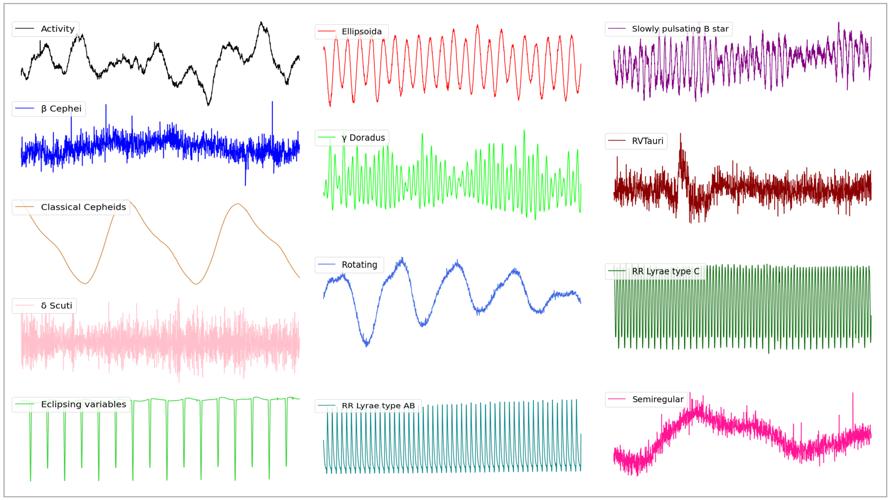
2.1. Data Set
2.2. Feature Extraction
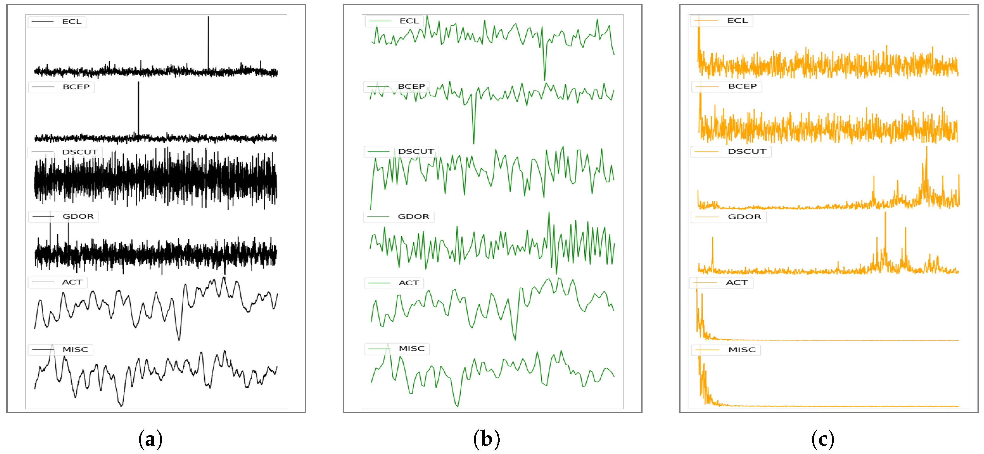
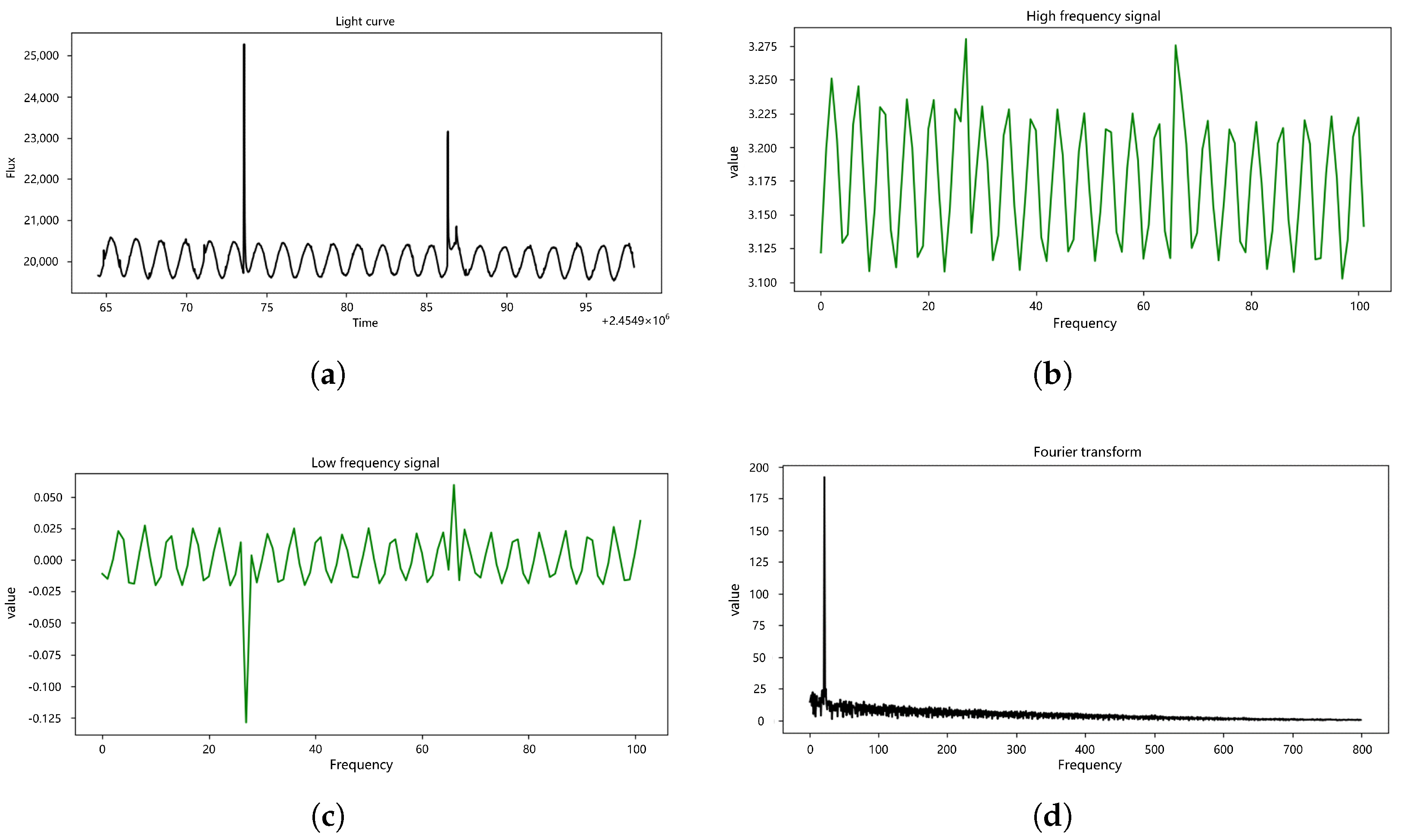
2.2.1. Frequency Domain Attributes
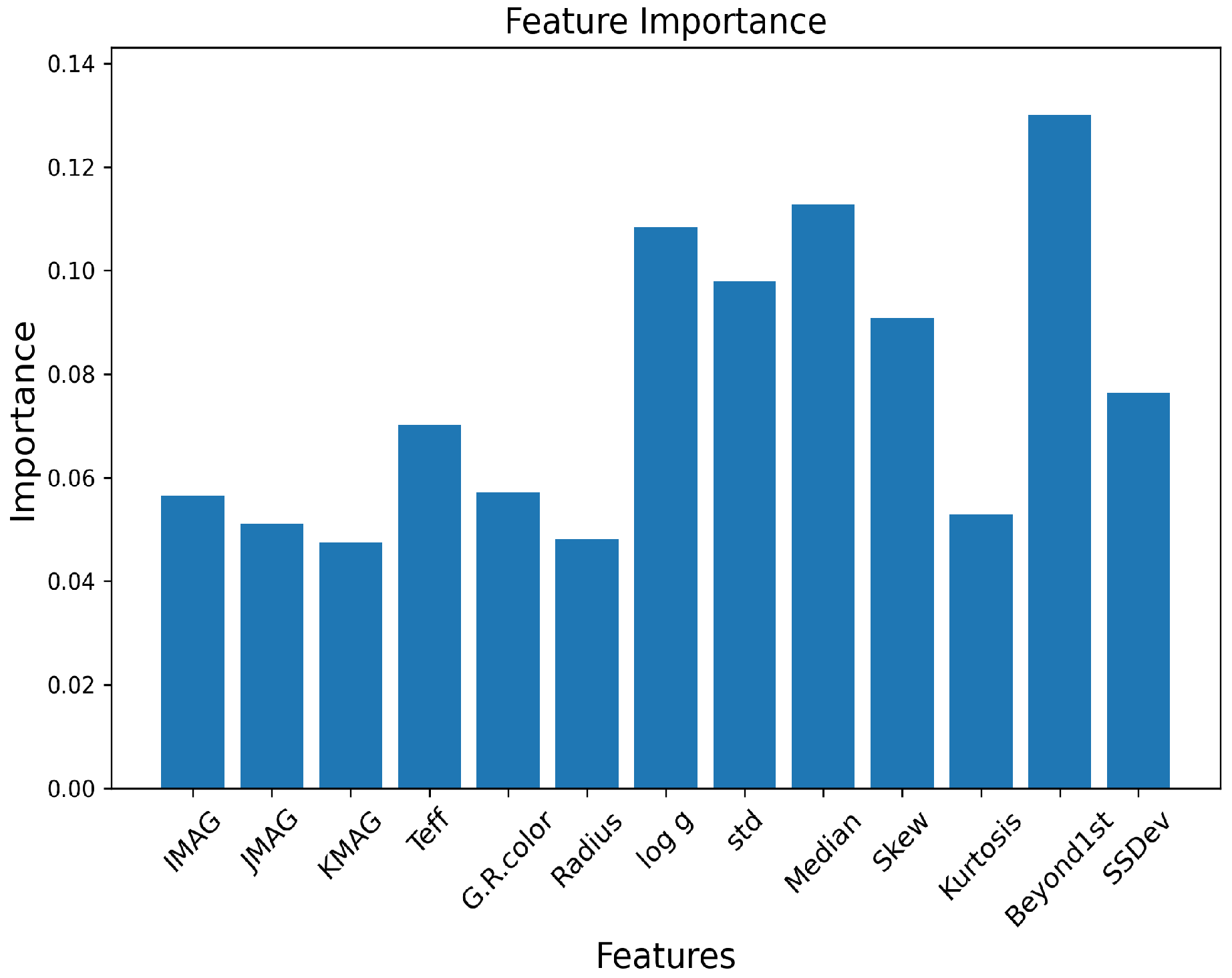
2.2.2. Other Attributes
2.3. Dimension of Features
3. Models
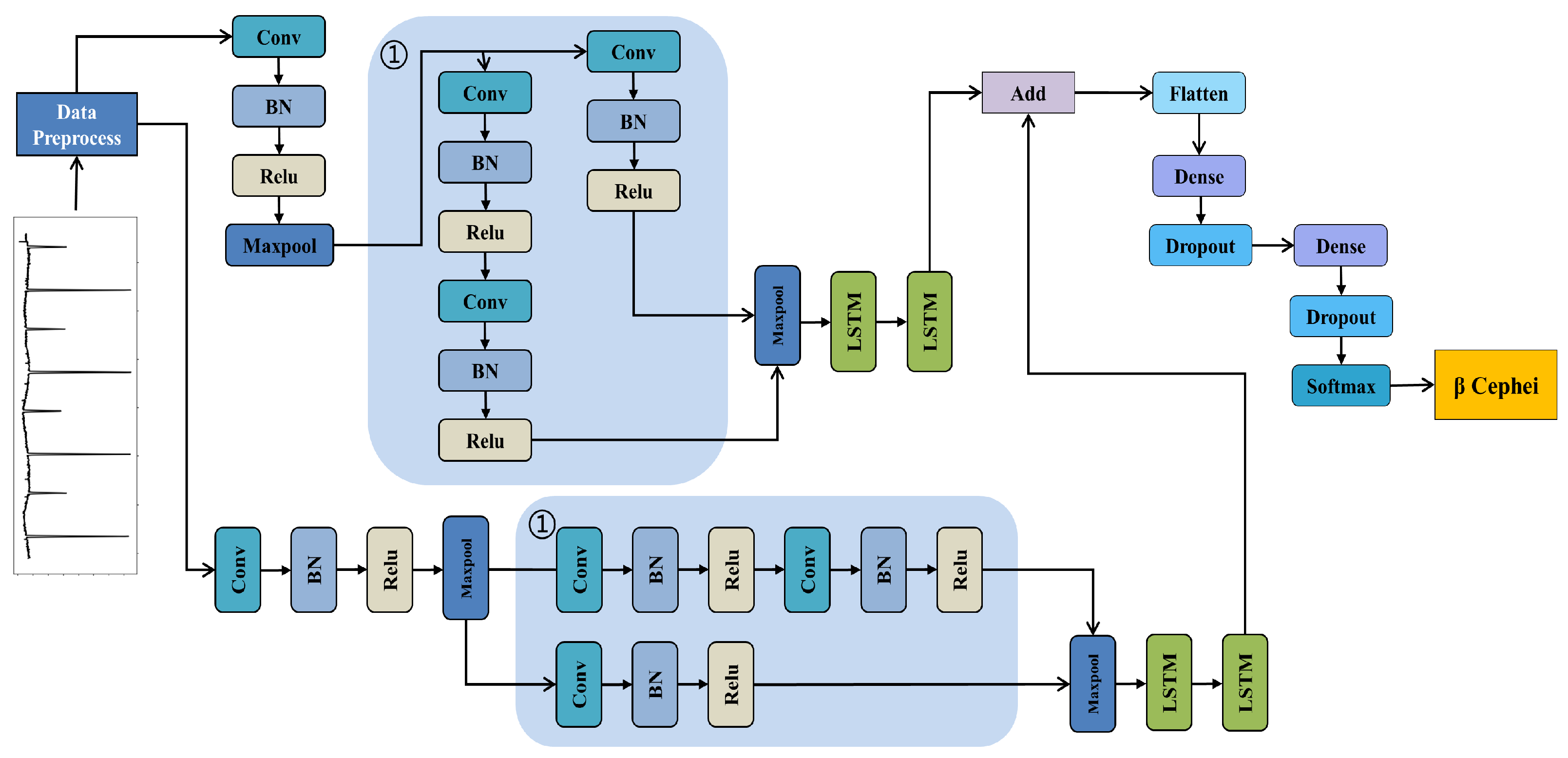
3.1. RLNet
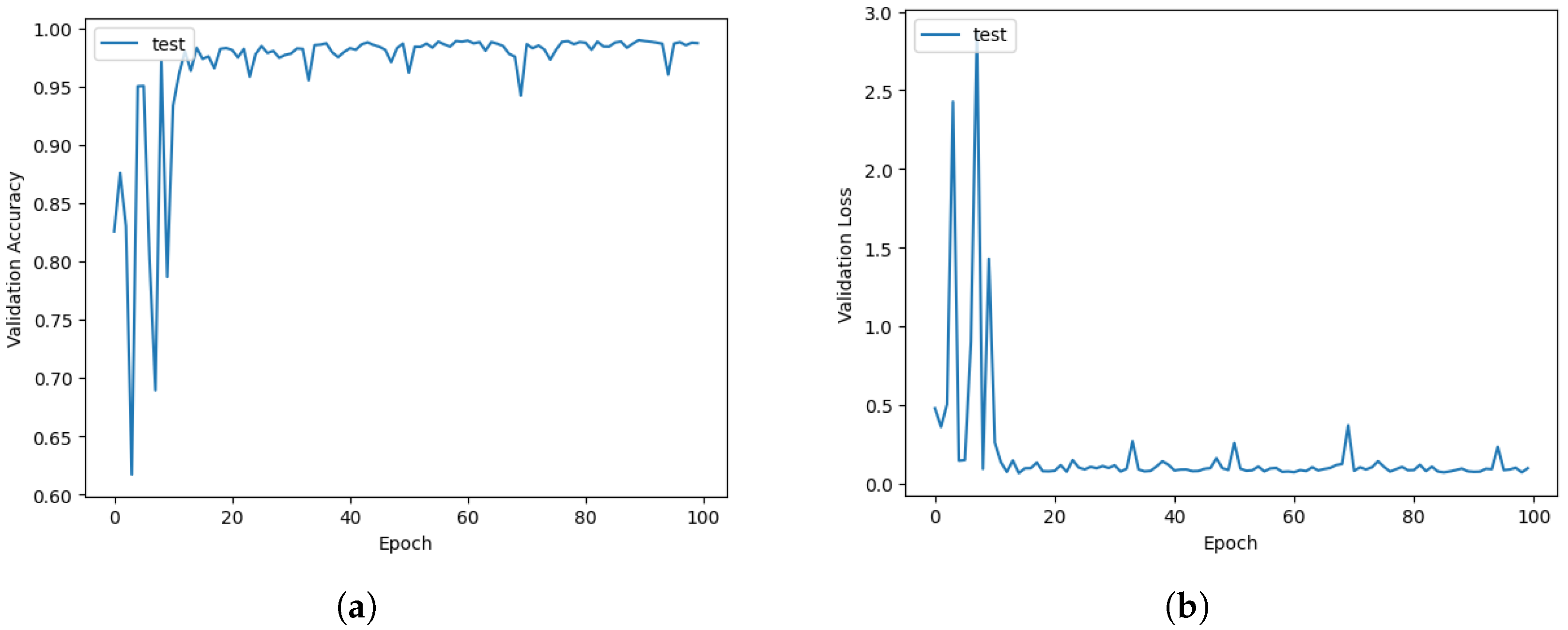
3.2. Training Strategy
- BN layers are added after each convolutional layer. These BN layers normalize the activations of the previous layers, helping to stabilize and accelerate the training process.
- Dropout layers are added after each dense layer. Dropout randomly removes units (along with their connections) from the neural network during training, preventing the units from becoming overly dependent on each other and reducing co-adaptation [29].
4. Results
4.1. Evaluation Metrics
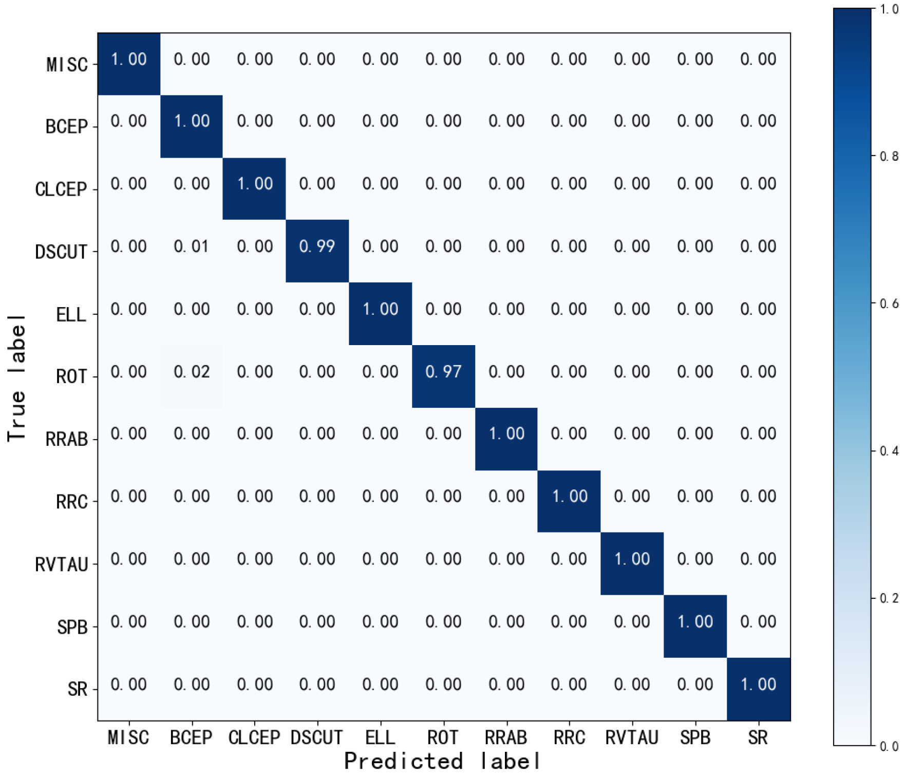
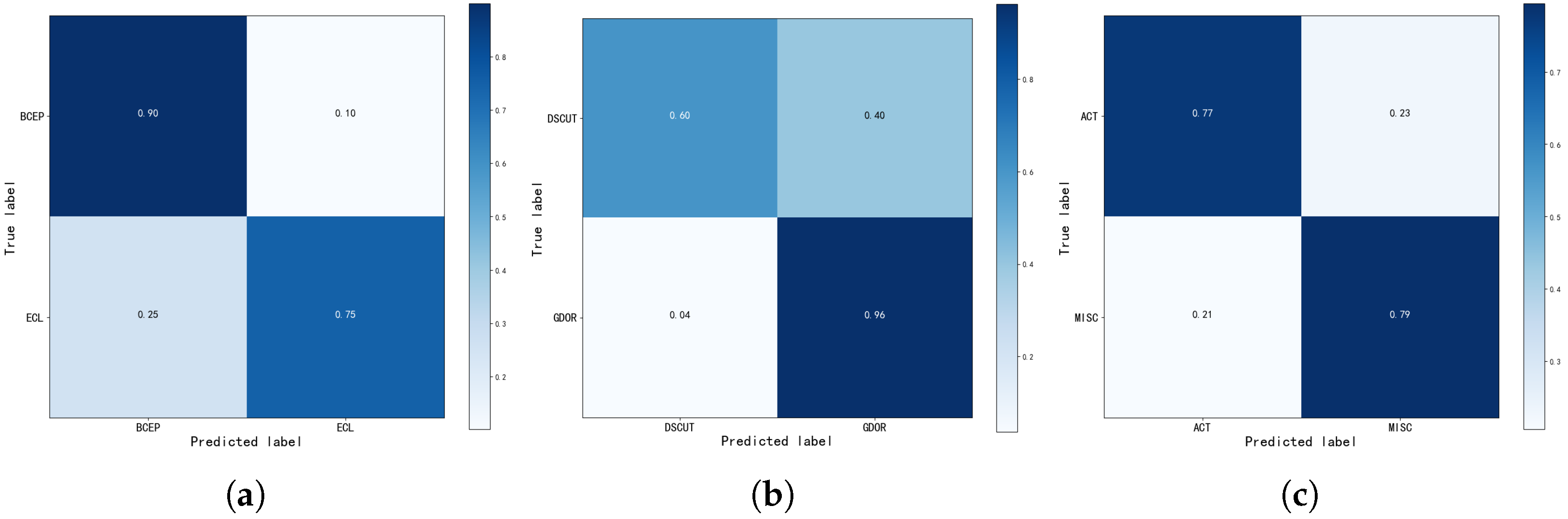
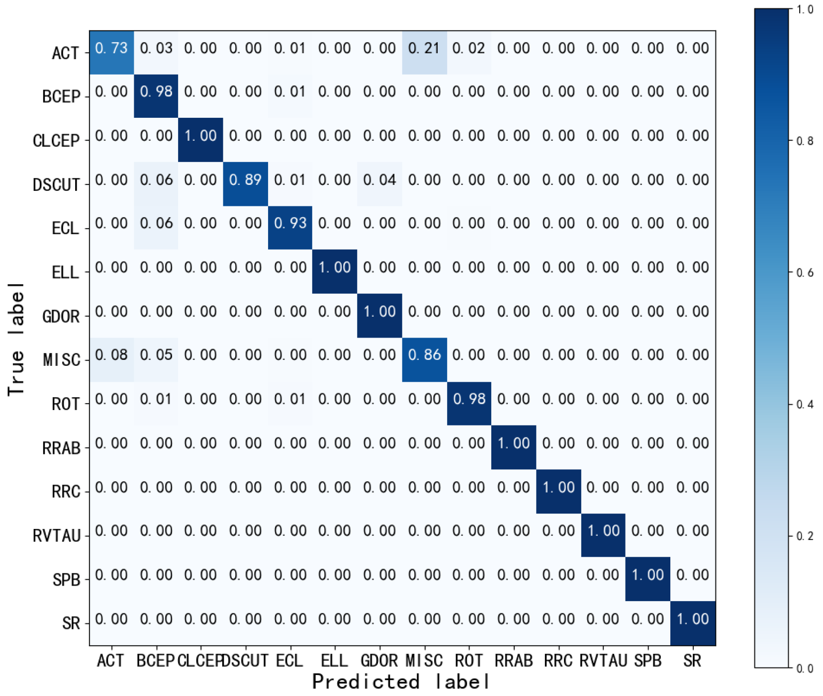
4.1.1. Confusion Matrix
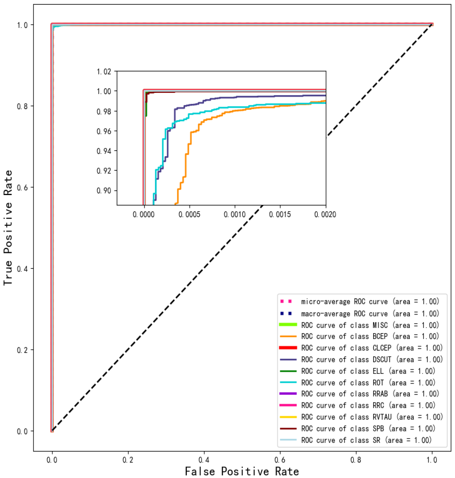
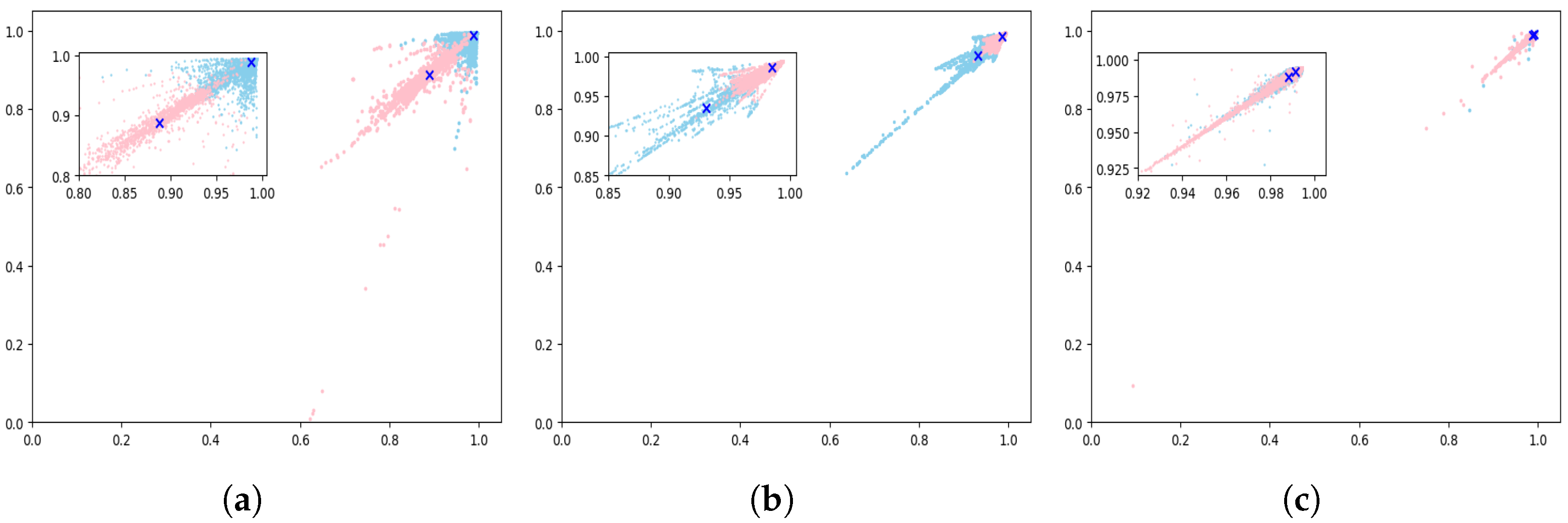
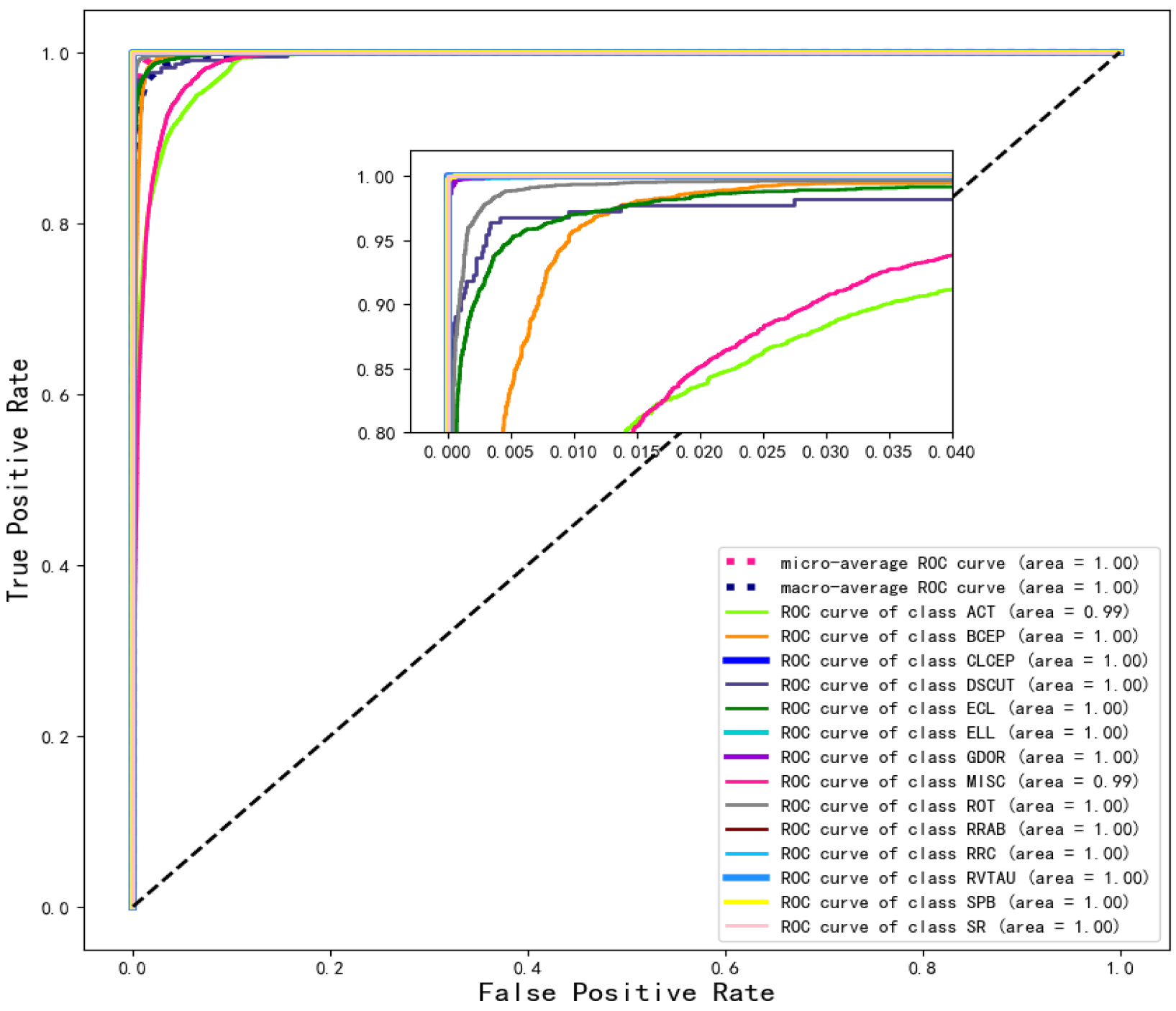
4.1.2. ROC Curve
4.1.3. PR Curve
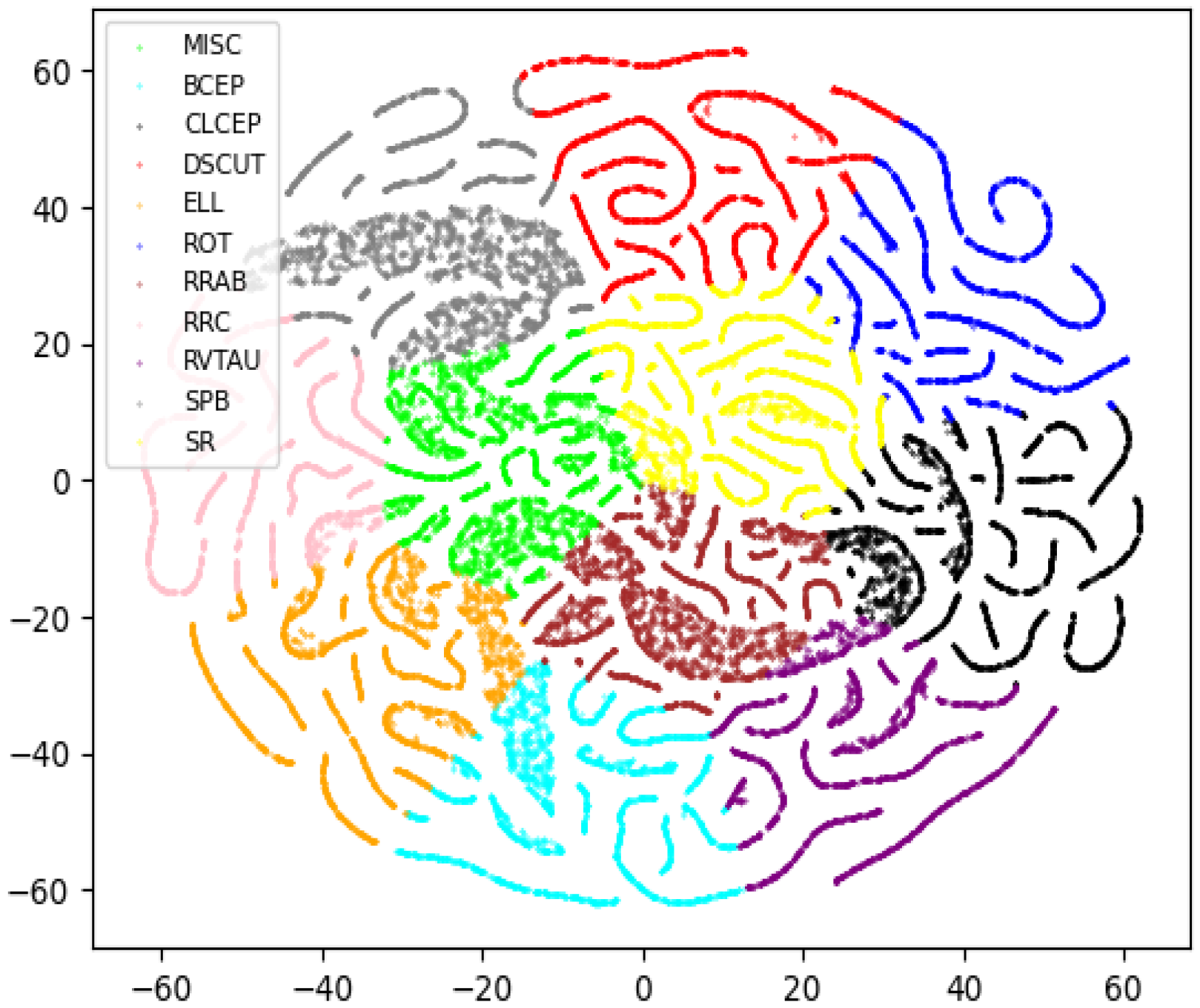
4.2. Representing Light Curves in a High-Dimensional Feature Space
4.3. Clustering Results
4.4. Comparison Experiment
4.4.1. Comparison with Typical Methods
4.4.2. Comparison with Ensemble Classifier
5. Conclusions
Author Contributions
Funding
Data Availability Statement
Conflicts of Interest
References
- Kirk, B.; Conroy, K.; Prša, A.; Abdul-Masih, M.; Kochoska, A.; MatijeviČ, G.; Hambleton, K.; Barclay, T.; Bloemen, S.; Boyajian, T.; et al. Kepler eclipsing binary stars. VII. The catalog of eclipsing binaries found in the entire Kepler data set. Astron. J. 2016, 151, 68. [Google Scholar] [CrossRef]
- Mahabal, A.; Sheth, K.; Gieseke, F.; Pai, A.; Djorgovski, S.; Drake, A.; Graham, M.; Collaboration, C. Deep-learnt classification of light curves. In Proceedings of the 2017 IEEE Symposium Series on Computational Intelligence (SSCI), Honolulu, HI, USA, 27 November–1 December 2017; IEEE: New York, NY, USA, 2017; p. 2757. [Google Scholar]
- Hinners, T.A.; Tat, K.; Thorp, R. Machine learning techniques for stellar light curve classification. Astron. J. 2018, 156, 7. [Google Scholar] [CrossRef]
- Masci, F.J.; Hoffman, D.I.; Grillmair, C.J.; Cutri, R.M. Automated classification of periodic variable stars detected by the wide-field infrared survey explorer. Astron. J. 2014, 148, 21. [Google Scholar] [CrossRef]
- Bass, G.; Borne, K. Supervised ensemble classification of Kepler variable stars. Mon. Not. R. Astron. Soc. 2016, 459, 3721–3737. [Google Scholar] [CrossRef]
- Zinn, J.; Kochanek, C.; Kozłowski, S.; Udalski, A.; Szymański, M.; Soszyński, I.; Wyrzykowski, Ł.; Ulaczyk, K.; Poleski, R.; Pietrukowicz, P.; et al. Variable classification in the LSST era: Exploring a model for quasi-periodic light curves. Mon. Not. R. Astron. Soc. 2017, 468, 2189–2205. [Google Scholar] [CrossRef]
- Sánchez-Sáez, P.; Reyes, I.; Valenzuela, C.; Förster, F.; Eyheramendy, S.; Elorrieta, F.; Bauer, F.; Cabrera-Vives, G.; Estévez, P.; Catelan, M.; et al. Alert classification for the ALeRCE broker system: The light curve classifier. Astron. J. 2021, 161, 141. [Google Scholar] [CrossRef]
- Adassuriya, J.; Jayasinghe, J.; Jayaratne, K. Identifying Variable Stars from Kepler Data Using Machine Learning. Eur. J. Appl. Phys. 2021, 3, 32–35. [Google Scholar] [CrossRef]
- Morales, A.; Rojas, J.; Huijse, P.; Ramos, R.C. A Comparison of Convolutional Neural Networks for RR Lyrae Light Curve Classification. In Proceedings of the 2021 IEEE Latin American Conference on Computational Intelligence (LA-CCI), Temuco, Chile, 2–4 November 2021; IEEE: New York, NY, USA, 2021; pp. 1–6. [Google Scholar]
- Szklenár, T.; Bódi, A.; Tarczay-Nehéz, D.; Vida, K.; Marton, G.; Mező, G.; Forró, A.; Szabó, R. Image-based Classification of Variable Stars: First Results from Optical Gravitational Lensing Experiment Data. Astrophys. J. Lett. 2020, 897, L12. [Google Scholar] [CrossRef]
- Burhanudin, U.; Maund, J.; Killestein, T.; Ackley, K.; Dyer, M.; Lyman, J.; Ulaczyk, K.; Cutter, R.; Mong, Y.; Steeghs, D.; et al. Light-curve classification with recurrent neural networks for GOTO: Dealing with imbalanced data. Mon. Not. R. Astron. Soc. 2021, 505, 4345–4361. [Google Scholar] [CrossRef]
- Demianenko, M.; Samorodova, E.; Sysak, M.; Shiriaev, A.; Malanchev, K.; Derkach, D.; Hushchyn, M. Supernova Light Curves Approximation based on Neural Network Models. J. Phys. Conf. Ser. 2023, 2438, 012128. [Google Scholar] [CrossRef]
- Modak, S.; Chattopadhyay, T.; Chattopadhyay, A.K. Unsupervised classification of eclipsing binary light curves through k-medoids clustering. J. Appl. Stat. 2020, 47, 376–392. [Google Scholar] [CrossRef] [PubMed]
- Armstrong, D.; Kirk, J.; Lam, K.; McCormac, J.; Osborn, H.; Spake, J.; Walker, S.; Brown, D.; Kristiansen, M.; Pollacco, D.; et al. K2 variable catalogue—II. Machine learning classification of variable stars and eclipsing binaries in K2 fields 0–4. Mon. Not. R. Astron. Soc. 2015, 456, 2260–2272. [Google Scholar] [CrossRef]
- Bassi, S.; Sharma, K.; Gomekar, A. Classification of variable stars light curves using long short term memory network. Front. Astron. Space Sci. 2021, 8, 718139. [Google Scholar] [CrossRef]
- Barbara, N.H.; Bedding, T.R.; Fulcher, B.D.; Murphy, S.J.; Van Reeth, T. Classifying Kepler light curves for 12 000 A and F stars using supervised feature-based machine learning. Mon. Not. R. Astron. Soc. 2022, 514, 2793–2804. [Google Scholar] [CrossRef]
- Alves, C.S.; Peiris, H.V.; Lochner, M.; McEwen, J.D.; Allam, T.; Biswas, R.; Collaboration, L.D.E.S. Considerations for optimizing the photometric classification of supernovae from the rubin observatory. Astrophys. J. Suppl. Ser. 2022, 258, 23. [Google Scholar] [CrossRef]
- Daubechies, I. The wavelet transform, time-frequency localization and signal analysis. IEEE Trans. Inf. Theory 1990, 36, 961–1005. [Google Scholar] [CrossRef]
- Rhif, M.; Ben Abbes, A.; Farah, I.R.; Martínez, B.; Sang, Y. Wavelet transform application for/in non-stationary time-series analysis: A review. Appl. Sci. 2019, 9, 1345. [Google Scholar] [CrossRef]
- McWhirter, P.R.; Steele, I.A.; Al-Jumeily, D.; Hussain, A.; Vellasco, M.M. The classification of periodic light curves from non-survey optimized observational data through automated extraction of phase-based visual features. In Proceedings of the 2017 International Joint Conference on Neural Networks (IJCNN), Anchorage, AK, USA, 14–19 May 2017; IEEE: New York, NY, USA, 2017; pp. 3058–3065. [Google Scholar]
- LeCun, Y.; Bengio, Y.; Hinton, G. Deep learning. Nature 2015, 521, 436–444. [Google Scholar] [CrossRef]
- Pasquet, J.; Pasquet, J.; Chaumont, M.; Fouchez, D. Pelican: Deep architecture for the light curve analysis. Astron. Astrophys. 2019, 627, A21. [Google Scholar] [CrossRef]
- He, K.; Zhang, X.; Ren, S.; Sun, J. Deep residual learning for image recognition. In Proceedings of the IEEE Conference on Computer Vision and Pattern Recognition, Las Vegas, NV, USA, 27–30 June 2016; pp. 770–778. [Google Scholar]
- Charnock, T.; Moss, A. Deep recurrent neural networks for supernovae classification. Astrophys. J. Lett. 2017, 837, L28. [Google Scholar] [CrossRef]
- Gers, F.A.; Schmidhuber, J.; Cummins, F. Learning to forget: Continual prediction with LSTM. Neural Comput. 2000, 12, 2451–2471. [Google Scholar] [CrossRef] [PubMed]
- Yu, Y.; Si, X.; Hu, C.; Zhang, J. A review of recurrent neural networks: LSTM cells and network architectures. Neural Comput. 2019, 31, 1235–1270. [Google Scholar] [CrossRef] [PubMed]
- Zhang, R.; Zou, Q. Time series prediction and anomaly detection of light curve using lstm neural network. J. Phys. Conf. Ser. 2018, 1061, 012012. [Google Scholar] [CrossRef]
- Ying, X. An overview of overfitting and its solutions. J. Phys. Conf. Ser. 2019, 1168, 022022. [Google Scholar] [CrossRef]
- Srivastava, N.; Hinton, G.; Krizhevsky, A.; Sutskever, I.; Salakhutdinov, R. Dropout: A simple way to prevent neural networks from overfitting. J. Mach. Learn. Res. 2014, 15, 1929–1958. [Google Scholar]
- Bock, S.; Weiß, M. A proof of local convergence for the Adam optimizer. In Proceedings of the 2019 International Joint Conference on Neural Networks (IJCNN), Budapest, Hungary, 14–19 July 2019; IEEE: New York, NY, USA, 2019; pp. 1–8. [Google Scholar]
- Shi, J.H.; Qiu, B.; Luo, A.L.; He, Z.D.; Kong, X.; Jiang, X. A photometry pipeline for SDSS images based on convolutional neural networks. Mon. Not. R. Astron. Soc. 2022, 516, 264–278. [Google Scholar] [CrossRef]
- Heydarian, M.; Doyle, T.E.; Samavi, R. MLCM: Multi-label confusion matrix. IEEE Access 2022, 10, 19083–19095. [Google Scholar] [CrossRef]
- Fawcett, T. An introduction to ROC analysis. Pattern Recognit. Lett. 2006, 27, 861–874. [Google Scholar] [CrossRef]
- Bradley, A.P. The use of the area under the ROC curve in the evaluation of machine learning algorithms. Pattern Recognit. 1997, 30, 1145–1159. [Google Scholar] [CrossRef]
- Hanley, J.A.; McNeil, B.J. The meaning and use of the area under a receiver operating characteristic (ROC) curve. Radiology 1982, 143, 29–36. [Google Scholar] [CrossRef] [PubMed]
- Kirzhevsky, A.; Sutskever, I.; Hinton, G.E. Imagenet classification with deep convolutional neural networks. Adv. Neural Inf. Process. Syst. 2012, 25, 1097–1105. [Google Scholar] [CrossRef]
- Muthukrishna, D.; Narayan, G.; Mandel, K.S.; Biswas, R.; Hložek, R. RAPID: Early classification of explosive transients using deep learning. Publ. Astron. Soc. Pac. 2019, 131, 118002. [Google Scholar] [CrossRef]
- Linares, R.; Furfaro, R.; Reddy, V. Space objects classification via light-curve measurements using deep convolutional neural networks. J. Astronaut. Sci. 2020, 67, 1063–1091. [Google Scholar] [CrossRef]
- Davis, J.; Goadrich, M. The relationship between Precision-Recall and ROC curves. In Proceedings of the 23rd International Conference on Machine Learning, Pittsburgh, PA, USA, 25–29 June 2006; pp. 233–240. [Google Scholar]
- Juba, B.; Le, H.S. Precision-recall versus accuracy and the role of large data sets. In Proceedings of the AAAI Conference on Artificial Intelligence, Honolulu, HI, USA, 27 January–1 February 2019; Volume 33, pp. 4039–4048. [Google Scholar]
- Blomme, J.; Sarro, L.; O’Donovan, F.; Debosscher, J.; Brown, T.; Lopez, M.; Dubath, P.; Rimoldini, L.; Charbonneau, D.; Dunham, E.; et al. Improved methodology for the automated classification of periodic variable stars. Mon. Not. R. Astron. Soc. 2011, 418, 96–106. [Google Scholar] [CrossRef]


| Abbreviation | Class | Original Number | Balanced Number | Final Number |
|---|---|---|---|---|
| ACT | Activity | 18,250 | 19,874 | |
| BCEP | Cephei | 18,254 | 19,956 | 38,386 |
| CLCEP | Classical Cepheids | 18 | 19,992 | 19,992 |
| DSCUT | Scuti | 884 | 1137 | 1137 |
| ECL | Eclipsing variables | 2322 | 18,430 | |
| ELL | Ellipsoida | 191 | 19,881 | 19,881 |
| GDOR | Doradus | 424 | 19,712 | |
| MISC | Miscellaneous/No-variable | 90,388 | 20,000 | 39,874 |
| ROT | Rotating | 7718 | 17,694 | 17,694 |
| RRAB | RR Lyrae type AB | 4 | 8001 | 8001 |
| RRC | RR Lyrae type C | 16 | 19,998 | 19,998 |
| RVTAU | RVTauri | 3 | 3928 | 3928 |
| SPB | Slowly pulsating B star | 371 | 19,840 | 19,840 |
| SR | Semiregular | 4 | 3991 | 3991 |
| Attribute Name | Description |
|---|---|
| IMAG | Sloan I magnitude |
| JMAG | 2MASS J magnitude |
| KMAG | Sloan K magnitude |
| TEFF | Effective surface temperature |
| G.R.color | G-R color |
| Radius | Stellar radius |
| Log G | log 10 of the surface gravity |
| Std | Standard deviation of the flux |
| Median | Median of the flux |
| Skew | Statistical skewness of the flux distribution |
| Kurtosis | Statistical kurtosis (peakedness) of the flux |
| Beyond1st | Fraction of all data points above the first standard deviation of flux |
| SSDev | Sum of the square of the difference of the flux from the median flux |
| Dimensionality | 65 | 115 | 217 | 419 | |
|---|---|---|---|---|---|
| Method | |||||
| Fourier transform | 27% | 62% | 71.6% | 89% | |
| Wavelet transform | 72% | 98.7% | 97.6% | 96% | |
| Method | Accuracy |
|---|---|
| Random forest | 0.767 |
| AlexNet (2012) [36] | 0.741 |
| Mahabal et al. (2017) [2] | 0.401 |
| Muthukrishna et al. (2019) [37] | 0.780 |
| Linares et al. (2020) [38] | 0.768 |
| Szklenár et al. (2020) [10] | 0.254 |
| Morales et al. (2021) [9] | 0.934 |
| Ours | 0.987 |
| Category | MISC | BCEP | CLCEP | DSCUT | ELL | ROT | RRAB | RRC | RVTAU | SPB | SR | |
|---|---|---|---|---|---|---|---|---|---|---|---|---|
| Precision | ||||||||||||
| Random forest | 0.999 | 0.685 | 0.848 | 0.612 | 0.589 | 0.654 | 0.999 | 0.831 | 0.995 | 0.570 | 0.001 | |
| AlexNet (2012) [36] | 0.997 | 0.472 | 0.995 | 0.723 | 0.903 | 0.398 | 0.998 | 0.998 | 0.999 | 0.850 | 0.001 | |
| Mahabal et al. (2017) [2] | 0.394 | 0.110 | 0.481 | 0.607 | 0.304 | 0.182 | 0.969 | 0.559 | 0.001 | 0.376 | 0.001 | |
| Muthukrishna et al. (2019) [37] | 0.680 | 0.492 | 0.999 | 0.872 | 0.953 | 0.824 | 0.999 | 0.999 | 0.999 | 0.972 | 0.985 | |
| Linares et al. (2020) [38] | 0.499 | 0.593 | 0.997 | 0.821 | 0.911 | 0.779 | 0.999 | 0.994 | 0.998 | 0.905 | 0.838 | |
| Szklenár et al. (2020) [10] | 0.001 | 0.230 | 0.431 | 0.001 | 0.001 | 0.001 | 0.244 | 0.001 | 0.001 | 0.001 | 0.001 | |
| Morales et al. (2021) [9] | 0.999 | 0.892 | 0.998 | 0.791 | 0.894 | 0.913 | 0.999 | 0.998 | 0.996 | 0.898 | 0.995 | |
| Ours | 0.999 | 0.978 | 0.999 | 0.973 | 0.995 | 0.970 | 0.999 | 0.999 | 0.999 | 0.999 | 0.994 | |
| Category | MISC | BCEP | CLCEP | DSCUT | ELL | ROT | RRAB | RRC | RVTAU | SPB | SR | |
|---|---|---|---|---|---|---|---|---|---|---|---|---|
| Recall | ||||||||||||
| Random forest | 0.999 | 0.820 | 0.884 | 0.420 | 0.404 | 0.745 | 0.999 | 0.999 | 0.822 | 0.632 | 0.001 | |
| AlexNet (2012) [36] | 0.958 | 0.748 | 0.939 | 0.283 | 0.629 | 0.639 | 0.999 | 0.875 | 0.979 | 0.648 | 0.001 | |
| Mahabal et al. (2017) [2] | 0.990 | 0.035 | 0.594 | 0.018 | 0.256 | 0.001 | 0.629 | 0.664 | 0.001 | 0.770 | 0.001 | |
| Muthukrishna et al. (2019) [37] | 0.513 | 0.784 | 0.950 | 0.705 | 0.849 | 0.777 | 0.999 | 0.992 | 0.994 | 0.846 | 0.584 | |
| Linares et al. (2020) [38] | 0.806 | 0.213 | 0.999 | 0.792 | 0.925 | 0.728 | 0.999 | 0.999 | 0.999 | 0.940 | 0.999 | |
| Szklenár et al. (2020) [10] | 0.001 | 0.940 | 0.512 | 0.001 | 0.001 | 0.001 | 0.999 | 0.001 | 0.001 | 0.001 | 0.001 | |
| Morales et al. (2021) [9] | 0.999 | 0.859 | 0.995 | 0.895 | 0.882 | 0.828 | 0.999 | 0.999 | 0.999 | 0.923 | 0.997 | |
| Ours | 0.999 | 0.971 | 0.999 | 0.989 | 0.995 | 0.968 | 0.999 | 0.999 | 0.999 | 0.999 | 0.999 | |
Disclaimer/Publisher’s Note: The statements, opinions and data contained in all publications are solely those of the individual author(s) and contributor(s) and not of MDPI and/or the editor(s). MDPI and/or the editor(s) disclaim responsibility for any injury to people or property resulting from any ideas, methods, instructions or products referred to in the content. |
© 2023 by the authors. Licensee MDPI, Basel, Switzerland. This article is an open access article distributed under the terms and conditions of the Creative Commons Attribution (CC BY) license (https://creativecommons.org/licenses/by/4.0/).
Share and Cite
Yan, J.; Wu, H.; Qiu, B.; Luo, A.-L.; Ren, F. Feature-Based Classification Neural Network for Kepler Light Curves from Quarter 1. Universe 2023, 9, 435. https://doi.org/10.3390/universe9100435
Yan J, Wu H, Qiu B, Luo A-L, Ren F. Feature-Based Classification Neural Network for Kepler Light Curves from Quarter 1. Universe. 2023; 9(10):435. https://doi.org/10.3390/universe9100435
Chicago/Turabian StyleYan, Jing, Huanli Wu, Bo Qiu, A-Li Luo, and Fuji Ren. 2023. "Feature-Based Classification Neural Network for Kepler Light Curves from Quarter 1" Universe 9, no. 10: 435. https://doi.org/10.3390/universe9100435
APA StyleYan, J., Wu, H., Qiu, B., Luo, A.-L., & Ren, F. (2023). Feature-Based Classification Neural Network for Kepler Light Curves from Quarter 1. Universe, 9(10), 435. https://doi.org/10.3390/universe9100435