1. Introduction
Since the discovery that black holes would have to emit radiation, there have been proposals to explain the loss of information associated with the apparent conversion of pure to mixed quantum states. From the beginning, this information loss was proposed to be fundamental and, the non unitary evolution of pure to mixed quantum states constituted a hypothesis to solve the problem associated with this loss. For example, Steven Hawking own proposal of the non unitary evolution is represented by the “dollar matrix”
[
1]
which allows the evolution of pure quantum states, characterised by the density matrix
, into mixed states
.
The black hole evaporation mechanism and the problem of information loss, collected behind the event horizon, constituted a privileged arena for quantum gravity theories candidates (namely, quantum geometrodynamics [
2], string theory [
3,
4,
5,
6,
7] and loop quantum gravity [
8,
9,
10,
11]) to establish themselves beyond General Relativity. However, the scientific community was reluctant to give up unitarity, a crucial feature of Quantum Mechanics, and the hypothesis of a new principle of complementarity, between the points of views of an infinitely distant observer and a free falling observer near the event horizon, was raised [
12]. Following a similar approach, it has been emphasised over the time the role of the gravitational back reaction effect [
13,
14] of Hawking radiation on the event horizon as a way to allow the information accumulated within the black hole to be encoded in the outgoing radiation. In this way, the emergence of a mechanism in which all the black hole information (a four dimensional object in General Relativity) would be accessible at the event horizon (which can be described as a membrane with one dimension less than the black hole), is somehow similar to what happens with a hologram [
15]. This new holographic principle was simultaneously proposed and clarified [
16,
17] in order to incorporate the aforementioned principle of complementarity. The next step happened when it was conjectured the correspondence between classes of quantum gravity theories (5-dimensional anti-De Sitter solutions in string theories) and conformal field theory (CFT-conformal field theory-4-dimensional boundary of the 5-dimensional solutions), the so called AdS/CFT conjecture [
18,
19,
20,
21]. This discovery was extremely important to ensure the possibility of a correspondence between the physics that describes the interior of the black hole (supposedly quantum gravity), and the existence of a quantum field theory at its boundary (the surface that defines the event horizon) that would allow to save the unitarity.
In 2012, in an effort to analyse important assumptions, such as: (1) the principle of complementarity proposed by Susskind and its colaborators, (2) the AdS/CFT correspondence and, (3) the equivalence principle of General Relativity, in the way that Hawking radiation could encode the information stored in the black hole, a new paradox was discovered [
22]. In simple terms, the impossibility of having the particle, which leaves the black hole, in an maximally entangled state (or non factored state) with two systems simultaneously (the pair disappearing beyond the horizon and all the Hawking radiation emitted in the past, a problem related to the so-called monogamy of entanglement), leads to postulate the existence of a firewall that would destroy any free falling observer trying to cross the event horizon. The firewall existence is incompatible with Einstein’s equivalence principle. However, if there is no firewall, and the principle of equivalence is respected, according to these authors, unitarity is lost and information loss is inevitable. Apparently, the situation is such that either General Relativity principles or Quantum Mechanics principles need to be reviewed [
23,
24]. This is an open problem and the role of gravitational back reaction, between Hawking radiation and the black hole, persists as an unknown and potentially enlightening mechanism on how to correctly formulate a quantum theory of the gravitational field.
In an attempt to study the possible gravitational back reaction, between Hawking radiation and the black hole, from the quantum geometrodynamics point of view, a toy model was proposed [
25]. It was shown and discussed the conditions under which the Wheeler-DeWitt equation could be used to describe a quantum black hole. In particular, a simple model for the black hole evaporation was studied using a Schrödinger type of equation and, the cases for initial squeezed ground states and coherent states were taken to represent the initial black hole quantum state. One can ask, how can a complex equation such as the Wheeler-DeWitt be approximated by a Schrödinger type of equation? In the cosmological context, several formal derivations were carried [
2,
26,
27,
28,
29] with the purpose of enabling to use the limit of a quantum field theory in an external space-time for the full quantum gravity theory. Such approaches usually involve procedures like the Born-Oppenheimer or Wentzel-Kramers-Brillouin (WKB) approximations.
In this work we review this toy model. It is important to notice that, even though, a full study of the time evolution of the Hawking radiation and black hole quantum states was performed when a simple back reaction term is introduced, an important part of the discussion about the time evolution of the resulting entangled state was left incomplete. In fact, it is exactly the motivation of this paper to address the problem of explicitly describe the time evolution of the degree of entanglement of this quantum system. In addition, another important goal is to get an approximate estimate of the Von Neumann entropy and check is the back reaction can induce a release of the quantum information in the Hawking radiation. These results can be interesting, in the quantum geometrodynamics context, as a simple starting point to more robustly address the black hole information paradox in a canonical quantization of gravity program.
This paper is organized as follow. In
Section 2 and
Section 3 we present an introduction to quantum geometrodynamics and consider a semiclassical approximation of the Wheeler-DeWitt equation. In
Section 4 and
Section 5 we derive a simple model of the back reaction between the Hawking radiation and the black hole quantum states, where its dynamics is governed by a Schrödinger type of equation. Finally, in
Section 6 and
Section 7, we obtain and discuss the main result of this paper, namely the time evolution of the entanglement entropy and the behaviour of the quantum information of the Hawking radiation state.
2. Quantum Geometrodynamics and the Semiclassical Approximation
In the following, we mention a brief description of the bases of J.A. Wheeler’s geometrodynamics, which consists in a 3 + 1 spacetime decomposition (ADM decomposition-R. Arnowitt, S. Deser and C.W. Misner [
30]), and obtain General Relativity field equations in that context. The field equations, obtained in this procedure, will exhibit the evolution of a pair of dynamical variables
-the 3-dimensional metric
(induced metric) and the extrinsic curvature
-on a Cauchy hypersurface
(three-dimensional surface).
General Relativity, defined by the Einstein-Hilbert action, here without the cosmological constant,
can be expressed under the hamiltonian formalism. For this purpose, a
decomposition of spacetime
1 may be considered, where
is a smooth manifold and
g lorentzian metric in
. Moreover, this decomposition consists of the 4-dimensional spacetime foliation in a continuous sequence of Cauchy hypersurfaces
, parameterised by a global time variable
t2. General Relativity covariance is maintained, in this procedure, by considering all possible ways of carrying this foliation. When we consider the hamiltonian formalism we need to define a pair of canonical variables, however, we can initially identify a pair of dynamical variables constituted, on the one hand, by the 3-dimensional metric induced in
by the spacetime metric
where
is an ortogonal vector to
. In this way we can separate the metric
g, in its temporal e spatial components, according to the following expressions,
or, in a more suitable compact form,
In the previous equation
N is called the lapse function whereas
is the shift vector. The other canonical variable, on the other hand, is the extrinsic curvature
Hence, the dynamical variables pair
(with Latin letter indexes, defining 3-dimensional tensor fields) enable us to rewrite Einstein-Hilbert action (
1) as
We can notice that the lapse function and the shift vector are Lagrange multipliers (since
e
) and, according to Dirac [
31] we can establish the existence of primary constraints which allow to write the action (
6) as
with
(conjugate momentum of the dynamical variable
) and where
with
being the DeWitt metric and
is the covariant derivative. We can define the hamiltonian constraint
and the diffeomorphism constraint
through the variation of the action (
7) with respect to
N and
. Physically, constraints (
9)–(
10) express the freedom to choose any coordinate system in General Relativity. More precisely, the choice of the particular foliation
is equivalent to choose the lapse function
N and, the spatial coordinates
choice is equivalent to choose a particular shift vector
. It is important to emphasise that, related to the DeWitt metric
definition, the kinetic term in Equation (
9) is indefinite, since not all kinetic functional operators in Equation (
8) share the same sign. This property will persist beyond the quantisation procedure and will play a crucial role in the semiclassical (where it will give rise to a negative kinetic term) approach to the black hole evaporation process.
3. Canonical Variables Quantisation and Wheeler-DeWitt Equation
The canonical quantisation programme, according to P.M. Dirac prescription, demands the transition of classical to quantum canonical variables , and also promotes Poisson brackets to commutators. We have to define a wave state functional belonging to the space of all 3-dimensional metrics Riem . Nevertheless, there are important issues related with:
the correct factor ordering in building quantum observables from the fundamental variables ,
the interpretation of quantum observables as operators acting on the wave functional and the adequate definition of a Hilbert space,
the classical constraints (
9)–(
10) conversion to their quantum counterpart
and their quantum interpretation,
the lack of time evolution in the previous quantum constraints.
These questions are thoroughly discussed in [
2,
32], as well as possible solutions and open problems till the present day. Among the previous mentioned issues, the problem related to the lack of time evolution seems to stand as an essential feature in the formulation of a quantum theory of the gravitational field. If we assume that the wave functional evolution over time depends on a time concept defined after the canonical quantisation, then, the time parameter
t will be an emergent quantity [
33].
In order to address the black hole evaporation problem and, to explore how information is eventually encoded in Hawking radiation, it would be important to obtain the entropy time evolution as a measure of the degree of quantum entanglement between radiation and black hole states. Since the quantum version of the hamiltonian constraint (
9),
known as Wheeler-DeWitt equation, and the quantum diffeomorphism constraint
are both time independent, the wave functional is connected to a purely quantum and closed gravitational system. In the case involving the study of a black hole evaporation phase, Equations (
12) and (
13) describe a quantum black hole in the context of a purely quantum universe. This situation is not suitable if we consider that we must have several classical observers measuring and depicting the time evolution of the black hole outgoing radiation. These classical observers, experience and describe physical phenomena in a classical language that needs a time parameter. Hence, we need to consider a quantum black hole in a semiclassical universe where time appears as an emergent quantity.
Time is the product of an approximation which aims to extract, from the Wheeler-DeWitt equation, an external, semiclassical stage, in which black hole and Hawking radiation quantum states evolve.
In reference [
2] (Section 5.4) we can find a derivation, from Equations (
12) and (
13), of a Schrödinger functional equation. In the following, we highlight some important details of this derivation. Let us start by writing the wave functional as
where
is a solution of the vacuum Einstein-Hamilton-Jacobi function [
34], since its WKB approximation enable us to extract, at higher orders, a Hamilton-Jacobi equation. In addition,
is also solution to the Hamilton-Jacobi version of (
12)–(
13), namely
with the definitions
,
and
and
are assumed to be contributions from the non-gravitational fields. Having the solution
, we can now evaluate
along a solution of the classical Einstein equations
. In fact this solution is obtained from
after a choice of the lapse and shift function has been made. At this point, we can define the evolutionary equation for the quantum state
as
which, since
depends on the DeWitt metric
, will have differential operators with the wrong sign in its right hand side. Finally, we are in the position of defining a functional Schrödinger equation for quantized matter fields in an external classical gravitational field as
Notice that the matter hamiltonian , is parametrically depending on metric coefficients of the curved space-time background and contain indefinite kinetic terms.
This derivation assumes a separation of the complete system (which state obeys the Wheeler-DeWitt equation and the quantum diffeomorphism invariance) in two parts, in total correspondence with the way a Born-Oppenheimer approximation is implemented. The physical system separation into two parts, one purely quantum and the other semiclassical, is essentially achieved by separating the gravitational from the non gravitational degrees of freedom through an expansion, with respect to the Planck mass
, of constraints (
12)–(
13). However, we notice that there are gravitational degrees of freedom that can be included in the purely quantum part (quantum density fluctuations whose origin is gravitational, for example). Equation (
19), formally similar to Schrödinger equation, is an equation with functional derivatives, in which variable
is related to the 3-dimensional metric
. As previously mentioned, we recall that due to the DeWitt
metric definition, a negative kinetic term emerges from the conjugated momentum
.
In the following section, let us develop a simple model of the black hole evaporation stage [
25], which incorporates one interesting feature of the Wheeler-DeWitt equation, namely the indefinite kinetic term, and study some of its consequences. The main objective, here, is to estimate the degree of entanglement between Hawking radiation and black hole quantum states, when we take into account a simple form of back reaction between the two.
4. Simplified Model with a Schrödinger Type of Equation
Equation (
19) is a functional differential equation, its wave functional solution depends on the 3-metric
describing the black hole and matter fields. It is obviously an almost impossible task to solve and find solutions to that equation. However, we can consider a simpler model, assuming a Schrödinger type of equation, which was first considered in [
2]. In that work it was argued that in order to study the effect of the indefinite kinetic term in (
19), as a first approach, and since we are dealing with an equation which is formally a Schrödinger equation, we could restrict our attention to finite amount of degrees of freedom. This first approach as been successful in cosmology, allowing to solve the Wheeler-DeWitt equation in minisuperspace, which brings a functional differential equation to a regular differential equation. We do not claim that we are doing the exact same process, but instead that a reduction of the physical system to a finite number of degrees of freedom could retain some aspects of quantum gravity that could be studied using much simpler equations. It is an acceptable concern if approximating a functional differential equation to a Schrödinger type of regular differential equation becomes an oversimplification. Nevertheless, it can also be acceptable to think that some physical insight can be obtained by assuming that the indefinite character of the functional equation is mimicked in the simpler model. Let us consider some assumptions in order to obtain the simpler equation.
Assuming that the hamiltonian
includes black hole and Hawking radiation parts, and ignoring other degrees of freedom, the simpler equation can take the form,
This last equation, where the emergence of a negative kinetic term which plays the role of the functional derivative in the metric
in (
12), contrasts with an exact Schrödinger equation. Therefore, because variable
x is related to metric
, we propose to identify it with the variation of the black hole radius
3 , which turn out to be also a variation in the black hole mass or energy. Variable
y will correspond to Hawking radiation with energy
.
Notice that the kinetic term of the gravitational part of the hamiltonian operator is suppressed by the Planck mass. As long as the black hole mass is large, this kinetic term is irrelevant. One would have in that case, only the Hawking radiation contribution. If, instead we consider the last stages of the evaporation process, when the black hole mass approaches the Planck mass, then the kinetic term associated with the black hole state becomes relevant.
The time parameter
t in Equation (
20) was obtained by means of a Born-Oppenheimer approximation and embodies all the semiclassical degrees of freedom of the universe.
In Equation (
20) we consider harmonic oscillator potentials. Beside being simpler potentials, they allow for analytical solutions and, in the Hawking radiation case this regime is realistic [
35,
36]. For the black hole, this potential is an oversimplification, which can be far from realistic. However, it can help to disclose behaviours also present among more complex potentials, with respect to the entanglement between black hole and Hawking radiation quantum states, during the evaporation process. Furthermore, before dealing with the full problem, simpler models can identify physical phenomena that will reasonably manifest independently of the problem complexity (for example, the infinite square well helps to understand energy quantisation in the more complex Coulomb potential).
Let us assume that Equation (
20) is solved by the variables separation method,
so that we can obtain the two following equations
4,
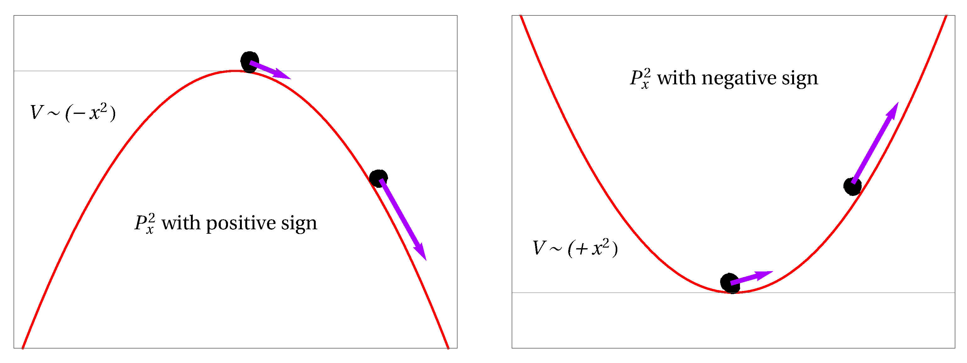
Equations (
22) describe an uncoupled system comprising a harmonic oscillator and an inverted one. In
Figure 1 we illustrate the fact that having regular harmonic potential with a negative (indefinite) kinetic term is equivalent, in the quantum point of view, to the situation where an inverted oscillator potential has a positive kinetic term. In both situations we have to deal with an unstable system, which would correspond of having variable
x varying uncontrollably. A wave function
that initially has a Gaussian profile, will evolve over time according to,
where
is the inverted oscillator Green function [
37,
38],
which can be obtained from the harmonic oscillator Green function
by redefining
. The wave function obtained from the computation of Equation (
23) shows a progressive squeezing of the state in phase space, which means an increasing uncertainty in the value of
x. Physically, in this simplified model, that would correspond to an unstable variation of the Schwarzschild radius or mass of the black hole. Even though, conceivably, a strong squeezing of the black hole state would occur [
39], driving its disappearance.
In the next section we will introduce the effect of a back reaction, coupling effectively black hole and Hawking radiation quantum states, and see that, under particular circumstances, the system becomes stable and strongly entangled.
5. Back Reaction and Schrödinger Equation
In this section we review and reproduce some results obtained in reference [
25]. Notice that in this work a slight change in some definitions will be carried. In addition some new aspects of the model will be discussed. In order to investigate the effects of a back reaction between Hawking radiation and black hole states, let us consider a linear coupling
between the variables, where
is a constant, in equation
We should emphasize that, following the Born-Oppenheimer and WKB approximation used to obtain Equation (
19), any phenomenological back reaction effect, here parametrized by
must be suppressed by the Planck mass [
2]. Therefore we can consider that this back reaction coupling constant, as the kinetic term of the gravitational part of the hamiltonian operator, only becomes relevant when the black hole approaches the Planck mass. Consequently we can assume that the constant
. Suppose the initial state, describing the black hole, is the coherent state
where
which represents a black hole whose Schwarzschild radius oscillates around the value
. A coherent state represents a displacement of the harmonic oscillator ground state
in order to get a finite excitation amplitude
. For the Hawking radiation initial state, let us consider the Gaussian distribution
which describes the radiation state [
35,
36,
39] for a black hole with Schwarzschild radius
. Under these conditions, we can expect that, after the product state (
27)–(
30) evolves in time
the emerging final state
will be entangled, because the hamiltonian in Equation (
26) includes a coupling such that
.
Determining the initial state
evolution over time would be solved if we had the propagator related to the hamiltonian of Equation (
26). Since this propagator is not available, we can instead redefine variables
such that we can rewrite Equation (
26) in the following way
In the previous equation, coordinates redefinition (
32) implies that
and the coupling is
If we impose that, in the new variables
, the coupling is
, it follows that the coupling in the original variables
is given by,
with
. We can check that
for
. In the numerical simulations, to calculate the relevant physical quantities, we will assume that
and
such that the potentials, in Equation (
26), are of the same order, i.e.,
. This corresponds to assume that the Hawking radiation energy is well below Planck scale and, the fluctuations of the Schwarzschild radius have significantly smaller frequency than the Hawking radiation energy fluctuations. The numerical factor choice of
is arbitrary and does not influence the conclusions to be drawn from the results presented in subsequent sections. However, we can establish that the coupling is defined in the interval
which is sufficiently broad to explore the more relevant cases. If we substitute the coupling Equation (
36) in the frequencies definition (
34), we will obtain, in the new coordinates,
We can notice an important observation related to Equation (
38). Since, we assume that
, it implies that
remains strictly positive
5 in the significantly reduced sub interval of the possible angles
. We can verify that
is only positive when
This observation means that, for values outside the mentioned interval (
39),
is negative and Equation (
33) turns out to be a Schrödinger equation describing two uncoupled harmonic oscillators in the coordinates
, i.e.,
In addition, we also have
which implies that, in Equation (
26), when the coupling is
the system becomes stable and this will restraint the influence of the inverted potential.
The calculation of the initial state
time evolution, in coordinates
, with the help of the harmonic (
25) and inverted oscillator propagators,
enable us to obtain
, for which an explicit analytical expression is given in
Appendix A (Equation (
A1)). Subsequently, we can use the inverse transformation
in order to retrieve the wave function in the original coordinates. This wave function has the generic form
where the time dependent functions can be found in
Appendix A, more precisely in Equation (
A4).
One of the main objectives in this paper is to quantify the entanglement degree between black hole and Hawking radiation quantum states. In order to proceed with that idea we have to define the system matrix density
Wave function (
44) cannot be factored, hence, the initial density matrix
, corresponding to the factored pure state
, has evolved to a pure entangled state described by
. Recalling the status of the classical observers outside the black hole, they can only access the state of the outgoing radiation, i.e., they can only experiment part of the system. Therefore, it is important to consider the reduced density matrix
obtained by taking the partial trace of the system density matrix
, i.e., computing
. The reduced density matrix elements, for black hole and Hawking radiation, are respectively
where
, and with the generic form
The coefficients defined in the last equation are given in
Appendix B (Equations (
A9)–(
A11)), and also depend directly on Equation (
A4).
The diagonal reduced density matrix elements are
and, for illustration purposes, in
Figure 2 we can observe their evolution over time. In that case, we have taken
for the back reaction coupling value. As we emphasised before, for this value, the system is stable and we can notice that the observed behaviours corresponds closely to squeezed coherent states
6, with an evident correlation between them.
6. Entropy, Entanglement and Information
Theoretically, black holes emit radiation, when measured by an infinitely distant observer, approximately with a black body spectrum with an emission rate in a mode of frequency
where the Hawking temperature is,
and the factor
embodies the effect of the non trivial geometry surrounding the black hole. Soon after this discovery, D. N. Page made important numerical estimates [
40,
41,
42], of various particle emission rates, for black holes with and without rotation, and the evaporation average time for a black hole with mass
M. Later, he made important conjectures [
43] about the Von Neumann entropy
of a quantum subsystem described by the reduced density matrix
. If the Hilbert space of a quantum system, in a pure initial random state, has dimension
, the average entropy of the subsystem of smaller dimension
is conjectured to be given by
Therefore, the given subsystem will be near its maximum entropy
whenever
. Afterwards, he applied this new conjecture to the case of the black hole evaporation process [
44]. Assuming that initially Hawking radiation and black hole are in a pure quantum state, described by the density matrix
, he showed that the Von Neumann entropies related to the reduced density matrices (radiation -
Hr - and black hole -
Bh-),
display an information (defined as a measure of the departure of the actual entropy from its maximum value),
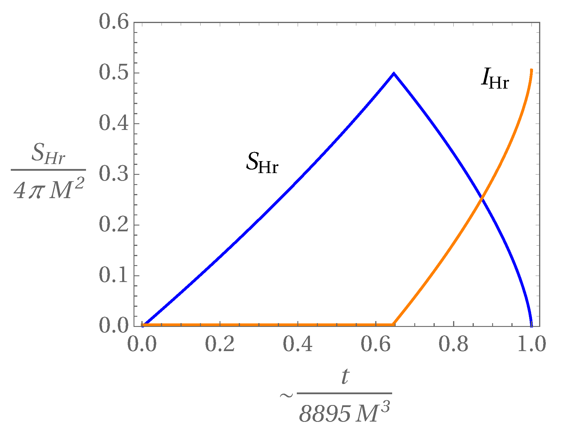
In addition, he also described, through what is today known as the Page curve (a recent nice review can be found in [
45]), the way entropy will evolve
7 (see
Figure 3) while the black hole evaporates. More recently, he has numerically estimated, based on his previous works, about emission rates of several types of particles, the way Hawking radiation entropy should evolve in time [
46]. It is believed that a correct quantum gravity theory should be able to show how Page curve emerges from the assumption of the outgoing radiation and black hole quantum states unitary evolution.
It seems pertinent to explore what the simplified model, under analysis, allow us to say about entropy and information. More precisely, we want to estimate how Hawking radiation entropy and information evolve over time according to Equation (
56). Considering the reduced density matrices (
47), we see that to properly calculate Von Neumann entropy (
52) we have to diagonalize the matrices, i.e., compute their eigenvalues
This particular calculation is only known for a few specific cases, as for example, for a system of two coupled harmonic oscillators [
47], unfortunately a distinct situation from the case studied here, namely the coupling between harmonic and inverted oscillators. Solving the eigenvalues problem allows a great simplification and the evaluation of Von Neumann entropy becomes simply
However, considering the eigenvalues problem technical difficulty, instead of computing the Von Neumann entropy we can estimate the Wehrl entropy [
48,
49],
where
is the Husimi function [
50]
The Husimi function is defined to access the classical phase space
representation of a quantum state, and it is obtained from a Gaussian average of the Wigner function
The Wigner function give us an rough criterion on how much a quantum state is distant from its classical limit but, unfortunately, it is not a strictly positive function and cannot be taken as a probability distribution in phase space
8. The Husimi representation (which is a Weierstrass transformation of Wigner function) enable us to define a strictly positive function and corresponds to the trace of the density matrix over the coherent states basis
, i.e.,
If we compare this last definition with Equations (
58) and (
59), we can understand Wehrl entropy as a classical estimate of the Von Neumann entropy, through the analogy
Hence, Wehrl’s entropy can be considered a measure of the classical entropy of a quantum system, and has already been used [
51] in the contexts of cosmology and black holes. We should notice that Wehrl entropy gives an upper bound to Von Neumann entropy, i.e.,
.
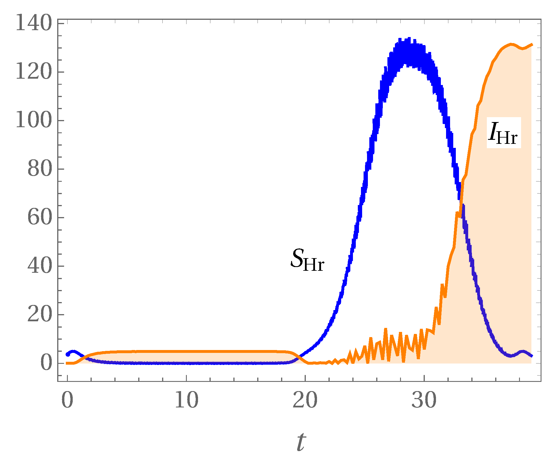
The time has come to obtain, in this simplified model, Wehrl entropy and information evolution over time for Hawking radiation. In
Figure 4 we can find the numerical estimates of Hawking radiation Wehrl entropy and information. These were obtained based on the calculation of Wigner (
Appendix B) and Husimi functions, using the reduced density matrix (
47). We can observe that the entropy start with lower values, this corresponds to a stage where entanglement and correlation between the states are weak. According to
Figure 2 this happens in a phase where the quantum states become increasingly squeezed and displaced, under the influence of the inverted potential. However when the back reaction begins to grow, correlations and degree of entanglement between the two states increase, and consequently so does the entropy, and both subsystems are forced to oscillate (counteracting the inverted potential). Finally, both states return to their initial configurations, which brings a reduction of their entropies. It is in this last phase that, with a decreasing entropy, the information contained in the state describing Hawking radiation increases as expected from the Page curve.
At this point, we can ask ourselves: how much the estimate of the
give us an accurate description of the real behaviour of the Von Neumann entropy
? Since Wehrl entropy satisfies
, inspection of
Figure 2 tell us that the variation from a lower values of the entropy (initial stage of the time evolution) to higher (intermediate stage of the time evolution) and again to lower values (final stage of the time evolution) seems to indicate, with reasonable chance, that Von Neumann entropy can present a behaviour relatively close to Wehrl entropy. In addition, the fact that we have considered the unitary evolution of the pure state
, implies that the system matrix density remains a pure state
, while the reduced density matrices, for the two subsystems, correspond to mixed states
.
7. Conclusions
Even though the simplified model, discussed in this paper, was based on modest assumptions (namely about the initial black hole quantum state, among others), it provides a simple mechanism where one can appreciate the temporal evolution of entropy and the behaviour of information (in a classical approach with Wehrl entropy being evaluated). The model has the advantage that it can be treated analytically and show how the coupling of a harmonic and inverted oscillators can produce results suggesting how the Page curve can emerge.
There are certainly many ways in which this model can become more realistic. However, it would also certainly no longer be able to be treated analytically, which would inevitably deprive it of its pedagogical appeal. In one hand, questions such as,
how the squeezing parameter evolves in this model?
what is the exact behaviour, in this model, of Von Neumann entropy ?
which aspects of the discussed estimates would benefit by considering a more realistic model?
how to apply the same procedure to the functional Schrödinger type of Equation (
19)?
can be pursued as possible future topics of investigation. On the other hand, one can also try to understand to which extent entropy, and Hawking radiation information, estimates can be made in gravitational back reaction scenarios such as those proposed in [
52,
53]. In that proposal, it is assumed that particles moving at high speeds to and from the event horizon cause a drag [
14] which has gravitational effects that can be described by the Aechelburg-Sexl metric [
54,
55]. It is worth to mention that the discussion of back reaction effects of the Hawking radiation and the correct way to derive the Page curve has been an active field of research in connection with the black hole information paradox. The reader can find complete reviews of the problem and recent progresses in that direction in [
56,
57,
58,
59] Finally, the black hole evaporation subject and the fate of the information enclosed inside it, are crucial aspects that any quantum gravity theory candidate will have to unveil. At a time when the first direct evidences of objects that in everything resemble what in General Relativity is described as a black hole are emerging, our scepticism about their real existence starts to fade away. However, it has been a long time since the conceptual problems associated with these hypothetical strange objects have challenged the limits of theoretical physics.


