Figure 1.
The error in
is plotted vs. β
cm for |η| = 0, = 1, = 3, in
Figure 1a–c, respectively. The black solid (η < 0) and red dotted (η > 0) lines define the boundary of the error depending on the value of β and η, including its sign. The blue dashed line is the average error of both η cases as a function of β. The error is relatively small for small |η| and grows with increasing |η| but does not increase significantly beyond |η| ≥ 3 because the tanh(η) → ± 1 for large |η|. Note that “1” on the vertical scale indicates 100% error. The data errors are constrained between the red dotted and solid black lines from this effect.
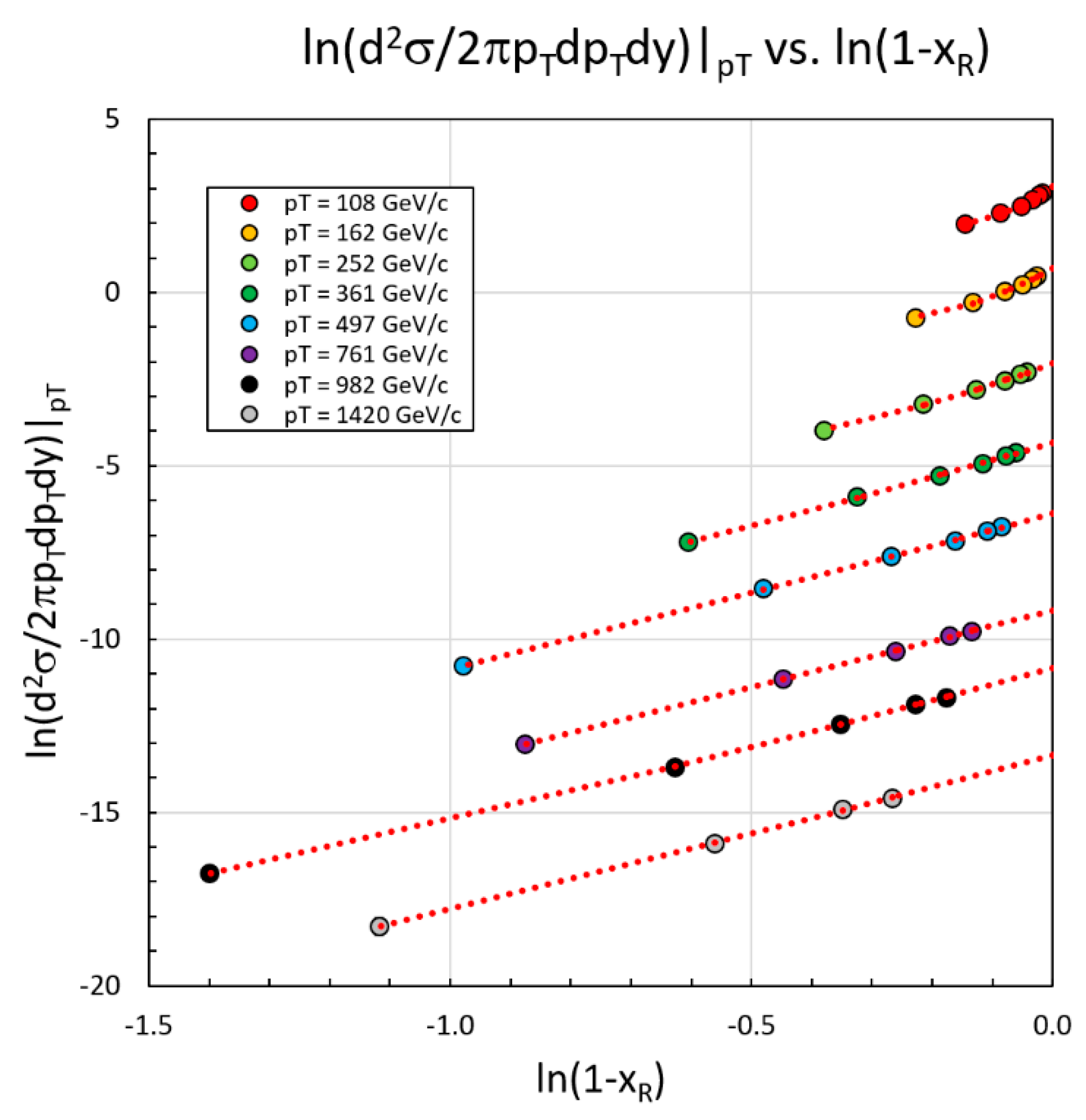
Figure 2.
Demonstration of the ansatz of Equation (3) for some selected values of in GeV/c for inclusive jets defined by the anti-kT algorithm, with R = 0.4 measured by the ATLAS collaboration at = 13 TeV. The plot demonstrates that the log of the invariant cross section at constant is a quadratic in ln(1 – ). The error bars are smaller than the data points. The red dotted lines indicate minimum χ2 fits to Equation (3). The extrapolation to ln(1 – ) = 0 ( = 0) determines . The right-most point of each constant line corresponds to y = 0 and the gap between this point and right-hand axis is the region beyond the kinematic boundary for given value of and . For the ensemble of fits at constant , the χ2/d.f. = 14 for 79 degrees of freedom (p = 1.0).
Figure 3.
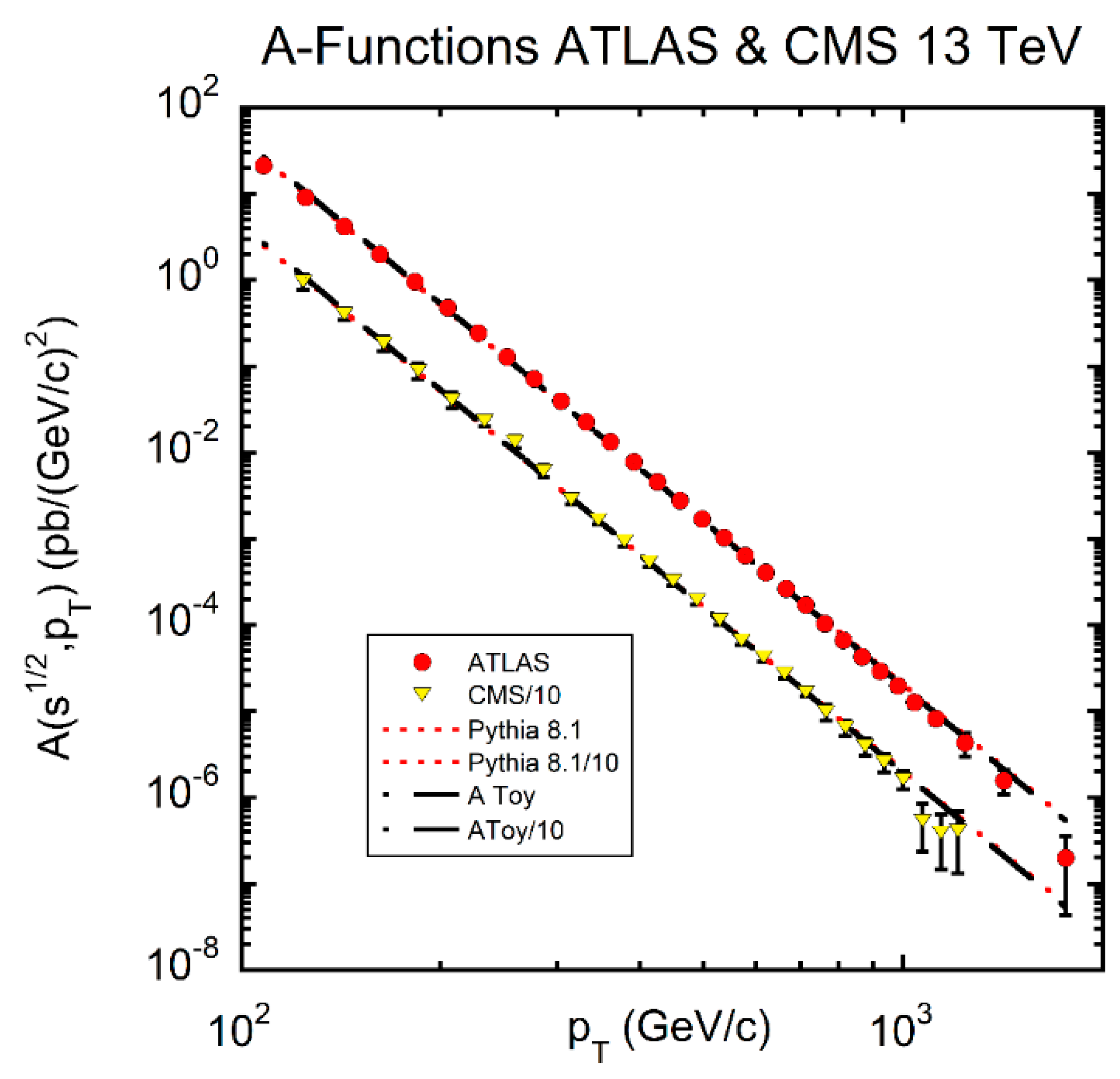
The a function dependence for a 13 TeV inclusive jet cross section (R = 0.4) measured by ATLAS (red circles) and CMS (yellow triangles) divided by 10. All data point errors—statistical and systematic—were added in quadrature. The dashed black lines represent power law fits of the Toy MC. The Pythia 8.1 simulations are indicated by the red dotted lines. Both simulations were normalized to data. The MC representations of the data are indistinguishable on this plot. The respective power law fits for 29 degrees of freedom (d.f.) for ATLAS are: fitting the data to a power law χ2/d.f. = 1.13, (p = 0.288), Pythia 8.1 power law fit to data χ2/d.f. = 1.24 (p = 0.18) and Toy power law fit to data χ2/d.f. = 1.13 (p = 0.288). For CMS 25 d.f. the fit qualities are χ2/d.f. = 0.60 (p = 0.94), 0.76 (p = 0.80) and 0.66 (p = 0.90), for data, Pythia 8.1 and Toy, respectively. The parameter in Equation (5) was set to 0.
Figure 4.
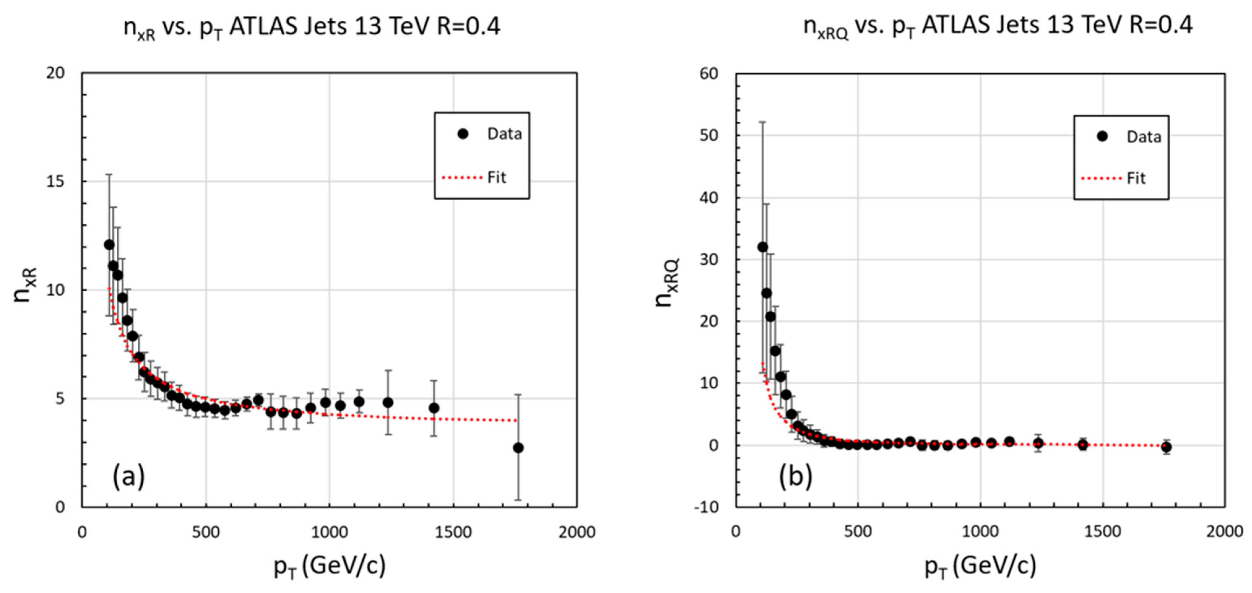
The power indices (a) and (b) are plotted as a function of . The red dotted curves are the result of minimum χ2 fits to Equation (10). We find D = (7.0 ± 1.1) × 102 GeV/c, = 3.6 ± 0.2 with χ2 = 14 for 29 degrees of freedom (p = 0.99) and DQ = (1.5 ± 0.4) × 105 (GeV/c)2 and = 0.06 ± 0.1 with χ2 = 24 for 29 degrees of freedom (p = 0.73). While the fits have good χ2 values, they systematically underestimate the values of and for ≤ 200 GeV/c.
Figure 5.
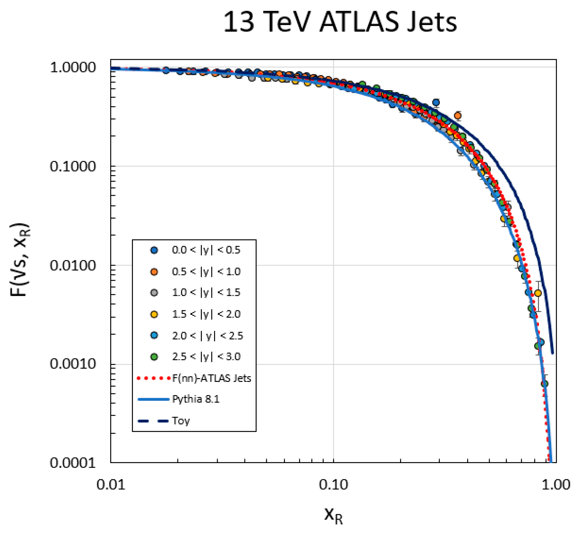
The for 13 TeV inclusive jets (R = 0.4) is plotted as a function of for various slices of <|y|> indicated by the numbers in the legend. Note that all the data points at different y values fall on the same line and that the red dotted line represents Equation (14). The error bars represent the systematic and statistical errors added in quadrature. The fit of data by Equation (14) has a χ2/d.f. = 1.06 for 170 degrees of freedom (p = 0.28). The solid blue line represents Pythia 8.1 simulation (χ2/d.f. = 3.5, p ~ 0)) and the black line the prediction of the Toy MC (χ2/d.f. = 36.6 p ~ 0).
Figure 6.
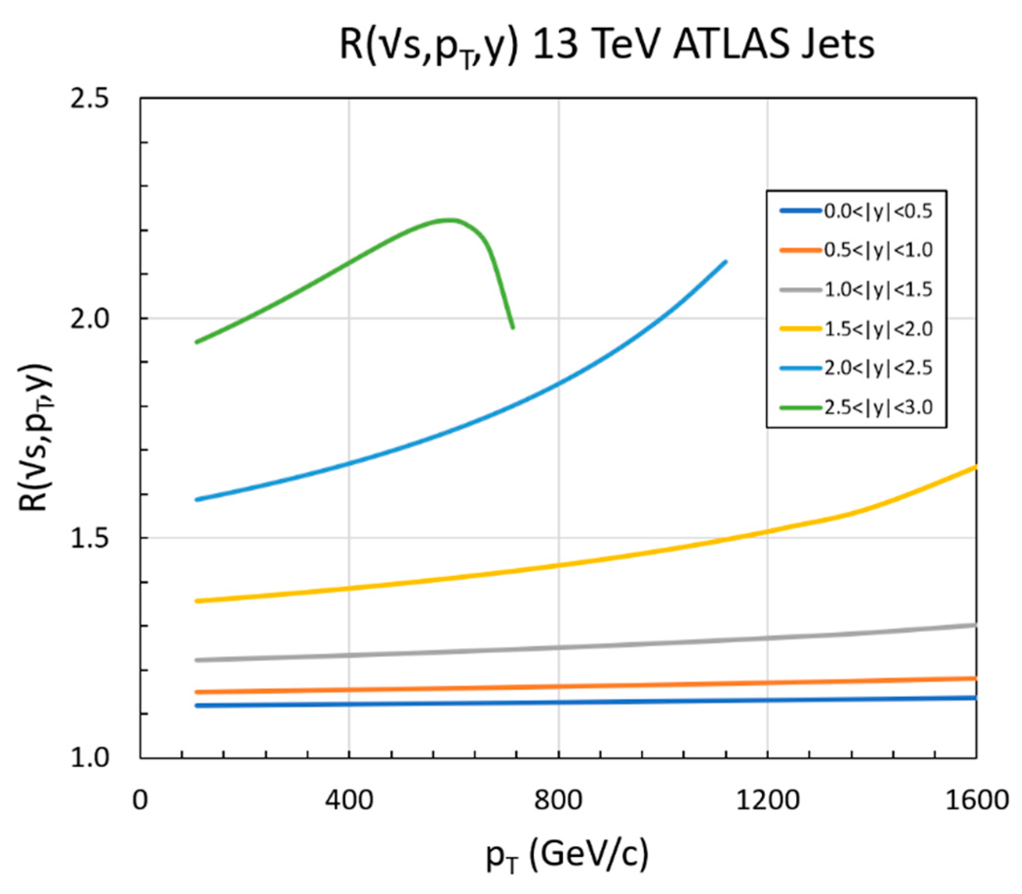
The correction function for 13 TeV inclusive jets determined by the measured values of D and DQ is plotted as a function of for various values of |y| given by Equation (13).
Figure 6.
The correction function for 13 TeV inclusive jets determined by the measured values of D and DQ is plotted as a function of for various values of |y| given by Equation (13).
Figure 7.
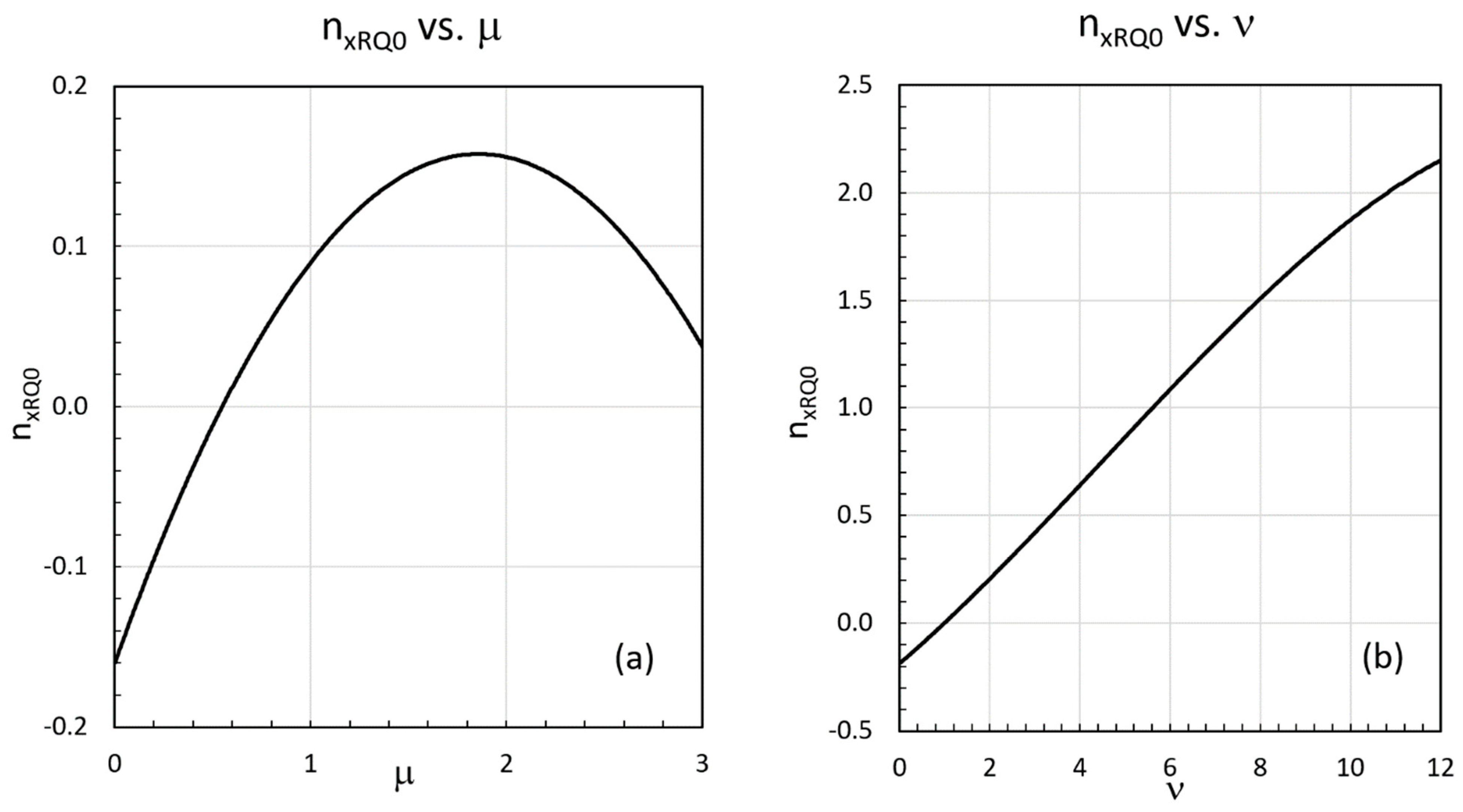
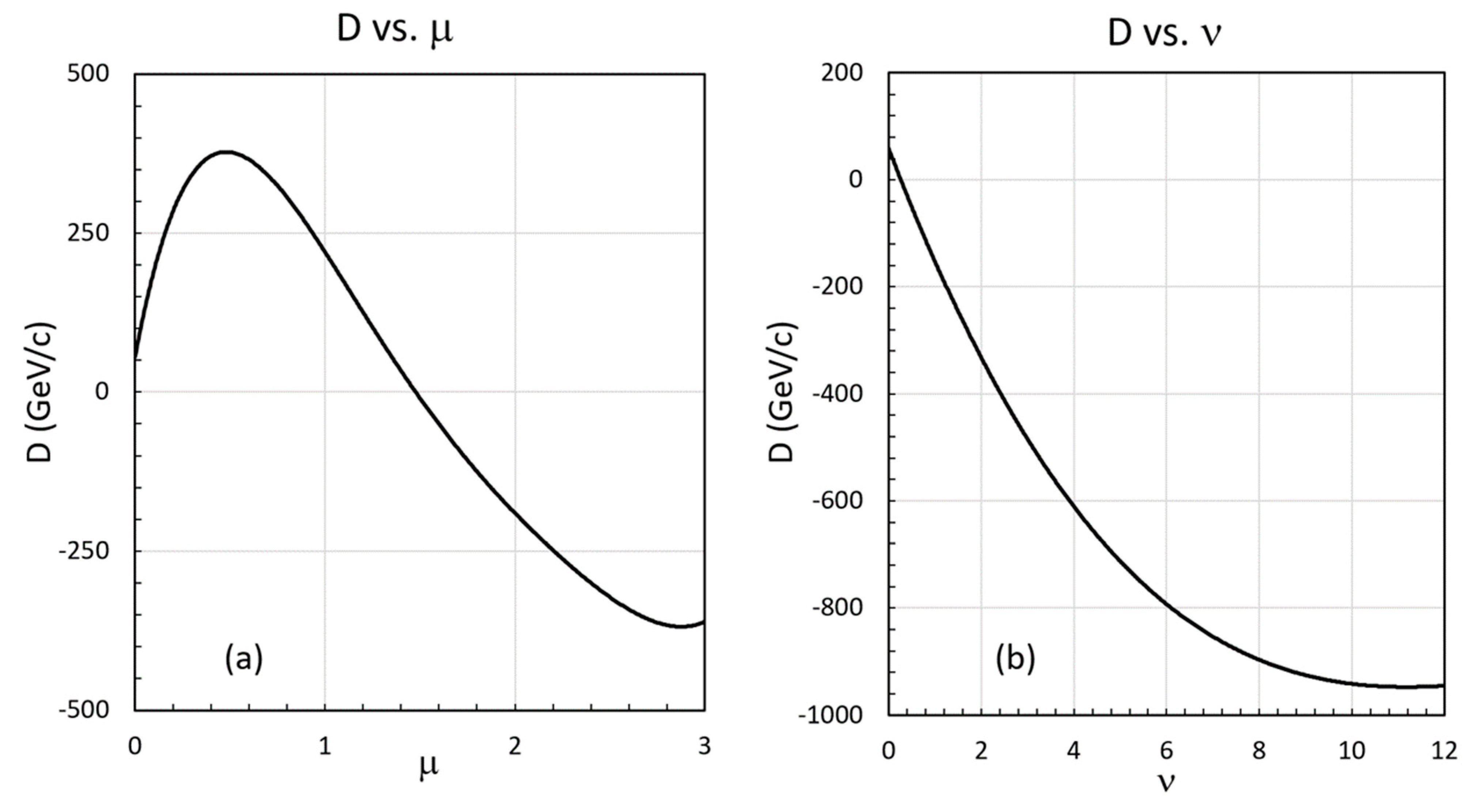
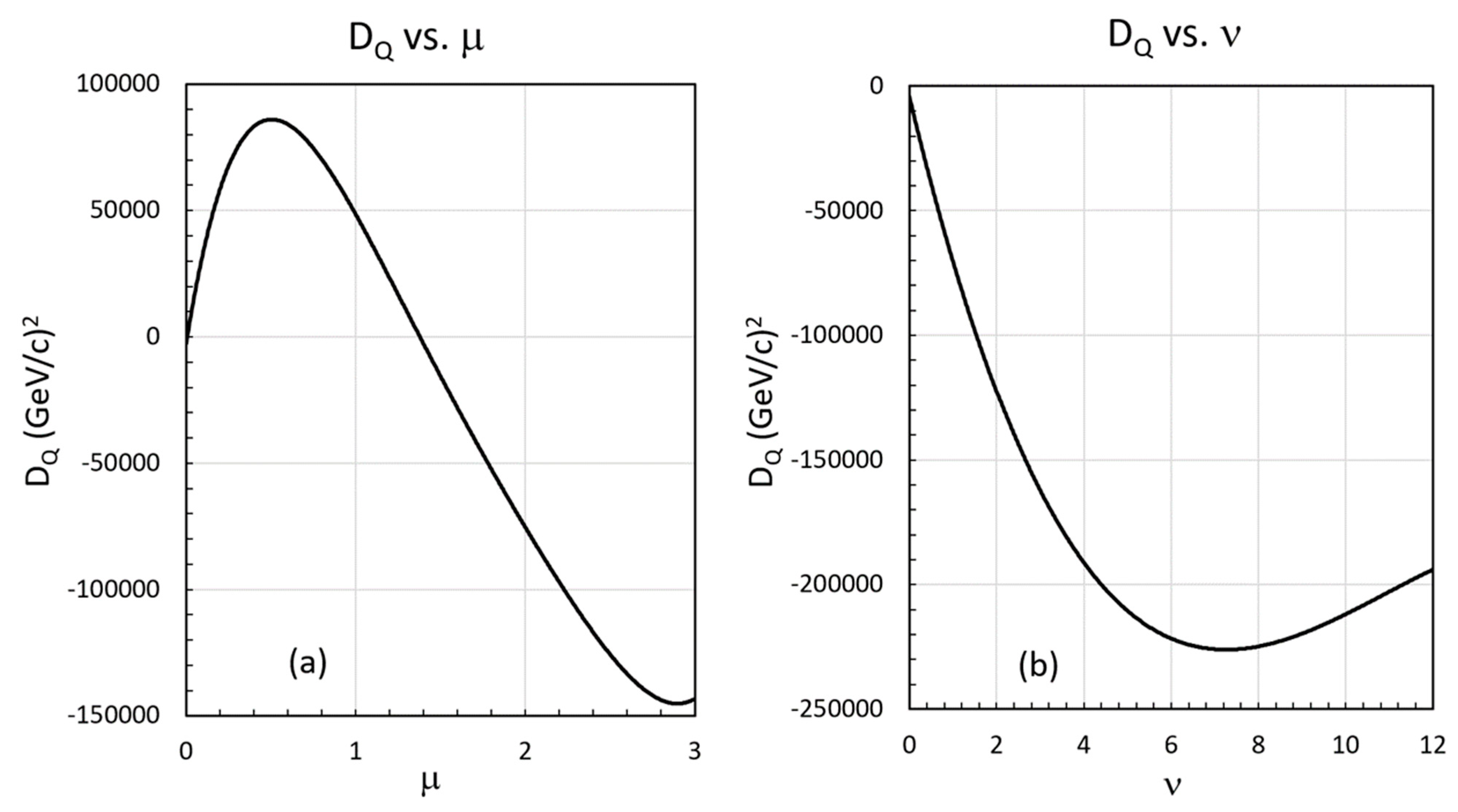
Shown are the values of the toy inclusive jet simulations as a function of the power indices μ and ν of our two simple models of the gluon PDF. The sensitivity of to μ, the power of (1/x)μ is shown in (a). The black dotted line indicates the value resulting from the Pomeron and the red solid line and horizontal error bars indicate the central value of of the ATLAS 13 TeV inclusive jet data and errors, respectively. The sensitivity of to the power index ν of (1 − x)ν is shown in (b). The red lines indicate the experimental value from the ATLAS jet data with error bars. Notice that the power index of the a function is mostly controlled by the low x-peaking behavior of the PDF shown in (a), whereas the behavior is controlled by the parameter ν that shapes the high-x behavior shown in (b).
Figure 8.
The resultant F-functions in the two cases are shown. For (a), the red through green lines represent the functions for μ = 0, 0.5, 1, 2, respectively, and the Pomeron is shown by the dotted black line. In (b), we show the F-functions for ν = 0 (red line), 1, 3, 6 and 9 (black line). ATLAS data lie between the yellow and green lines in (b). The F-functions were calculated from their respective and values for each μ and ν.
Figure 9.
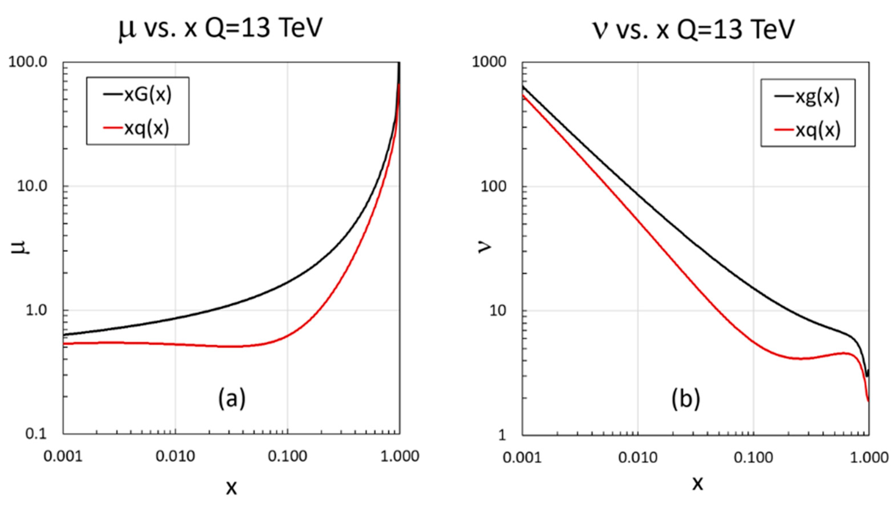
The effective
μ (
a) and
ν values (
b) for the CT10 gluon (black lines) and quark (red lines) PDFs at
= 13 TeV. Notice that
μ for quarks is smaller than that for gluons implying that
for quark scattering is smaller than the corresponding values for gluons—consistent with the discussion above. Further, we note that since the quark distribution dominates at high x, the value of
is largely determined by the quark PDFs at x > 0.1 where there is a ‘valence shelf’ ν ~ 4 consistent with the
value measured in jets (ATLAS
= 3.6 ± 0.2) by the
– ν relation of
Figure 7b. Therefore, our analysis using
and
sheds light on the shape of the PDFs in different regions by the different sensitivities of the parameters
,
D,
DQ,
and
and are nicely correlated with the shapes of the colliding PDFs.
Figure 10.
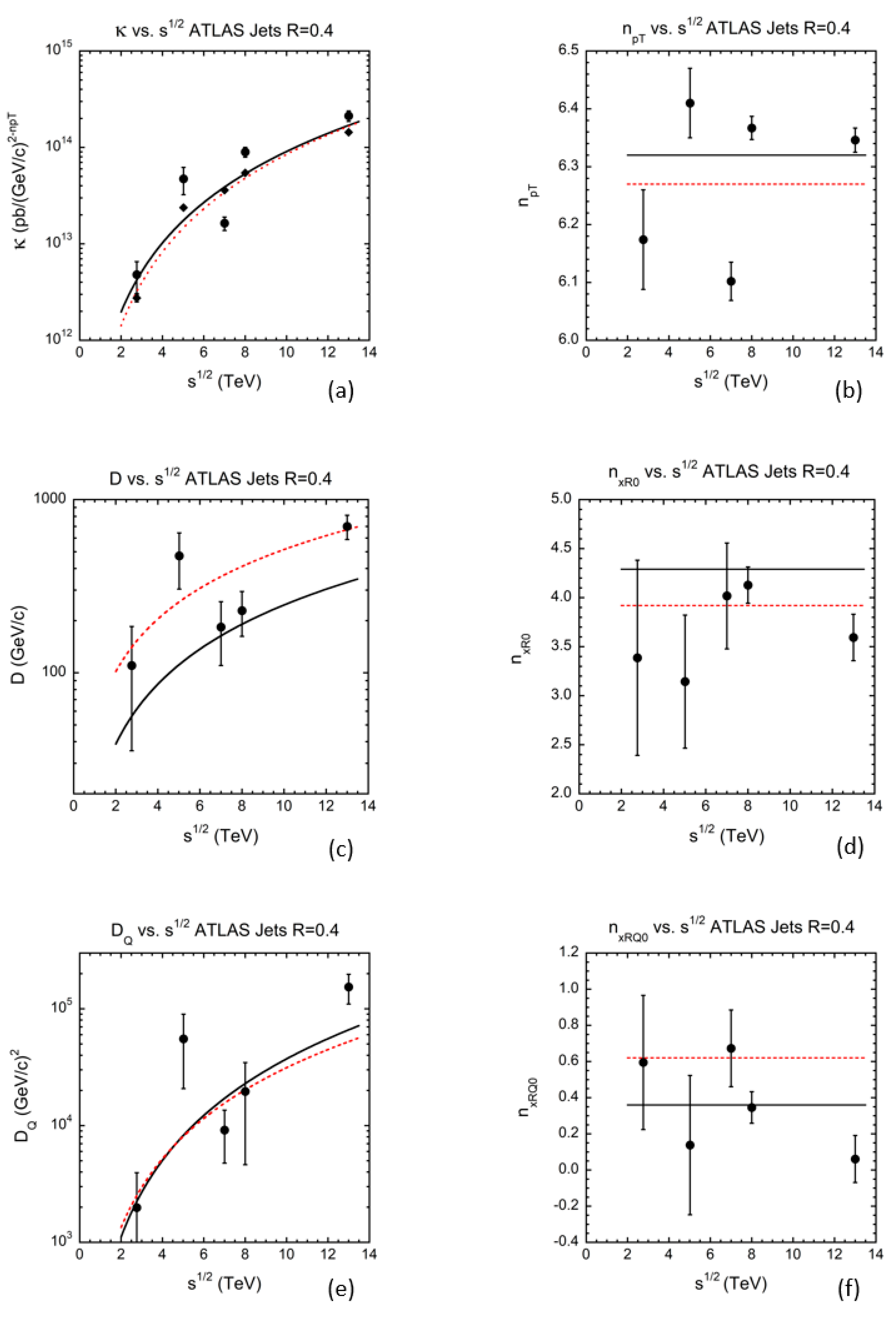
The fit values for each of the inclusive jet measurements performed by the ATLAS collaboration are plotted as a function of . The red dotted lines are power law fits ((a) κ(), (c) D(s), (e) DQ(s), respectively) to the toy model MC described in the text and the solid black lines are the corresponding power law fits of the Pythia 8.1 simulations. The power indices are plotted in (b) , (d) , (f) , respectively. The simulations show little s dependence, so only the average power indices are shown. Since the power index, , shows no systematic dependence, we show the κ values computed by fixing to its average. Those points are shown as diamonds in (a).
Figure 11.
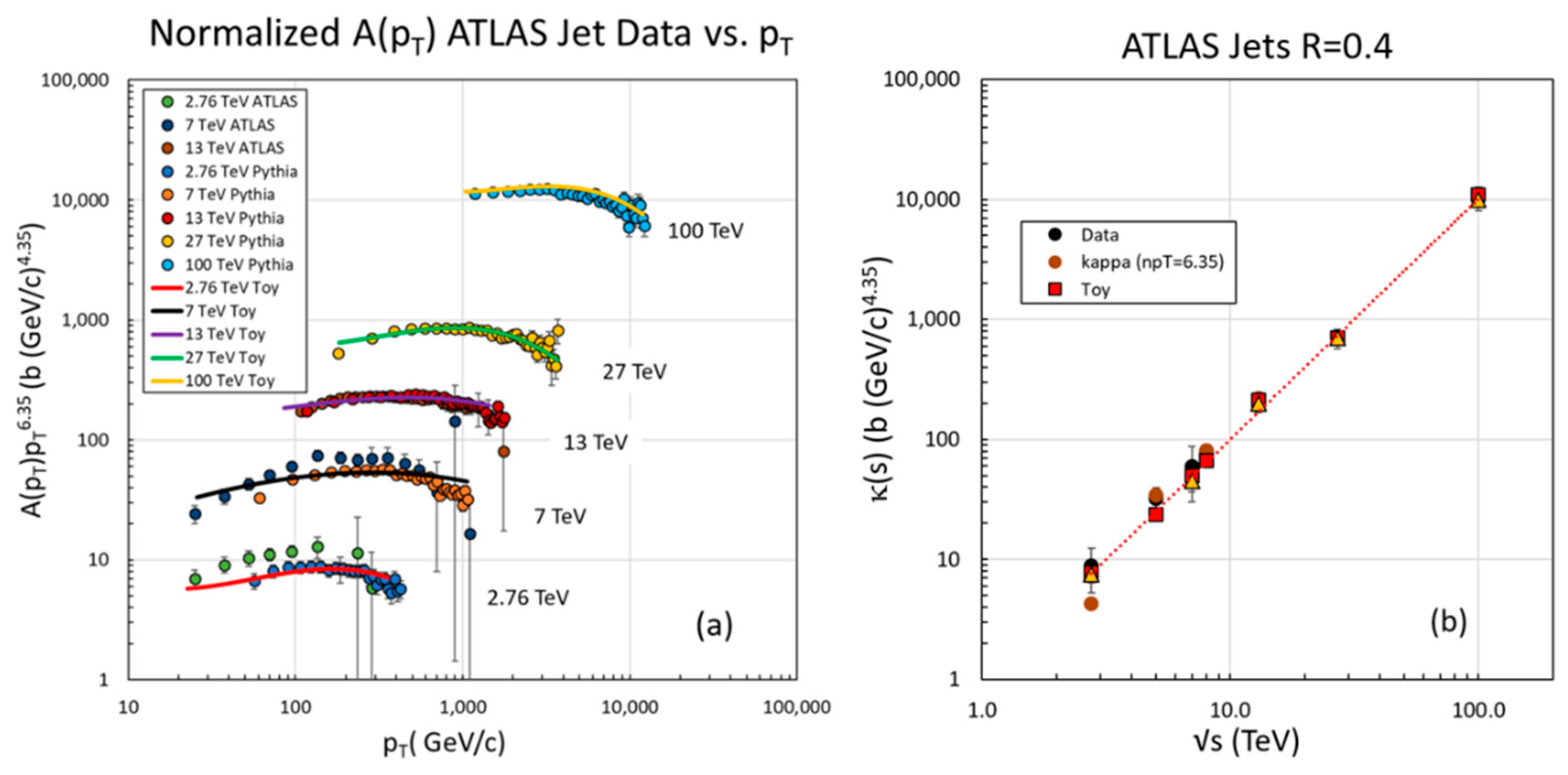
(a) The functions multiplied by 6.35 for ATLAS inclusive jet data (R = 0.4) are plotted vs. . The Toy MC simulations for each energy are displayed by the red dotted lines and the Pythia 8.1 simulations are indicated by the circles with black outlines. The Toy MC has been smoothed by a cubic polynomial fit in . It follows Pythia 8.1 for the three overlapping values, but both tend to underestimate the data at 2.76 (green circles) and 7 TeV (blue circles). All three functions overlap at = 13 TeV, where the simulations were normalized. The vertical axis is a measure of the magnitude parameter κ(s) in Equation (6) given in units of barns (GeV/c)4.35. On the right, (b), κ(), computed by the average of each normalized is plotted as a function of for data and the two MC simulations. The errors of the averaged are the standard deviation about the averages. Also shown is the value of κ() of data computed by fixing = 6.35. The red dotted line is a fit to the Pythia 8.1 simulation consistent with κ() ~ ()2. Note that each normalized a function is not a constant indicating a violation of the pure power law.
![Universe 07 00196 g011 Universe 07 00196 g011]()
Figure 12.
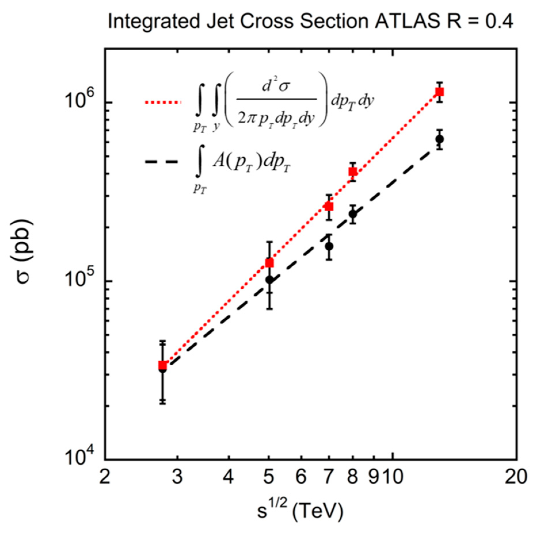
The integrated jet cross section for 100 ≤ ≤ 3000 GeV/c, ≤ 0.9, and |y| ≤ 3.0 for the parameterization of the inclusive cross section as measured by ATLAS (red squares) and of the integral of the corresponding a functions (black circles). The error bars were estimated from the relative errors of κ(s), the a function magnitude parameter. The red dotted line and dashed black line represent a power law growth ()2.29 ± 0.05 and ()1.89 ± 0.09 with χ2/d.f. of 1.3/5 (p = 0.93) and 0.62/5 (p = 0.99), respectively. The integrated cross section grows faster in than the integrated a function because of the broadening of the rapidity distribution with increasing .
Figure 13.
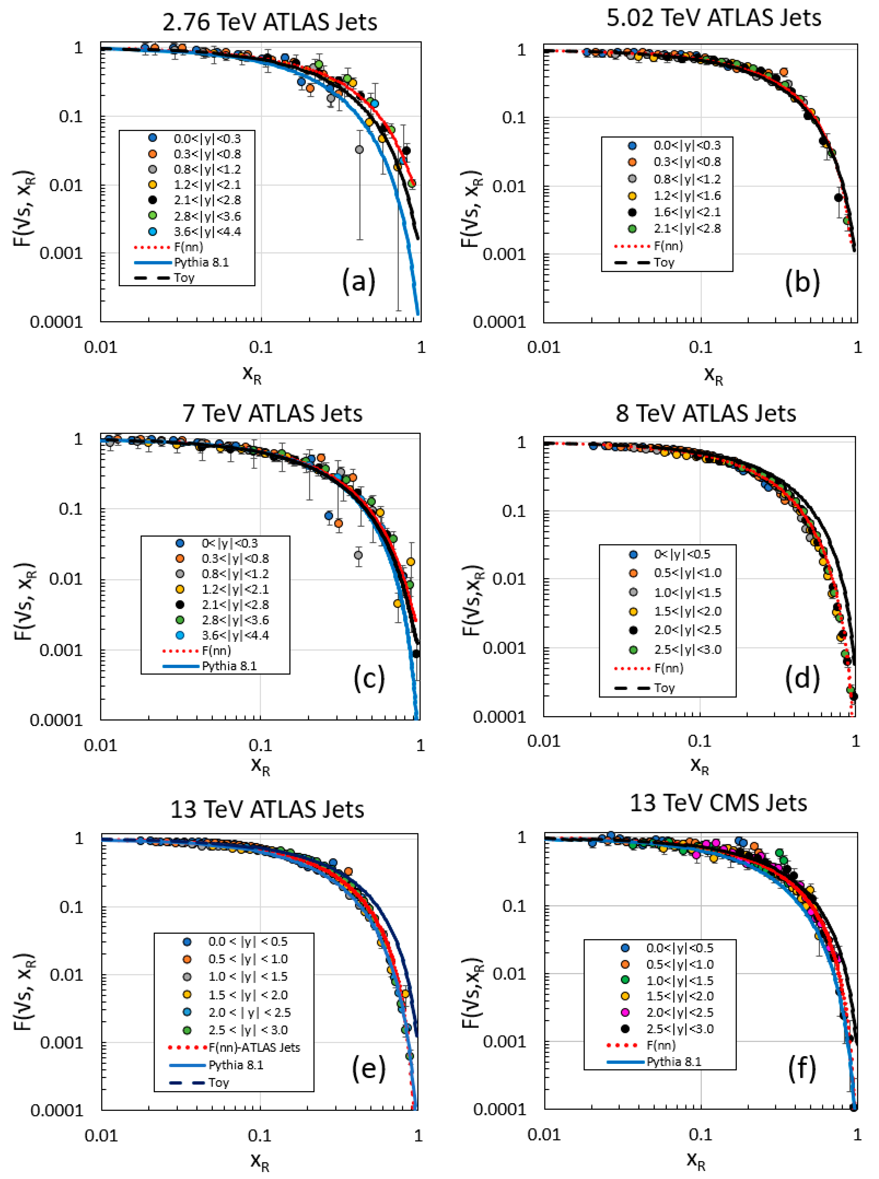
The distributions for five values of for ATLAS inclusive jets ((a–e) for = 2.76, 5.02, 7, 8, 13 TeV, respectively) and for CMS jets at 13 TeV—(f). The red dotted line represents a fit to the data (Equation (16)), the solid blue line the results of a Pythia 8.1 simulation and the dashed black line the results of the toy model simulation. Pythia agrees roughly with data for 7 and 13 TeV but underestimates the data at 2.76 TeV. The Toy model generally overestimates data at high for 8 and 13 TeV.
Figure 14.
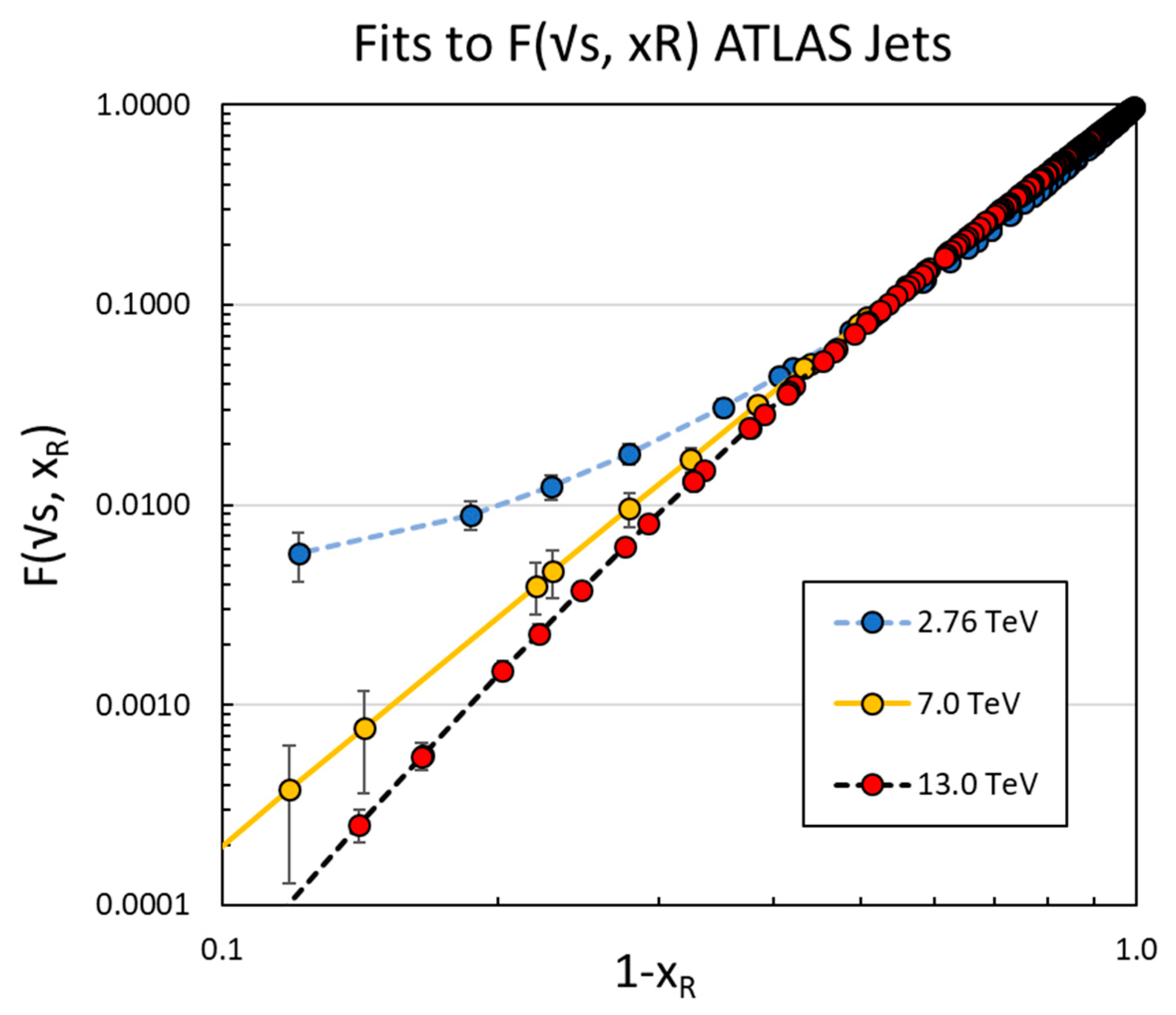
Shown are the fits to Equation (16) of the F-function of ATLAS inclusive jet data (R = 0.4) taken at 2.76, 7 and 13 TeV indicated by the blue dotted, solid gold and dashed black lines, respectively. The ‘data’ points plotted are the values of the fit with the error bars indicating the error of the fit plotted at the same (1 − ) values of the data. The plot shows that the data follow a power law ~ (1 − )nxR0 for low , but deviate significantly at higher —especially for at 2.76 TeV. The deviation is controlled by the term. Some s dependence is expected since the gluon, quark and antiquark contents of the proton evolve with .
Figure 15.
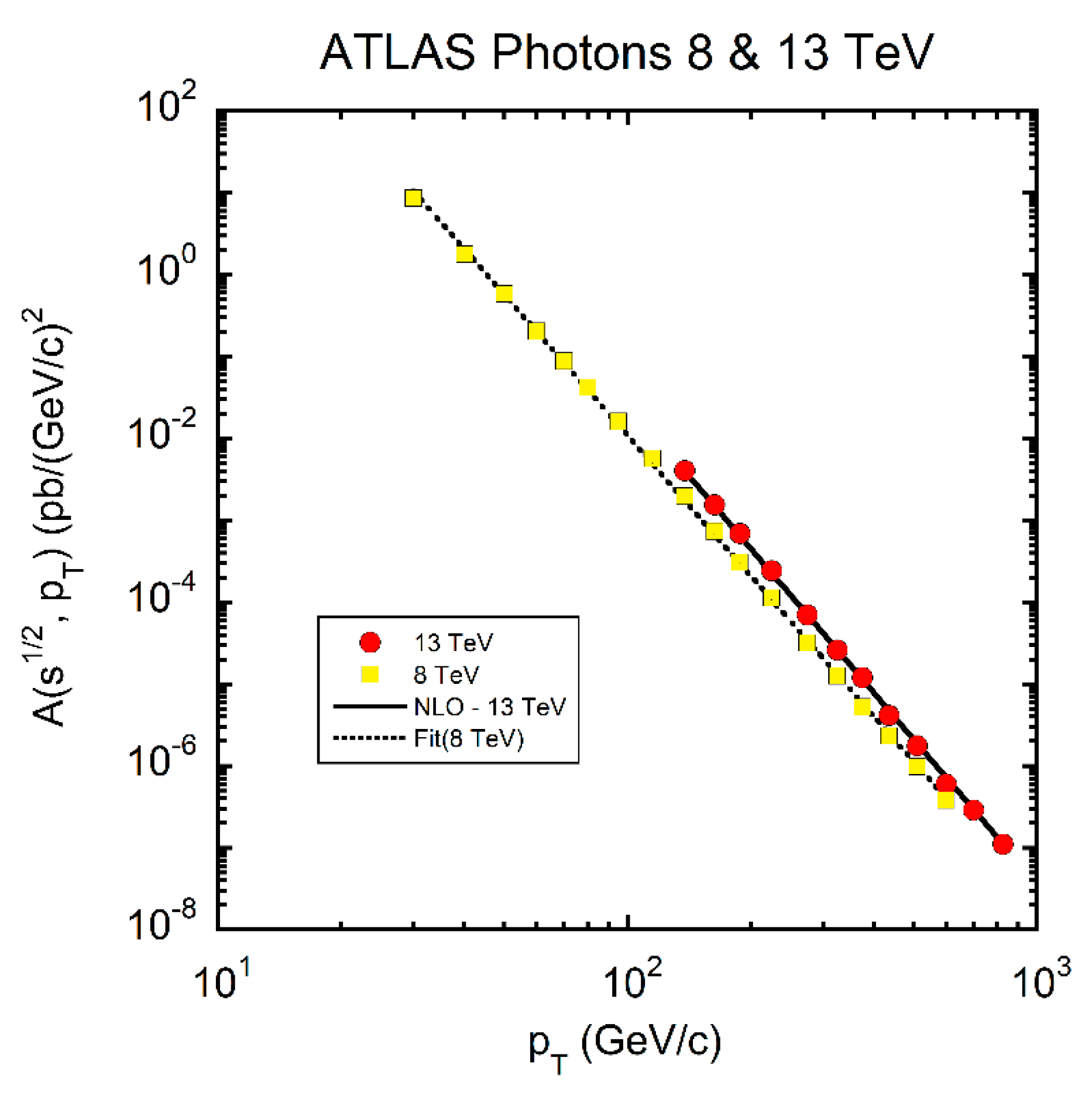
The functions for direct photons measured in the ATLAS detector for = 8 TeV (yellow squares) and = 13 TeV (red circles). The dotted line is a power law fit to the 8 TeV data and the solid black line is a fit to the NLO simulation for the 13 TeV data with parameters κ = (1.28 ± 0.95) × 1010 pb/(GeV/c)2-npT and = 5.85 ± 0.12.
Figure 16.
The power indices
and
((
a,
b) respectively) for inclusive isolated photons measured in the ATLAS detector for
= 13 TeV compared to simulations. The red dotted lines represent the results of our Toy model simulation and the solid black lines the theory simulation shown in the ATLAS paper [
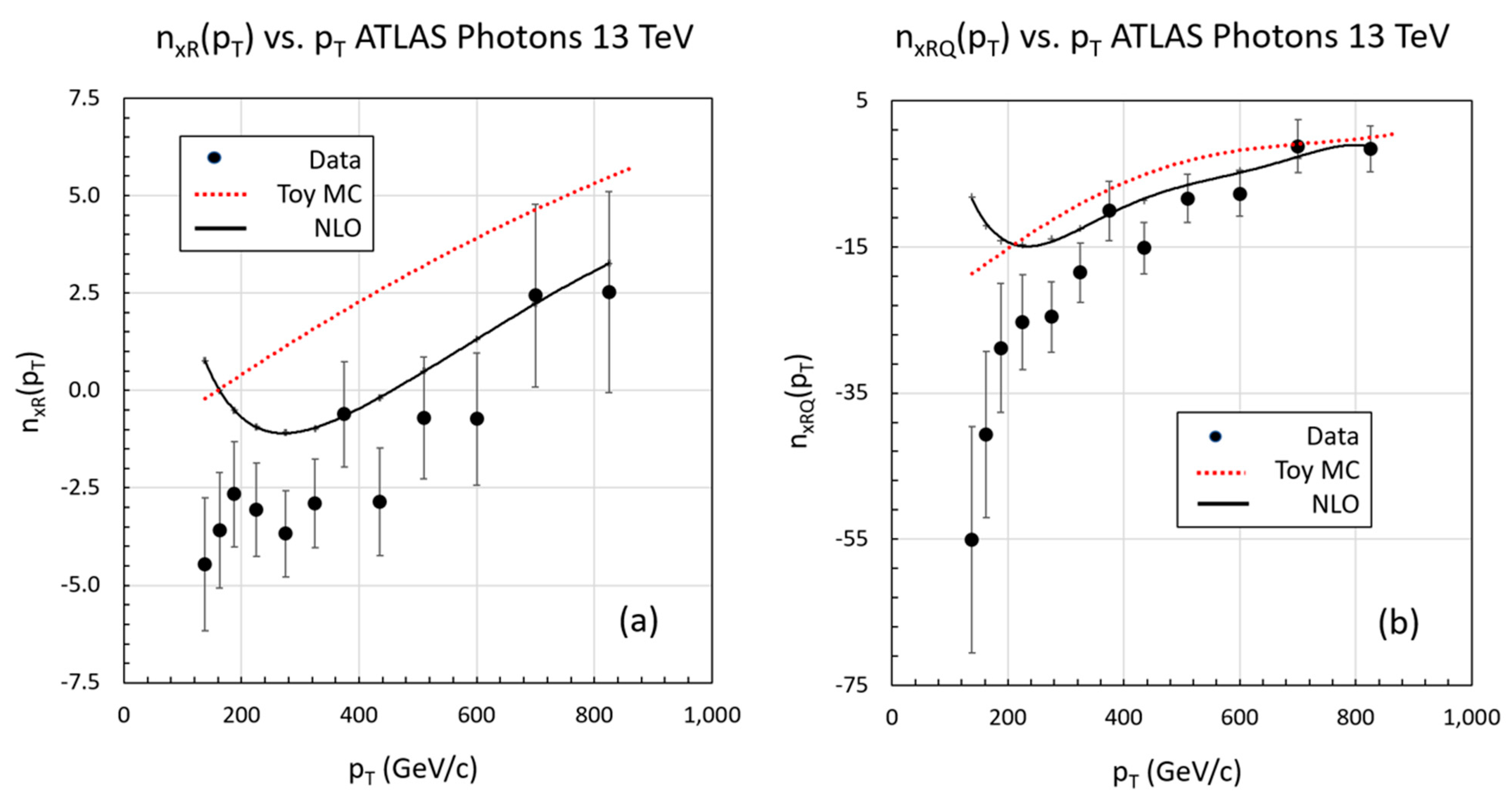
37]. Both the Toy MC and NLO simulation tend to overestimate the power indices. The NLO simulation is a better representation of
but is approximately the same quality as the Toy MC for
. The large systematic errors of the NLO simulation are not shown.
Figure 17.
The ratio of the inclusive isolated photon cross sections measured by the ATLAS collaboration at = 8 and 13 TeV is plotted as a function of (ET) for various slices of |η| in (a–d). The dashed black curves represent the NLO QCD calculation and the red dotted curves are the results of our Toy MC simulation. The NLO calculation is a better representation of the data but it is noteworthy that the Toy simulation is so close to the data—especially at the two larger |η| bins. This is an indication that most of the dependence is due to the decrease in the cross section as → 1, the high kinematic boundary.
Figure 18.
Shown is the transverse momentum
and modified transverse momentum
dependences of the a function for B
± production at 7 TeV (LHCb [
45]). It is evident that the transverse momentum distribution
indicated by the yellow circles can be corrected by the empirical mass term
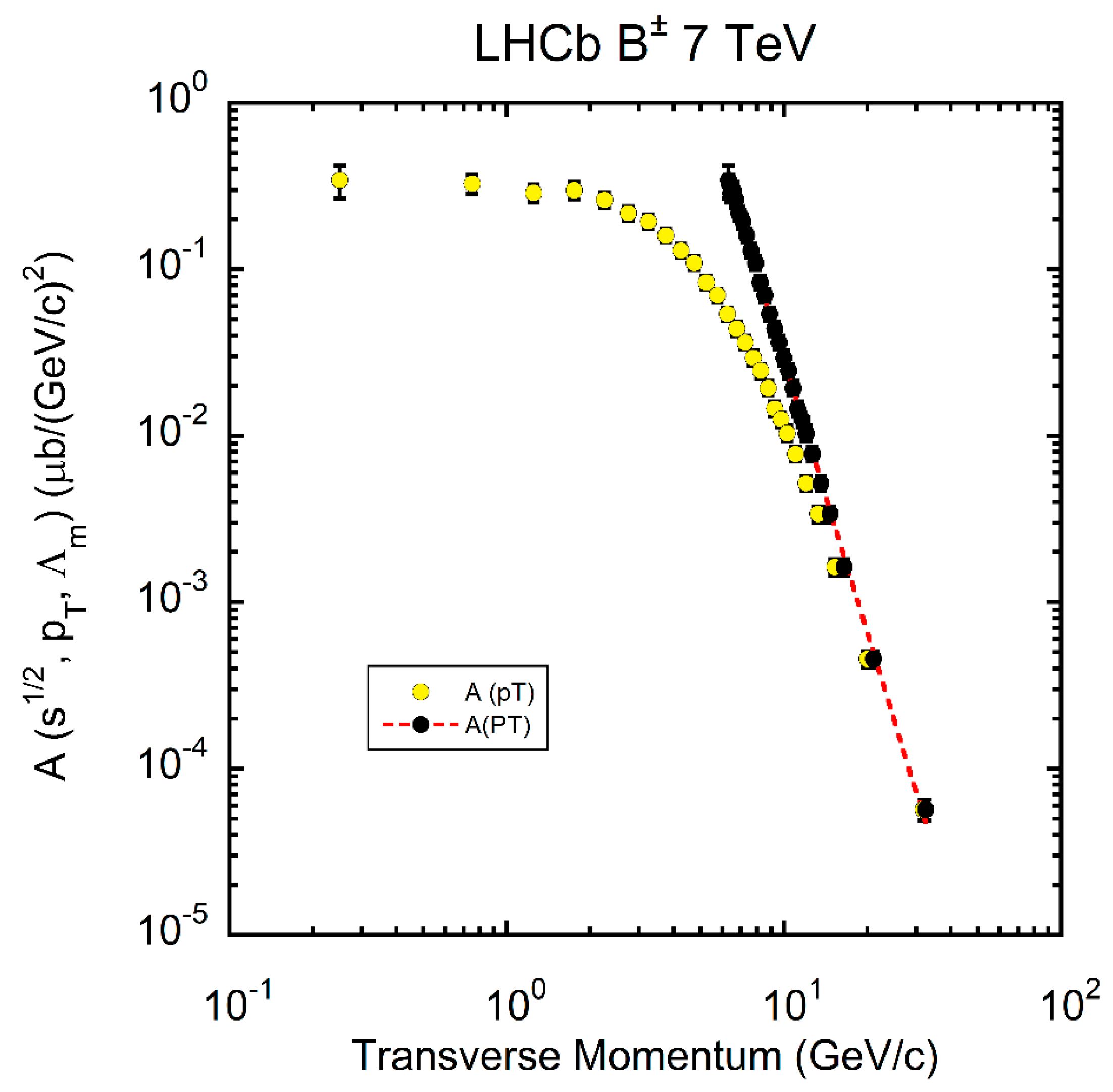
= 6.3 ± 0.3 GeV/c to reveal the underlying power law indicated by the black circles as given in Equation (3). The power index of the
distribution is
= 5.5 ± 0.2, smaller than that of the inclusive (u-d-s-g) jet production cross sections shown in
Figure 3. The 3-parameter fit determines κ = (8.8 ± 4.7) × 10
3 μb (GeV/c)
npT−2 with χ
2/d.f. = 6.6/24 (
p = 1.0).
Figure 19.
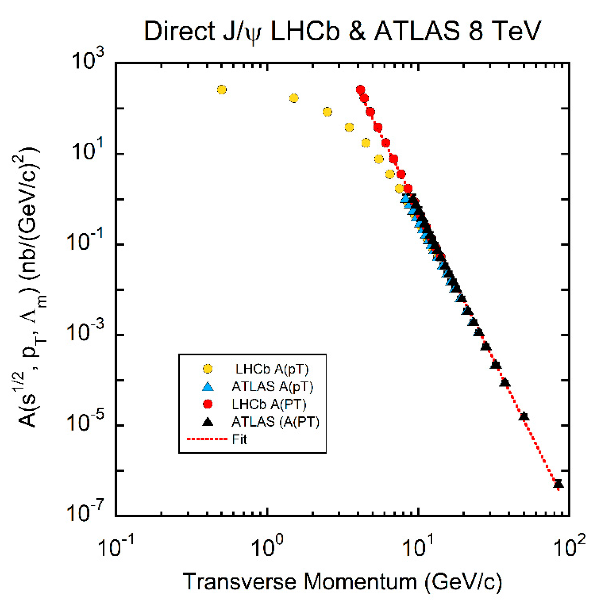
The values for J/ψ prompt mesons as a function of transverse momentum are plotted for both LHCb (circles) and ATLAS data (triangles) sets at = 8 TeV. Two values of the transverse momentum are plotted for each point—the value and the modified transverse momentum value derived from given by . The yellow circles and blue triangles (mostly covered by black triangles) are versus for the LHCb and ATLAS data, respectively, and the red circles (LHCb) and black triangles (ATLAS) are the same data plotted versus the modified transverse momentum, . Note that all data have the same power index = 6.53 ± 0.03 indicated as a simultaneous fit to both data sets. The common fit value results in = 3.93 ± 0.02 GeV/c. The ATLAS data were taken in the interval 0 ≤ |y| ≤ 2.0 and the LHCb data in the non-overlapping region 2.0 ≤ |y| ≤ 4.5, thereby demonstrating the independence on |y| of as a function of .
![Universe 07 00196 g019 Universe 07 00196 g019]()
Figure 20.
Shown in (a) is the transverse mass parameter as a function of the single particle mass in single particle inclusive production as illustrated in the fit for B± shown above. The red dotted line represents a fit to the data, not including the Υ(nS) data resulting in = (1.17 ± 0.04) m + (0.40 ± 0.04) where is in momentum units (GeV/c) and m is in mass units (GeV/c2). The photon point, where m = 0 with = 0, was not included in the fit. The LHCb Υ(nS) data are inconsistent with the general trend for lower masses suggesting that the –m relation breaks down for high mass. In (b) are the values of the corresponding fits in ascending magnitude vs. the particle species. The photon and jet points are the values of the spine fits—hence the small errors.
Figure 21.
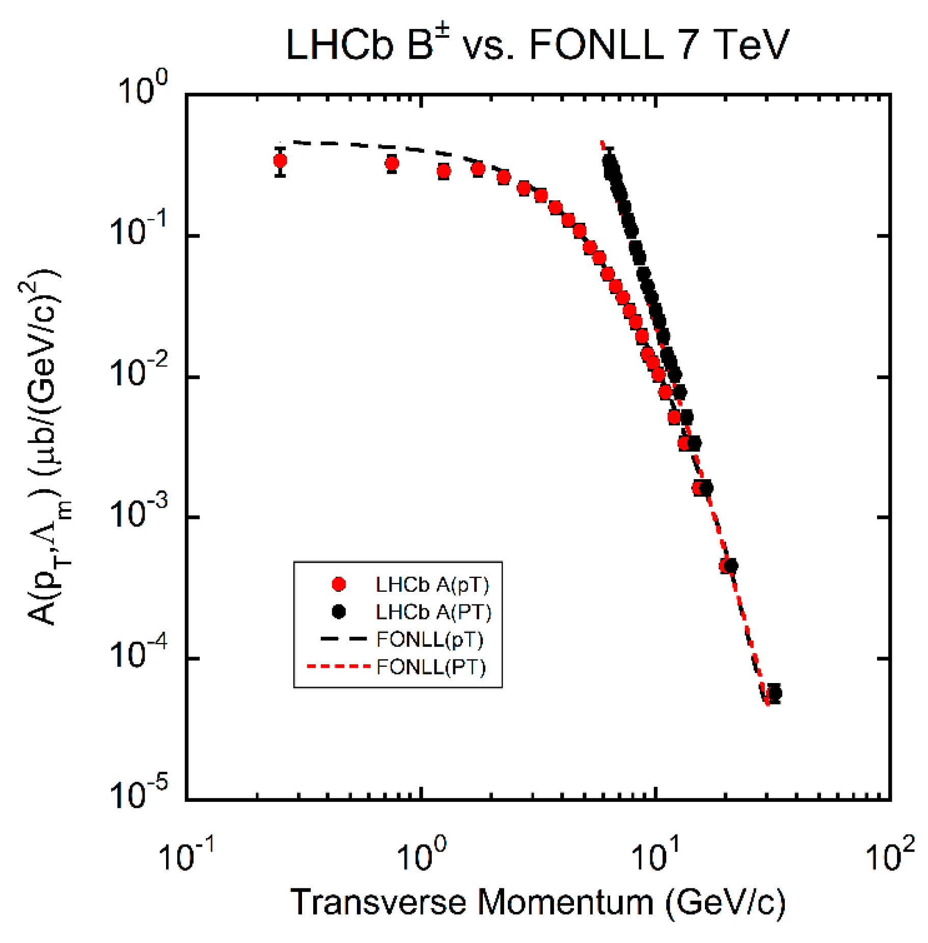
The resulting function for the FONLL simulation of inclusive production of B-mesons at = 7 TeV (orange diamonds and red dotted line) superimposed on the LHCb data (red and black circles) for MC and data plotted vs. the transverse momentum and the modified transverse momentum, . The MC is in good agreement with the data and both MC and data follow a power law in the modified transverse momentum, .
Figure 22.
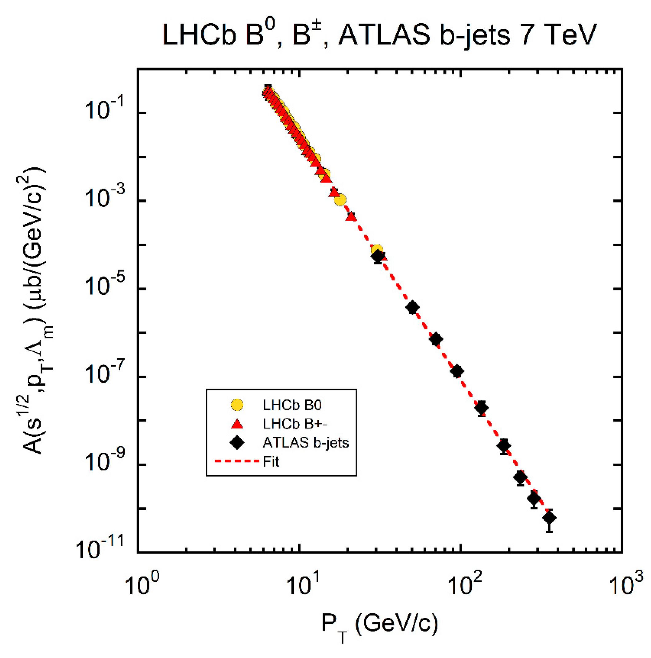
Comparison of the distributions of b-jets (black diamonds) measured in ATLAS normalized by an empirically determined multiplicative factor of 1.4 × 10⁻⁴ with LHCb B-meson data (B0 and B± shown as yellow circles and red triangles, respectively). Each data set is plotted versus the modified transverse momentum . The red dotted line is a simultaneous power law fit in the modified transverse momentum, , of all three data sets resulting in = 5.51 ± 0.03 and = 6.3 ± 0.3 GeV/c (χ2/d.f. = 14.3/52, p = 1.0).
Figure 23.
The power terms, for (1 − )nxR are plotted vs. for LHCb B± data (black points) and for the FONLL simulation (red dotted line). The errors were computed from the experimental statistical and systematic errors added in quadrature and the fitting errors in the determination of .
Figure 23.
The power terms, for (1 − )nxR are plotted vs. for LHCb B± data (black points) and for the FONLL simulation (red dotted line). The errors were computed from the experimental statistical and systematic errors added in quadrature and the fitting errors in the determination of .
Figure 24.
On the left, (a), we show the function for B± data measured at 7 TeV by the LHCb collaboration and on the right (b) the b-jet measured by ATLAS at the same . Notice that the rapidity and regions of the LHCb and ATLAS data sets are disjoint. We have plotted LHCb vs. ATLAS: 2.0 ≤ | y| ≤ 4.5 vs. 0 ≤ |y| ≤ 2.1, and 0.25 ≤ ≤ 31.75 GeV/c vs. 30 ≤ ≤ 355 GeV/c, respectively. The regions of the two functions are roughly the same, 0.008 < < 0.3. The F-functions for B± and b-jets are very different from g-u-d-s jets which are indicated by the blue dotted line in the right-hand graph.
Figure 25.
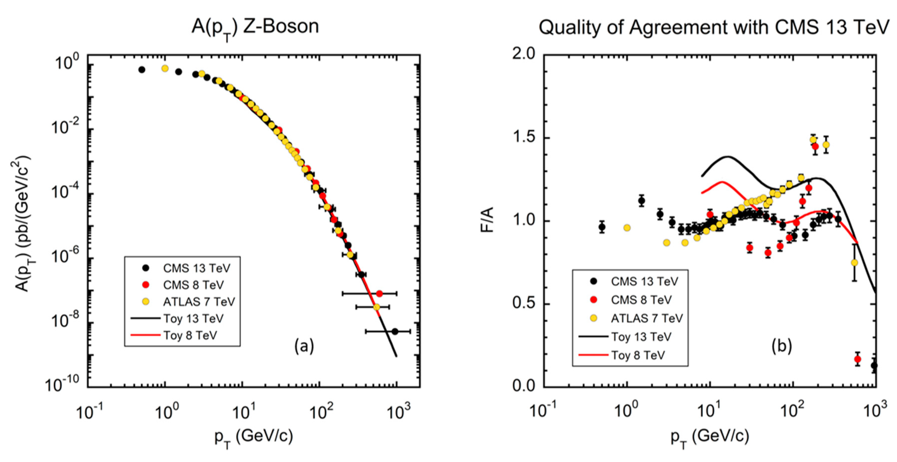
In the left plot, (a), the a function of inclusive Z-boson production measured by the CMS collaboration at 8, 13 TeV are compared with the ATLAS 7 TeV data and Toy MC simulations at 8 and 13 TeV. All data are normalized to the CMS 13 TeV data set. The bin widths have been plotted for the highest ~5 bins of the data. There are two salient features of the a functions apparent in the plots: (1) the turnover at low and (2) the emergent power law behavior at large . On the right (b) are shown the ratio of the normalized data and MC to 13 TeV CMS data set. The black circles in the right plot indicate the quality of a 4th-order log(A)-log() polynomial fit to 13 TeV data used to compare data sets. The overall agreement is within ±50% for all quality measures (fit, data-data, data-MC) except at highest points.
Figure 26.
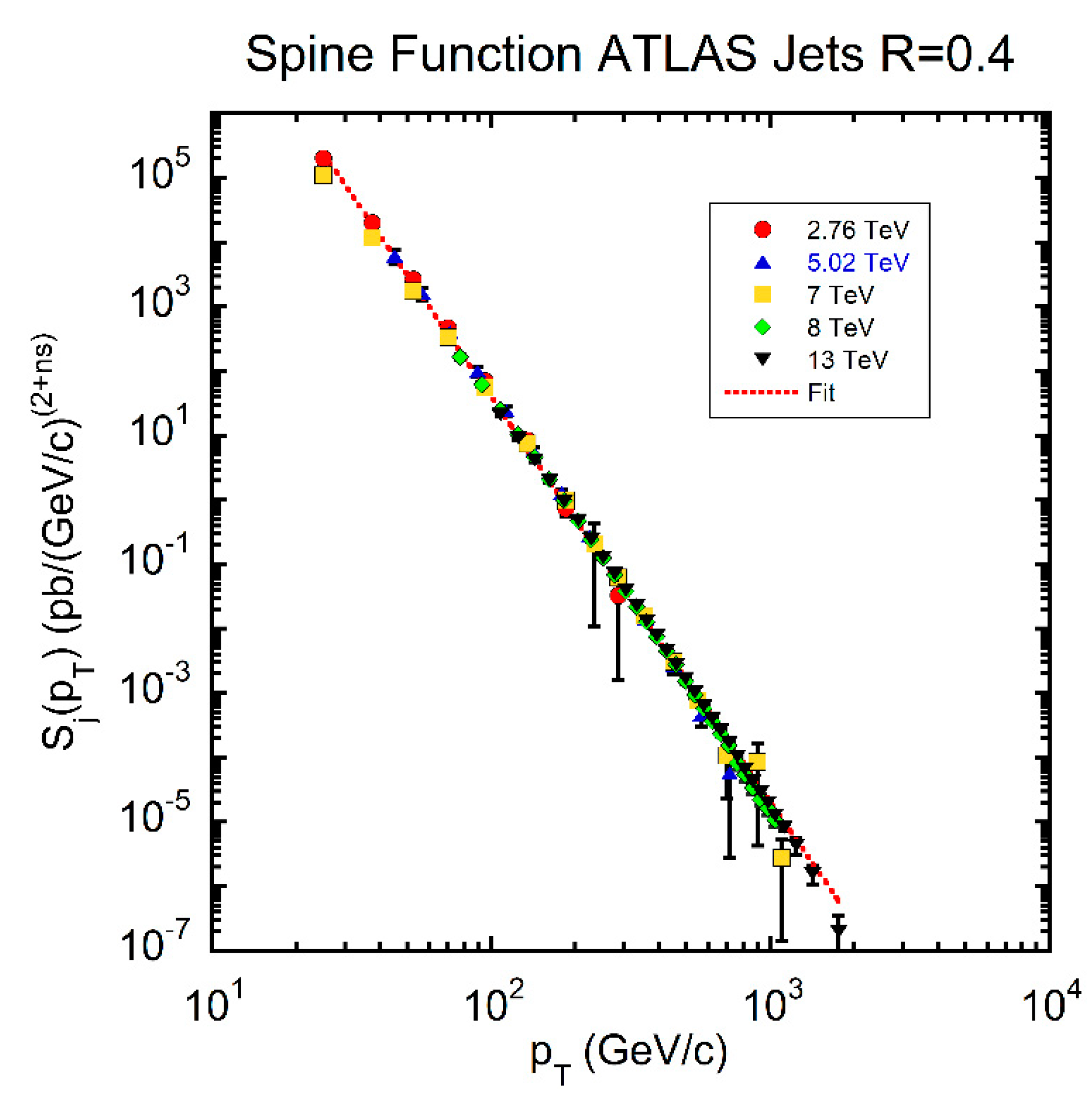
The measured dependence of inclusive jets (R = 0.4) measured at the LHC by ATLAS divided by sns/2 (called the ‘spine function’) is shown. The data are: = 2.76 TeV red circles, 5.02 TeV inverted blue triangles, 7 TeV yellow squares, 8 TeV green diamonds, 13 TeV black triangles. Note that all the data follow the same power law with = 6.29 ± 0.01. The error bars represent the statistical and systematic errors of the measurements added in quadrature. The resulting errors are mostly smaller than the plotted points. The red dotted line represents where = 2.0 ± 0.1. The data follow this power law with residuals ≤ ± 50% over 12 orders of magnitude. For plotting purposes, the error bars for 5 points were limited to no larger than 95% of the point’s value.
Figure 27.
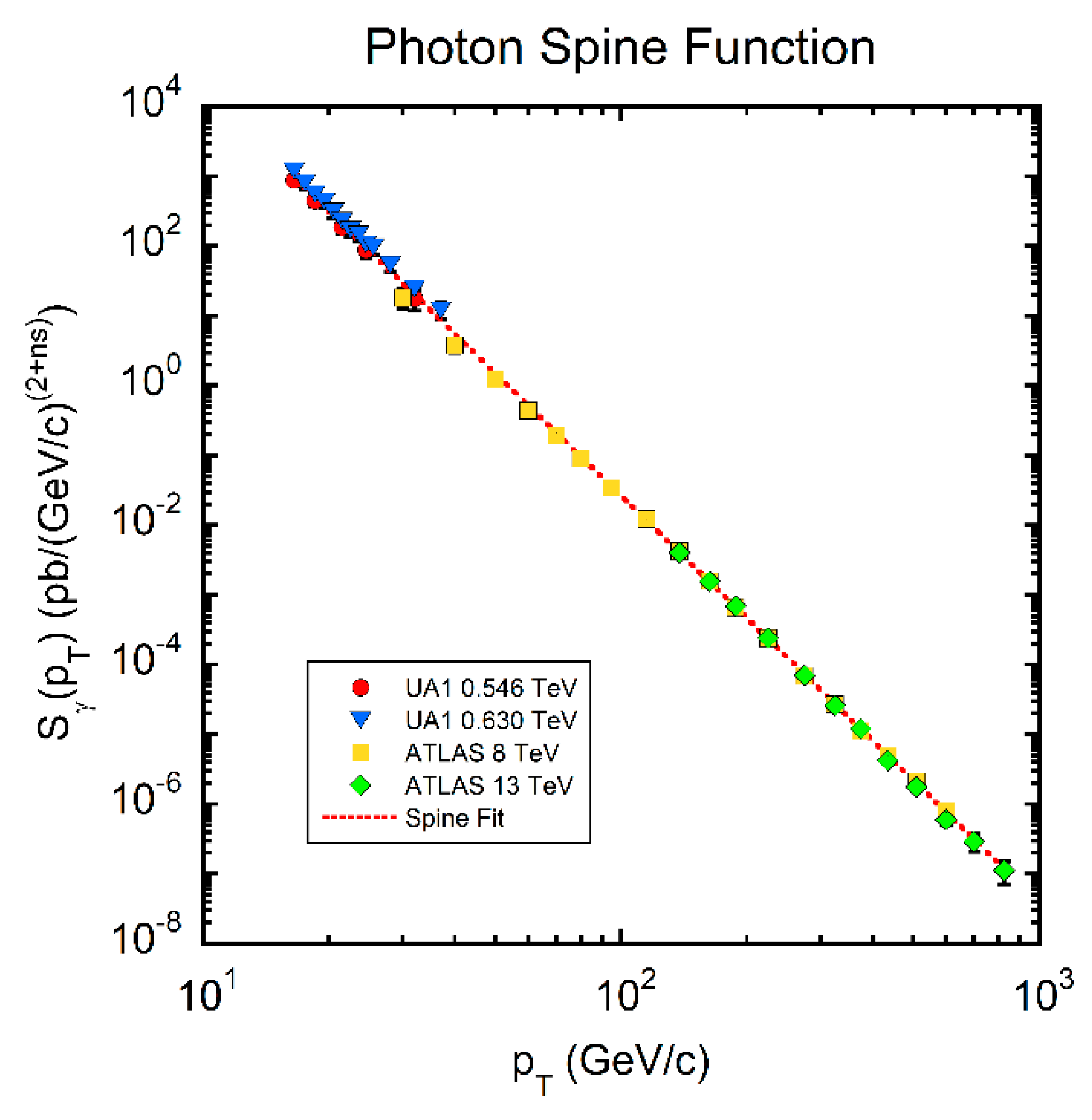
The spine function for direct photons as measured by the ATLAS and UA1 Collaboration. Data from 8 [
36] and 13 TeV [
37], yellow squares, green diamonds, respectively, are plotted. The UA1 data [
70] are represented by the red circles, blue triangles for
= 546 and 630 GeV, respectively. Error bars are plotted but are generally smaller than the symbols of the plotted points. The red dotted line represents the global fit to the ATLAS data sets. The χ
2/d.f. of the red dotted line through all the plotted points is 48/45 (
p = 0.35). Note that the UA1
= 0.546 TeV data have been normalized with respect to the ATLAS 13 TeV data by a computed factor of (13/0.546)
1.56 ~ 141.
Figure 28.
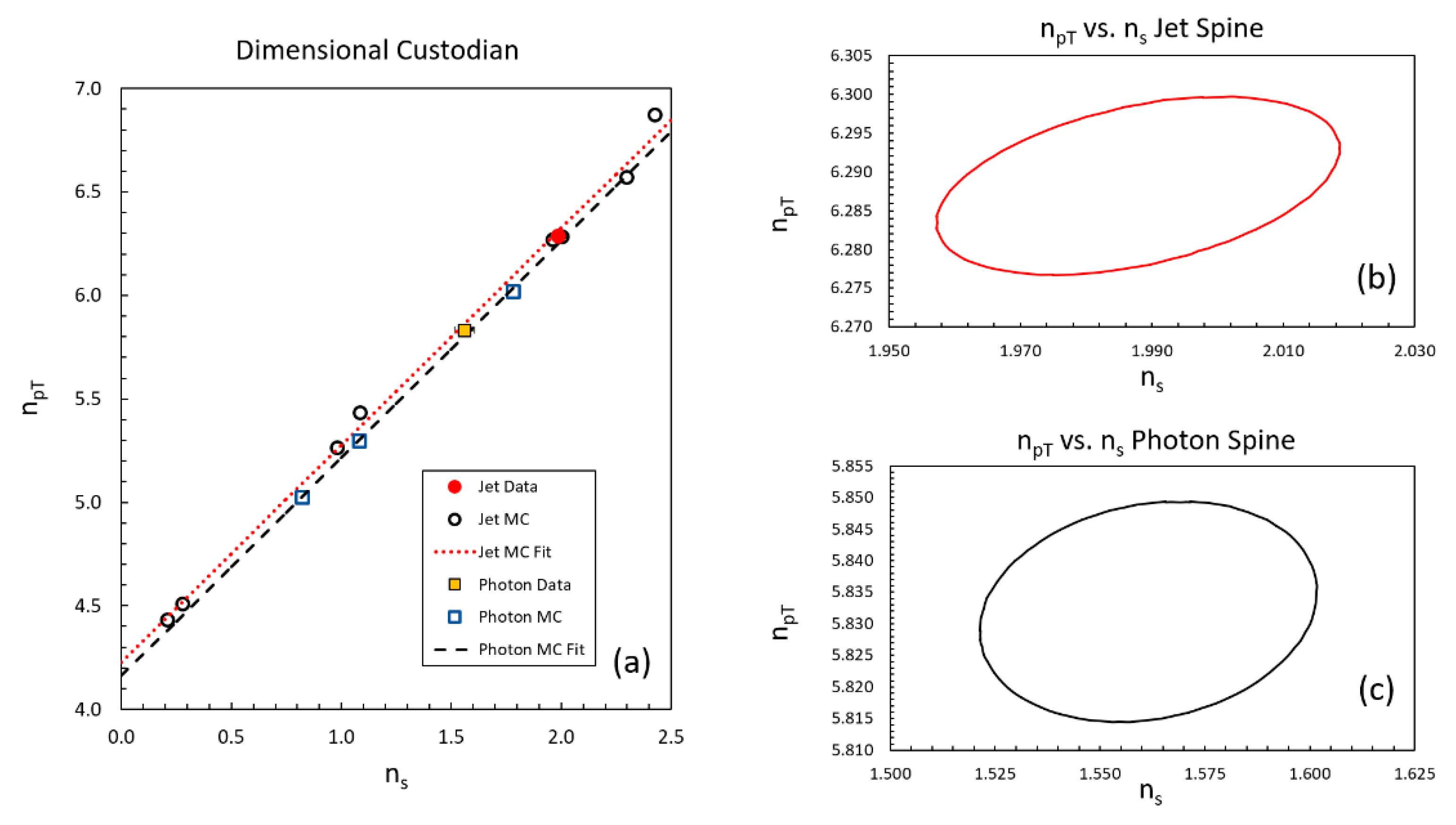
The power of
of the amplitude of the
function for inclusive cross sections is plotted against the power of the
dependence of the amplitude for data (jets red circle, photons yellow square) and simulations (jets open black circles, photons open blue squares) in (
a). Note that all values of data and MC fall on the same line indicating that the dimensions ~1/(GeV/c)
4 of the inclusive cross sections are always preserved but must include the residual
dependence from QCD evolution of the PDFs and αs(Q
2) at the
= 0 intercept for jets (red dotted line) and dashed black line for photons. The MC points include toy simulations of dijets through the
g g →
g g and
q q →
q q channels with CT10 PDF [
23] weighting as well as Pythia 8.1 inclusive jet simulations with R = 0.4 [
27]. The Toy MC considered 1.96 TeV ≤
≤ 13 TeV for the
calculation and the Pythia 8.1
value was determined from 2.76 TeV ≤
≤ 100 TeV. The photon residual power is expected to be ~½ that of jets since the QCD term is α
s(Q
2). In (
b) is plotted the 1 σ contour of the
vs.
fit for jets and in (
c) the corresponding contour for photons.
![Universe 07 00196 g028 Universe 07 00196 g028]()
Figure 29.
A comparison of
functions of jets measured by ATLAS at
= 2.76 TeV with anti-k
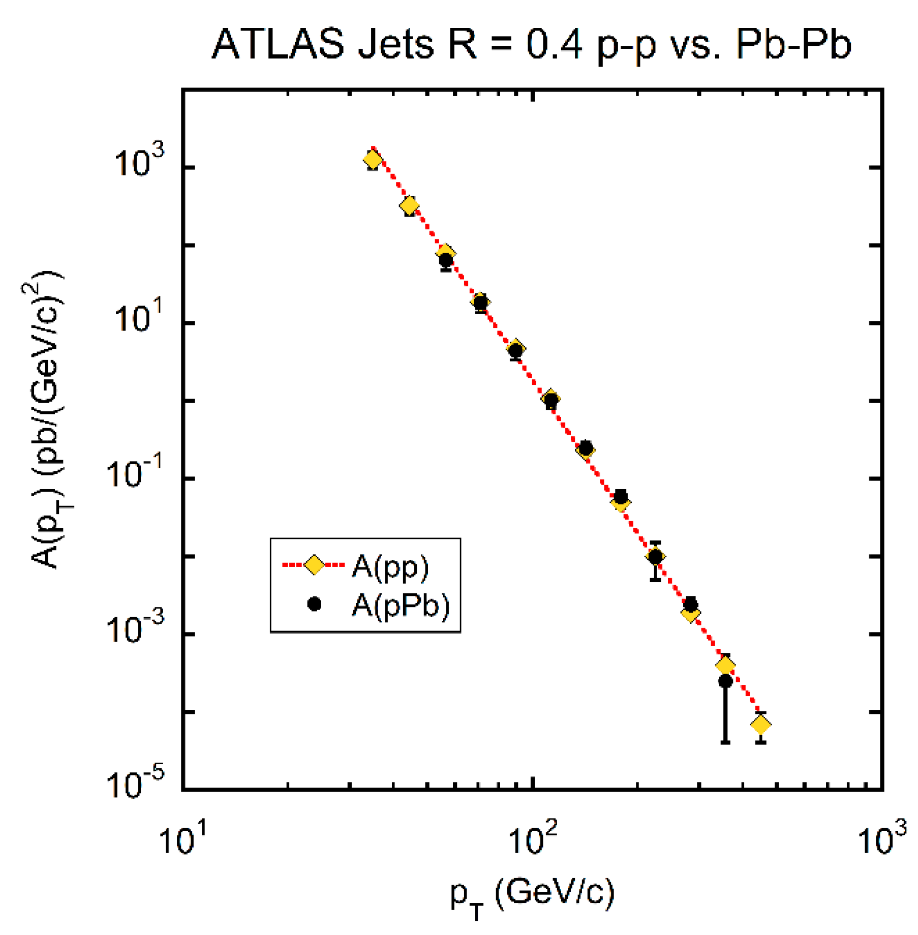
t jet definition for R = 0.4 in both p–p and Pb–Pb collisions. The p–p data are represented by yellow diamonds and the Pb–Pb data with black circles. The Pb–Pb data were normalized to the p–p data by minimizing the χ
2 of a fit to the p–p data applied to the Pb–Pb data. The red dotted line represents a power law fit to the p–p data with the average value
= 6.28 ± 0.12 (
Appendix A).
Figure 30.
Shown are the a functions plotted versus the modified transverse momentum,
, for direct J/ψ production (black points upper curve) and for decay production (red points lower curve) in p–p and p–Pb collisions measured by the LHCb collaboration. The data are consistent with pure power laws—the direct production has a larger power index than decay production. The 8 TeV p–p data have been scaled up to 8.16 TeV by adjusting κ = κ
0 (
)
ns with the computed
value computed from
by the dimensional custodial as shown in
Figure 28 and the pPb data have been divided by the nucleus A number = 208. The p–p data have a slightly smaller power index
than the corresponding pPb, Pbp data and are in good agreement with ATLAS p–p data. The error bars were computed by adding all tabulated errors in quadrature (statistical, uncorrelated systematic and correlated systematic errors).
Figure 31.
Shown is the vs. 1/ behavior of direct (a) and decay (b) production of J/ψ in p–Pb collisions compared with that of p–p collisions as measured by the LHCb collaboration. The black diamonds correspond to measurements of for p–p collisions. Shown in blue circles are the values for y* > 0 where the J/ψ is detected in the proton fragmentation hemisphere and in red triangles for y* < 0 corresponding to the Pb fragmentation region. The dotted lines indicate quadratic parameterizations that are used in the calculation of the transparency. Since each point in the figures above were computed for constant , we consider only the uncorrelated experimental errors added in quadrature.
Figure 32.
The Δ values are plotted against the modified transverse momentum for the LHCb p–p data = 8 TeV and for the p–Pb data for = 8.16 TeV for y* > 0 (a) and y* < 0 (b). The black circles are for J/ψ direct production and the red triangles are for decay production. (a) corresponds to the proton fragmentation region y* > 0, where the J/ψ has to penetrate the Pb nucleus. (b) is for the Pb fragmentation region y* < 0, where the J/ψ is co-traveling with the Pb debris. The dotted lines are quartic fits to . Since there is little difference in the two cases (direct and decay) for y* > 0 (left plot), we show a simultaneous fit to both direct and decay data sets.
Figure 33.
The transparency at = 5, 7, 9, 11 GeV/c are plotted in (a–d), respectively, as a function of rapidity y* for the LHCb heavy ion p–Pb data at = 8.16 TeV. Direct J/ψ production is represented as black circles and decay production of J/ψ by red triangles. The points below |y*| < 1.5 are extrapolation beyond the range of the LHCb data. The transparency decreases with increasing for y* > 0. The transparency becomes almost 1 for direct J/ψ production y* < 0 for > 7 GeV/c (black circles). The decay data for y* < 0, ≥ 9 GeV/c (red triangles) are consistent with a recombination process. The error bars are determined from fits to the statistical errors.
Figure 34.
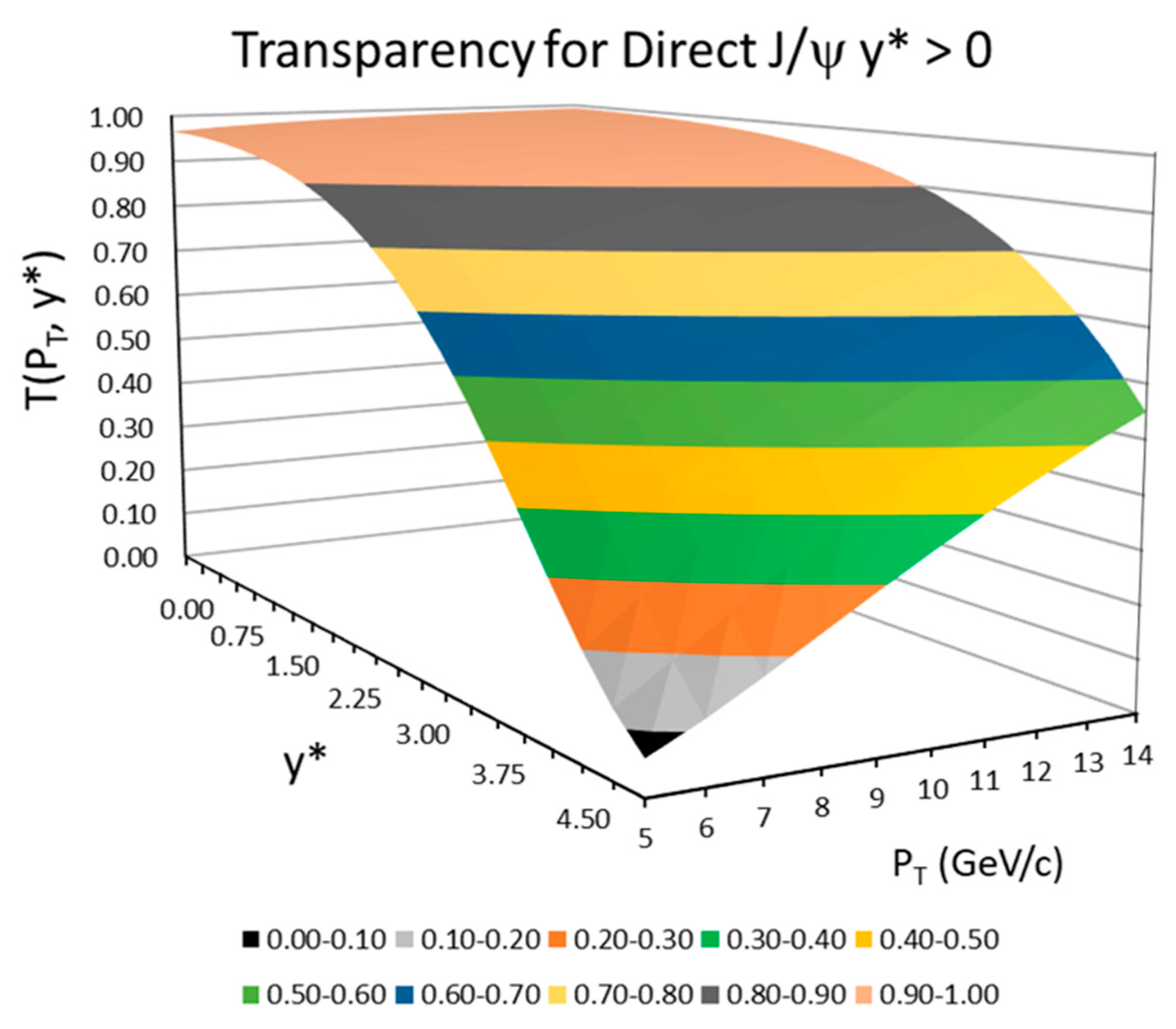
The transparency contour for direct J/ψ production as measured by the LHCb collaboration at = 8.16 TeV is shown for the y * > 0 hemisphere. The color bands correspond to contours of constant by which the transparency is calculated. The contour for y* < 1.5 is an extrapolation beyond the acceptance of the experimental data. High momentum and small y* have the largest transparency, whereas low momentum and large y* has the smallest transparency.
Figure 35.
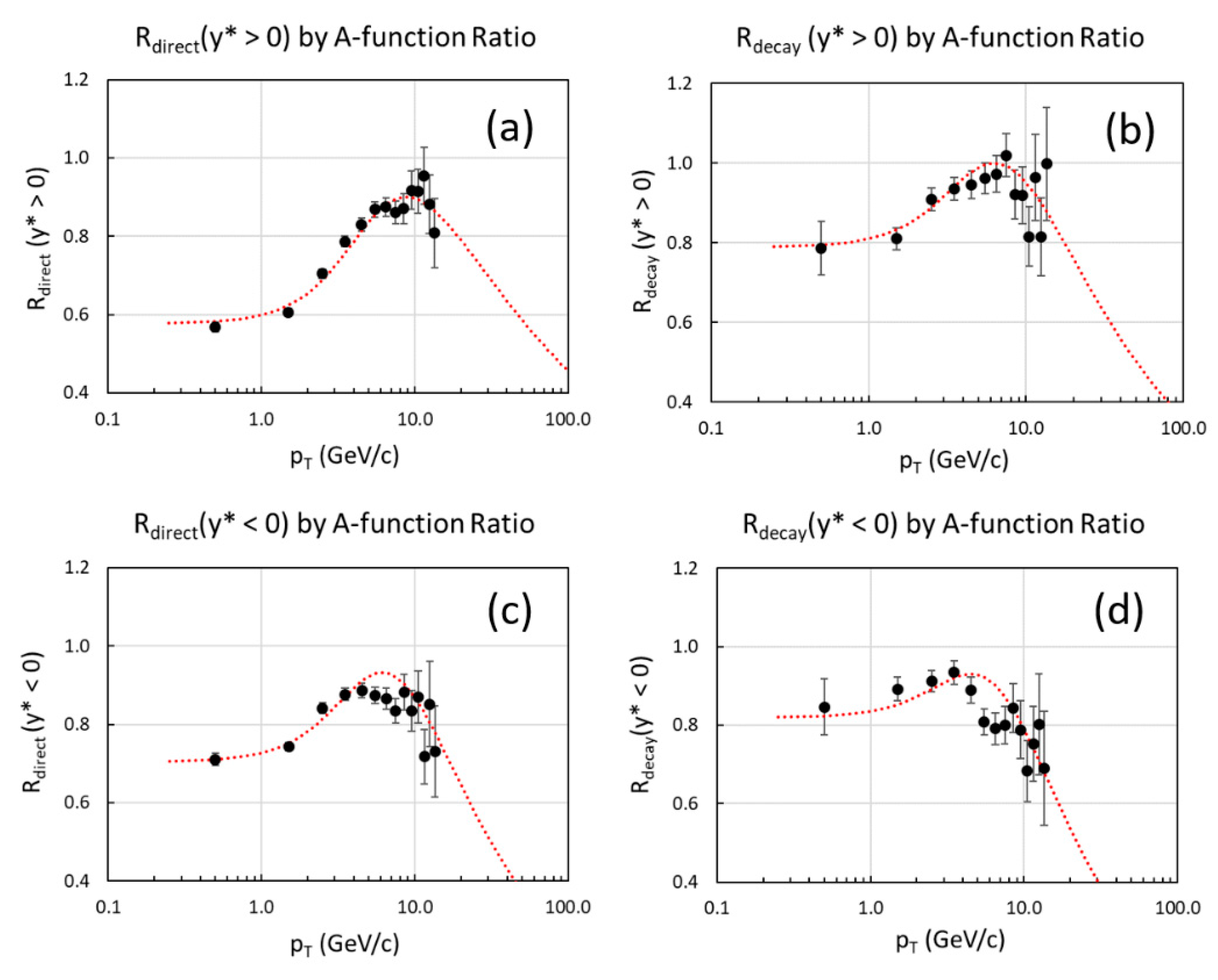
The ratio of a functions for LHCb data (back circles) as a function of vs. calculated ratio using the a function parameters (red dotted lines) given by Equation (54) extrapolated to = 100 GeV/c for each of the four combinations of direct, decay, y* > 0 (direct y* > 0 (a), decay y* > 0 (b), direct y* < 0 (c), decay y* < 0 (d)) and y* < 0 J/ψ production at = 8.16 TeV. The data in all combinations show broad peaks at ~ 6 to 9 GeV/c. Small adjustments upward in the magnitude of the red dotted curves have been made in the direct data ratios of 10% for y* > 0 and 5% for y* < 0, both well within the error caused by our using an average value for all p–Pb data and similarly for the p–p data, rather than using each value for each a function.
Table 1.
Fit parameters of 13 TeV ATLAS and CMS jets. The parameters κ and
describe the a function, and the parameters
D,
,
DQ, and
describe the
F-function. We note that the ATLAS and CMS jet parameters are consistent within errors. In the analysis of both data sets, we have required |y| ≤ 3 and have added systematic and statistical errors in quadrature. The overall normalization error in the luminosities determinations was neglected. The CERN MINUIT [
21] fitting package was used.
D and
DQ are correlated as approximately 0.5
D ~ (
DQ)
1/2.
| Experiment | Parameter | Value | χ2/d.f. | p-Value |
|---|
| ATLAS | | (2.1 ± 0.3) × 1014 pb/(GeV/c)(2-npT)
6.35 ± 0.02 | 33/29 | 0.28 |
| CMS | | (3.1 ± 1.0) × 1014 pb/(GeV/c)(2-npT)
6.41 ± 0.05 | 15/25 | 0.94 |
| ATLAS | D
| (7.0 ± 1.1) × 102 GeV/c
3.6 ± 0.2 | 14/29 | 0.99 |
| CMS | D
| (7.5 ± 3.1) × 102 GeV/c
3.3 ± 0.6 | 7/25 | 1.00 |
| ATLAS | DQ
| (1.5 ± 0.4) × 105 (GeV/c)2
0.06 ± 0.1 | 24/29 | 0.73 |
| CMS | DQ
| (2.0 ± 1.3) × 105 (GeV/c)2
0.08 ± 0.4 | 8/25 | 1.00 |
Table 2.
The cross sections for each hard-scattering process in jet production are listed showing the leading behavior at small and the values of the cross sections at the kinematic limit when . The fractional coefficients result from the various color factors of the parton–parton interactions.
Table 2.
The cross sections for each hard-scattering process in jet production are listed showing the leading behavior at small and the values of the cross sections at the kinematic limit when . The fractional coefficients result from the various color factors of the parton–parton interactions.
| Process | Leading pT Behavior | |
|---|
| | |
| | |
| | |
| | |
| | |
| | |
| | |
| | |
Table 3.
The power law indices,
of
with
≡ 0, given in Equation (3) are tabulated for the Pythia 8.1 simulation of 13 TeV jets (R = 0.4) and for our Toy MC simulation broken down for each hard-scattering process listed in
Table 2. The values of
in the Toy MC were determined from power law fits 106 GeV/c ≤
≤ 1423 GeV/c, roughly matching ATLAS data. Note that processes involving gluons and antiquarks have a larger power index than those involving quarks as would be expected from their respective PDF shapes. The power indices are constrained at 5.3 ≤
≤ 6.7. The cross section ratios for the various subprocesses to total are given in the second column. The total cross section is dominated by
and
scatterings (66% and 13% of total, respectively).
| Process | σ/σ (all) | npT |
|---|
| ATLAS | 1 | 6.35 ± 0.02 |
| CMS | 1 | 6.41 ± 0.05 |
| Pythia 8.1 | 1 | 6.31 ± 0.01 |
| All Toy | 100% | 6.35 ± 0.02 |
| 66.20% | 6.76 ± 0.03 |
| 13.09% | 6.09 ± 0.02 |
| 5.95% | 5.43 ± 0.03 |
| 3.27% | 5.33 ± 0.02 |
| 0.54% | 5.85 ± 0.03 |
| 1.98% | 6.03 ± 0.03 |
| 1.30% | 6.66 ± 0.03 |
| 0.07% | 5.54 ± 0.02 |
| 1.43% | 6.62 ± 0.04 |
| 0.81% | 6.54 ± 0.04 |
| 5.37% | 6.64 ± 0.03 |
Table 4.
The power law index of sector given in Equation (9) are tabulated for Pythia 8.1 and our Toy MC simulation for each hard-scattering process at = 13 TeV. Notice that the parameters are strongly dependent on the hard-scattering process and the underlying PDFs. Additionally, note that is strongly correlated with . The ATLAS data for D and DQ fall between the Pythia 8.1 and the Toy MC. The ATLAS, Pythia 8.1 and All Toy fits were performed by a minimum χ2 fit with MINUIT. The subprocesses were fit with linear regression (LR)—which does not minimize χ2 but does go through the points. The errors quoted for these processes are those of the LR.
| Process | D (GeV/c) | | DQ (GeV/c)2 | |
|---|
| ATLAS | 700 ± 110 | 3.6 ± 0.2 | (1.5 ± 0.4) × 105 | 0.1 ± 0.1 |
| CMS | 750 ± 307 | 3.3 ± 0.6 | (2.0 ± 1.3) × 105 | 0.1 ± 0.4 |
| Pythia 8.1 | 322 ± 30 | 4.3 ± 0.1 | (6.5 ± 1.3) × 104 | 0.4 ± 0.04 |
| All Toy | 1170 ± 92 | 3.1 ± 0.2 | (2.0 ± 0.3) × 105 | 0.4 ± 0.1 |
| 969 ± 17 | 7.1 ± 0.1 | (3.2 ± 0.03) × 105 | 1.0 ± 0.1 |
| −25 ± 46 | 4.2 ± 0.1 | (8.9 ± 0.9) × 104 | −0.2 ± 0.1 |
| −34 ± 55 | 2.7 ± 0.2 | (5.4 ± 1.1) × 104 | −1.1 ± 0.2 |
| −65 ± 52 | 3.3 ± 0.1 | (7.3 ± 1.1) × 104 | −0.8 ± 0.2 |
| 253 ± 28 | 4.7 ± 0.1 | (1.2 ± 0.1) × 105 | 0.3 ± 0.1 |
| 223 ± 40 | 4.1 ± 0.1 | (1.7 ± 0.1) × 105 | −0.2 ± 0.1 |
| 1362 ± 15 | 7.4 ± 0.1 | (4.3 ± 0.03) × 105 | 1.1 ± 0.1 |
| −169 ± 30 | 6.8 ± 0.1 | −(2.7 ± 0.7) × 104 | 0.6 ± 0.1 |
| 397 ± 34 | 8.2 ± 0.1 | (1.4 ± 0.1) × 105 | 0.6 ± 0.1 |
| 468 ± 28 | 8.7 ± 0.1 | (1.8 ± 0.1) × 105 | 0.9 ± 0.1 |
| 720 ± 18 | 8.0 ± 0.1 | (2.4 ± 0.1) × 105 | 1.2 ± 0.1 |
Table 5.
Shown are the values of the jet parameters for g g → g g scattering subprocess at = 13 TeV inclusive jet simulation by our Toy MC for two cross section definitions. The quoted errors were determined by the consistency of the fits and not by the statistics of the MC simulation. No finite bin corrections were applied. Note that η is double valued, either > 0 or < 0, whereas 0 < ≤ 1.0.
| Cross Section Definition | | |
|---|
| 6.76 ± 0.03 | 6.59 ± 0.02 |
| 6.83 ± 0.04 | 7.3 ± 0.1 |
| 1.04 ± 0.04 | 0.1 ± 0.1 |
| D (GeV/c) | 948 ± 17 | 950 ± 37 |
| DQ (GeV/c)2 | (3.01 ± 0.03) × 105 | (2.98 ± 0.08) × 105 |
Table 6.
The
, expressed in GeV, dependence of the parameters
κ(
),
D(
s) and
DQ(
s) are tabulated. The data were fit assuming all five
points are of equal statistical weight. For the
κ(
s) parameter, the Monte Carlo simulations (Pythia 8.1, Toy) were normalized to the
= 13 TeV data point. In summary, it appears that
κ(
s) and
DQ(
s) increase with a power ~2, whereas
D(s) increases with a power ~1, that is linearly in
. It is apparent from
Figure 10 that there is considerable scatter in the parameter values of the jet fits so for the logarithmic behavior of the parameters with respect to ln(
) we quote the regression value, R
2, instead of the χ
2/d.f.
| Parameter | Power Index | Constant Term | R2 |
|---|
| κ(s) | ns | ln(κ0) | |
| Data | 2.3 ± 0.7 | 11 ± 6 | 0.79 |
| Pythia 8.1 | 2.4 ± 0.2 | 10.2 ± 1.7 | 0.98 |
| Toy | 2.5 ± 0.3 | 9 ± 3 | 0.96 |
| D(s) | nD | ln(D0) | |
| Data | 0.9 ± 0.5 | −2 ± 5 | 0.51 |
Pythia 8.1
≥ 7 TeV | 1.1 ± 0.1 | −5.1 ± 0.8 | 0.99 |
| Toy | 1.0 ± 0.1 | −3.0 ± 0.1 | 0.96 |
| DQ(s) | nDQ | ln(DQ0) | |
| Data | 2.3 ± 1.0 | −10 ± 9 | 0.63 |
Pythia 8.1
≥ 7 TeV | 2.2 ± 0.1 | −9.6 ± 0.9 | 0.99 |
| Toy | 2.0 ± 0.5 | −8 ± 5 | 0.84 |
Table 7.
The power indices , and of data averaged over 2.76 ≤ ≤ 13 TeV of inclusive jets (R = 0.4) measured by ATLAS are compared with two MC simulations and are tabulated. The quoted errors are the standard deviation about the average. The Monte Carlo simulations, Pythia 8.1 and Toy MC are in good agreement with data and are consistent with the and data values, for the later within 50% errors.
| Parameter | Average Value | Data/MC |
|---|
| | | |
| Data | 6.3 ± 0.1 | |
| Pythia 8.1 | 6.28 ± 0.04 | 1.00 ± 0.02 |
| Toy MC | 6.27 ± 0.06 | 1.00 ± 0.02 |
| | | |
| Data | 3.7 ± 0.4 | |
| Pythia 8.1 | 4.4 ± 0.2 | 0.8 ± 0.1 |
| Toy MC | 3.92 ± 0.04 | 0.9 ± 0.1 |
| | | |
| Data | 0.4 ± 0.2 | |
| Pythia 8.1 | 0.4 ± 0.1 | 0.8 ± 0.6 |
| Toy MC | 0.62 ± 0.01 | 0.6 ± 0.4 |
Table 8.
The χ
2 values of comparison of data with themselves vs. data with the Toy MC and Pythia 8.1 simulations of data shown in
Figure 13. In all comparisons, the
and
values were used for the model. The column “Data” is the comparison of actual data points with the model determined by Equation (13). The χ
2 values and the numbers of degrees of freedom are shown as ratio and value for each comparison: data vs. data, data vs. Toy MC and data vs. Pythia 8.1. The errors used in the χ
2 computation include the errors of the fit as well as data systematic and systematic errors added in quadrature.
p-Values less than 10
−8 were set to 0.
| Data | | Toy MC | | Pythia 8.1 MC | |
|---|
| | χ2/d.f. | p-Value | χ2/d.f. | p-Value | χ2/d.f. | p-Value |
|---|
| 2.76 TeV ATLAS | 21.2/52 | 1.00 | 71/52 | 0.04 | 130/52 | 1.3 × 10⁻⁸ |
| 5.02 TeV ATLAS | 14.1/72 | 1.00 | 149/72 | 2.7 × 10⁻⁷ | - | - |
| 7 TeV* ATLAS | 15.0/83 | 1.00 | 51.3/83 | 0.99 | 50.3/83 | 0.99 |
| 8 TeV ATLAS | 161/155 | 0.35 | 3464/155 | 0 | - | - |
| 13 TeV ATLAS | 137/171 | 0.97 | 1161/171 | 0 | 771/171 | 0 |
| 13 TeV CMS | 143/154 | 0.73 | 248/154 | 2.4 × 10⁻⁶ | 494/154 | 0 |
Table 9.
The various parton–parton scattering processes (carets not shown) that contribute to direct photon production in p–p scattering are listed. The leading
dependences at small
and the values of the cross sections at the kinematic limit where
are shown. The
cross section depends on both
αe and
αs and on s, t, and u through the terms T
i. This channel was neglected since it contributes ≤ 0.1% of the overall production cross section. In all cases, the exact expressions for the scattering cross sections were used in the Toy MC simulations. The expressions shown here are only to give a rough idea of the
and
dependences. Notice that, unlike the cross sections of
Table 2, the photon-producing cross sections are
dependent and at low
and fall with increasing
as
.
| Process | Leading pT | |
|---|
| | |
| | |
| | |
| | See Owens [25] (neglected) |
Table 10.
The contributions of each process, σ(i), operative in the production of direct photons at = 8 and 13 TeV integrated over 34.8 ≤ ≤ 990 GeV/c and 138.3 ≤ ≤ 1932 GeV/c for our Toy MC 8 and 13 TeV simulations, respectively, and over 0 ≤ |y| ≤ 2.5 for both energies are shown along with their corresponding power law indices. The power law indices were calculated for MC data in the range 34.8 ≤ ≤ 600 GeV/c and 138.3 ≤ ≤ 1310 GeV/c for 8 and 13 TeV data, respectively, which roughly corresponds to the ATLAS data ranges. The g g → γγ process is neglected. The Toy MC is only useful as a rough guide—it underestimates the value of by approximately 11%. There is a small dependence in the fractional contributions to the total cross section but the values of for all processes change by only 0.56%.
| | 8 TeV | | 13 TeV | |
|---|
| Process | σ (i)/σ (All) | npT | σ (i)/σ (All) | npT |
|---|
| All | 100% | 5.35 ± 0.01 | 100% | 5.32 ± 0.01 |
| 89.01% | 5.40 ± 0.01 | 85.52% | 5.35 ± 0.01 |
| 10.80% | 5.11 ± 0.01 | 14.19% | 5.19 ± 0.01 |
| 0.19% | 4.95 ± 0.01 | 0.29% | 5.01 ± 0.01 |
Table 11.
The leading order cross sections and their behavior at low
and at the kinematic boundary are tabulated. Again, the carets denoting variables of parton–parton scattering have been omitted. The equations were derived from [
43] and checked with those in the PDG [
26]. The modified transverse momentum
.
| Process | Leading pT | |
|---|
| | |
| | |
Table 12.
Spine function parameters for inclusive jets. Data are compared with Toy MC and Pythia 8.1 simulations. The Toy simulation had the relative errors of simulated invariant cross section ‘data’ points fixed to 2%, whereas the errors of the Pythia 8.1 simulation itself were used. Since the MCs have no absolute normalizations, the values of κ0 for them are arbitrary and therefore not tabulated. The MC fits ranged from 2.76 ≤ ≤ 13 TeV matching the range of data. The and |y| binning of the MC simulations were forced to be the same as data.
| Inclusive Jets | Parameter | Value |
|---|
| Data | κ0 | (10 ± 3) × 105 (pb GeV(npT-ns−2)) |
| Data | | 1.99 ± 0.04 |
| Toy MC | | 2.084 ± 0.004 |
| Pythia 8.1 MC | | 2.028 ± 0.005 |
| Data | | 6.29 ± 0.01 |
| Toy MC | | 6.286 ± 0.002 |
| Pythia 8.1 MC | | 6.243 ± 0.003 |
| Data | | 0.30 ± 0.04 |
| Toy MC | | 0.203 ± 0.004 |
| Pythia 8.1 MC | | 0.216 ± 0.005 |
| Data | χ2/d.f. | 221/94 (p = 3 × 10⁻¹²) |
Table 13.
Spine function parameters for inclusive photons. Data are compared with Toy MC simulation through the parameters , and . The MC simulation has the relative errors of invariant differential cross section fixed to 2%. The simulation was from 2.76 ≤ ≤ 13 TeV, whereas the data were 8 ≤ ≤ 13 TeV. Since the MC had no absolute normalization, the values of κ0 for them are arbitrary and therefore not tabulated. The and y binning of the MC simulation were forced to be the same as data.
| Inclusive Photons | Parameter | Value |
|---|
| Data | κ0 | (5 ± 2) × 103 (pb (GeV/c)(npT-ns−2)) |
| Data | | 1.56 ± 0.04 |
| Toy MC | | 1.08 ± 0.01 |
| Data | | 5.83 ± 0.02 |
| Toy MC | | 5.30 ± 0.01 |
| Data | | 0.27 ± 0.05 |
| Toy MC | | 0.22 ± 0.01 |
| Data | χ2/d.f. | 44/27 (p = 0.02) |
| Toy MC | χ2/d.f. | 277/95 (p = 1 × 10⁻¹⁹) |
Table 14.
The parameters of the dependence of J/ψ production in p–p and p–Pb collisions. The p–p data were taken at = 8.0 TeV and the p–Pb and Pb–p data were taken at a nucleon–nucleon COM energy = 8.16 TeV. The values of κ for p–Pb collisions have been normalized to per nucleon by dividing by A = 208. The numbers tabulated were computed with uncorrelated systematic errors added in quadrature with statistical errors. The correlated systematic errors were not included. The values of κ were computed with the weighted averages of = (4.1 ± 0.1) GeV/c for p–p data and = (4.7 ± 0.1) GeV/c for p–Pb data. The p–p values tend to be smaller than those of p–Pb and Pb–p collisions by 1.7σ for direct production and 1.3σ for decay production.
| Process | y Range | Λm (GeV/c) | npT | κ (nb/(GeV/c)2) |
|---|
| Direct p–p | 2.0 < y* < 4.5 | 4.1 ± 0.2 | 6.9 ± 0.3 | (4.7 ± 0.2) ×106 |
| Direct p–Pb | 1.5 < y* < 4.0 | 4.8 ± 0.2 | 7.5 ± 0.2 | (1.2 ± 0.1) × 107 |
| Direct Pb–p | −5.0 < y* < −2.5 | 4.6 ± 0.1 | 7.5 ± 0.2 | (2.3 ± 0.2) × 107 |
| Decay p–p | 2.0 < y* < 4.5 | 4.1 ± 0.1 | 5.6 ± 0.1 | (8.0 ± 0.3) × 104 |
| Decay p–Pb | 1.5 < y* < 4.0 | 4.6 ± 0.3 | 6.0 ± 0.3 | (2.7 ± 0.2) × 105 |
| Decay Pb–p | −5.0 < y* < −2.5 | 4.3 ± 0.3 | 5.9 ± 0.3 | (4.2 ± 0.6) × 105 |


