Shaping Dynamical Casimir Photons

Abstract

Temporal modulation of the quantum vacuum through fast motion of a neutral body or fast changes of its optical properties is known to promote virtual into real photons, the so-called dynamical Casimir effect. Empowering modulation protocols with spatial control could enable the shaping of spectral, spatial, spin, and entanglement properties of the emitted photon pairs. Space–time quantum metasurfaces have been proposed as a platform to realize this physics via modulation of their optical properties. Here, we report the mechanical analog of this phenomenon by considering systems in which the lattice structure undergoes modulation in space and in time. We develop a microscopic theory that applies both to moving mirrors with a modulated surface profile and atomic array meta-mirrors with perturbed lattice configuration. Spatiotemporal modulation enables motion-induced generation of co- and cross-polarized photon pairs that feature frequency-linear momentum entanglement as well as vortex photon pairs featuring frequency-angular momentum entanglement. The proposed space–time dynamical Casimir effect can be interpreted as induced dynamical asymmetry in the quantum vacuum.

1. Introduction

The generation of photon pairs out of the quantum vacuum, the so-called dynamical Casimir effect (DCE), was originally described as a motion-induced phenomenon [1], but it can occur when any kind of temporal modulation is exerted on the vacuum to promote virtual photons as real photons [2,3,4,5]. Motion-induced photon generation has not been observed to date because it requires unfeasibly large modulation frequencies of a mechanical boundary, and several analog DCE systems have been demonstrated involving temporal modulation of material properties [6,7,8,9]. Still, the physics of motional dynamical Casimir effects offers interesting insights into the interplay between matter and field fluctuations in non-equilibrium systems. Motional DCE (also known as motion-induced or mechanical DCE) is typically described in a “field-centric” approach based on quantum fluctuations of the electromagnetic field supplemented with time-dependent boundary conditions. A “matter-centric” approach has been recently pursued based on microscopic models that emulate a moving dielectric mirror as a collection of accelerated dipoles that emit quantum radiation [10]. Interestingly, the two descriptions result in identical predictions for the angular emission profile of DCE photons. This duality between field-centric and matter-centric approaches also occurs in equilibrium fluctuation-induced interactions [11]. Microscopic models can be used to study the dissipative counterpart of DCE emission, namely the drag force on the moving mirror as well as the related problem of quantum friction and associated near-field DCE emission of surface polaritons [12,13].

Modulation protocols with both temporal and spatial control can enable novel functionalities such as the generation of complex structured Casimir light. We recently proposed an analog dynamical Casimir effect based on the concept of space–time quantum metasurfaces [14], in which the optical properties of a quantum metasurface are modulated in space and time and generate DCE photon pairs with tailored spatial profiles at giant production rates. Here, we develop the motion-induced version of this effect based on a microscopic model of a spatiotemporally modulated mirror. We describe the mirror as a collection of dipoles in which the center-of-mass coordinates are modulated in space and in time and find that photon pairs are generated out of vacuum with tailored spatial modes determined by the spatial modulation protocol. The collection of dipoles behaves as a quantum phase array antenna that emits structured Casimir light. The same microscopic theory applies to a quantum meta-mirror comprising an atomic array with modulated lattice structure [15]. We call the proposed effect space–time DCE to distinguish it from the standard DCE process that involves temporal modulation only.

2. Materials and Methods

2.1. Microscopic Model for Space–Time Motional DCE

A microscopic model for a spatiotemporally modulated dielectric mirror consists of an array of N multi-level atoms, each of which undergoes its own accelerated trajectory ${\mathbf{R}}_j\left(t\right)$ and couples to the electromagnetic field via the dipolar interaction. The trajectories are driven by some external agent, and in this work, we consider oscillatory trajectories typically employed in studies of the dynamical Casimir effect. We note, however, that our theory can be extended to arbitrary trajectories. The spatial modulation is incorporated via a synthetic phase $\mathsf{\Phi }\left({\mathbf{R}}_j\right)$ that is imprinted by a temporal delay of the oscillation of each atom. We thus consider

$${\mathbf{R}}_j\left(t\right)={\mathbf{R}}_j+\widehat{\mathbf{z}}\Delta cos(\mathsf{\Omega }t-\mathsf{\Phi }\left({\mathbf{R}}_j\right)),$$

(1)

where ${\mathbf{R}}_j$ is the static position of the jth atom ($j=1,\dots ,N)$, $\Delta$ is the oscillation amplitude, and $\mathsf{\Omega }$ is the oscillation frequency. A conceptual representation of the spatiotemporally modulated atoms is shown in Figure 1. For example, a traveling-wave modulation on the $x-y$ plane corresponds to $\mathsf{\Phi }\left({\mathbf{R}}_j\right)=\mathit{\beta }·{\mathbf{r}}_j$ with ${\mathbf{r}}_j=(x_j,y_j)$ and $\mathit{\beta }=({\beta }_x,{\beta }_y)$ being momentum “kicks” on the same plane. A spinning-wave modulation around an axis orthogonal to the mirror’s plane corresponds to $\mathsf{\Phi }\left({\mathbf{R}}_j\right)=\ell {\phi }_j$, where ℓ is an integer denoting an imprinted angular momentum and ${\phi }_j$ is the azimuthal coordinate of each atom. Note that, under this modulation, the atoms are not rotating but the temporal dephasing of their oscillatory motion along the z direction is spinning around the $z-$ axis. The traveling-wave modulation could be implemented by an acoustic perturbation that launches a plane-wave on the surface of the mirror. In the case of a meta-mirror formed by an atomic array monolayer trapped in a three-dimensional deep optical lattice, the modulation could be accomplished by shaking the vertical lattice and by using spatial light modulators to set a phase shift among the vertical trapping fields on different atoms to imprint the linear synthetic phase.

The dipole array interacts with the electromagnetic field via the Hamiltonian (SI units used throughout):

$$H\left(t\right)=-\sum _j{\mathbf{d}}_j\left(t\right)·\left[\mathbf{E}({\mathbf{R}}_j\left(t\right),t)+{\mathbf{v}}_j\left(t\right)\times \mathbf{B}({\mathbf{R}}_j\left(t\right),t)\right],$$

(2)

where ${\mathbf{d}}_j\left(t\right)$ is the electric dipole operator of atom j, $\mathbf{E}(\mathbf{R},t)$ and $\mathbf{B}(\mathbf{R},t)$ are the electric and magnetic fields both evaluated at the atomic positions, and ${\mathbf{v}}_j\left(t\right)=-\widehat{\mathbf{z}}\mathsf{\Omega }\Delta sin(\mathsf{\Omega }t-\mathsf{\Phi }\left({\mathbf{R}}_j\right))$ is the (non-relativistic) velocity of each atom. In this paper, the atomic internal degrees of freedom and the electromagnetic field are treated as quantum dynamical variables while the atomic center-of-mass is a classical prescribed motion. The first term in the Hamiltonian is the usual electric dipole interaction, and the second is the so-called Röntgen interaction. We note that the Röntgen term must be taken into account in the DCE far-field emission of photons, as we study here. For the DCE problem of emission in the near-field, e.g., pairs of surface polaritons induced on a surface by a close-by moving atom, it can be neglected [12,13]. The non-zero matrix elements of the electric dipole operator ${\mathbf{d}}_j\left(t\right)$ in the interaction picture are

$$\langle g_j|{\mathbf{d}}_j\left(t\right)|e_j\rangle ={\widehat{\eta }}_j{d}_{eg}{e}^{-i{\omega }_{eg}t},$$

(3)

where $|g_j\rangle$ is the ground state of atom j, $|e_j\rangle$ is an excited state, $\widehat{\eta }$ is a real unit vector denoting the orientation of the jth dipole, and $d_{eg}$ is the matrix element. Note that all atoms have the same $d_{eg}$ as we assume identical atoms and that we are not restricted to two-level atoms.When the atoms are isotropic, the sum over orientations of any given atom gives ${\sum }_{{\widehat{\eta }}_j}{\left({\eta }_j\right)}_a{\left({\eta }_j\right)}_b={\delta }_{ab}$. We consider that the atoms are sufficiently spaced within the array to neglect multiple scattering of photons among different atoms, rendering the evolution of different atoms identical irrespective of their location within the array. The electromagnetic field in the interaction picture is then simply given by the free field that we expand in a set of modes in the usual way:

$$\begin{array}{ccc}\hfill \mathbf{E}(\mathbf{R},t)& =& i\sum _{\gamma }{\left(\frac{\hslash {\omega }_{\gamma }}{2{ϵ}_{0}V}\right)}^{1/2}[{\mathbf{E}}_{\gamma }\left(\mathbf{R}\right)a_{\gamma }{e}^{-i{\omega }_{\gamma }t}-{\mathbf{E}}_{\gamma }^{*}\left(\mathbf{R}\right)a_{\gamma }^{†}{e}^{i{\omega }_{\gamma }t}],\hfill \end{array}$$

$$\begin{array}{ccc}\hfill \mathbf{B}(\mathbf{R},t)& =& \sum _{\gamma }{\left(\frac{\hslash }{2{ϵ}_{0}V{\omega }_{\gamma }}\right)}^{1/2}[\nabla \times {\mathbf{E}}_{\gamma }\left(\mathbf{R}\right)a_{\gamma }{e}^{-i{\omega }_{\gamma }t}+\nabla \times {\mathbf{E}}_{\gamma }^{*}\left(\mathbf{R}\right)a_{\gamma }^{†}{e}^{i{\omega }_{\gamma }t}].\hfill \end{array}$$

(4)

Here, V is a quantization volume, ${\mathbf{E}}_{\gamma }\left(\mathbf{R}\right)$ is the spatial mode, ${\omega }_{\gamma }>0$ is the mode frequency, and $a_{\gamma }^{†}$ and $a_{\gamma }$ are creation and annihilation operators of photons in mode $\gamma$. The specific choice of modes is determined by the symmetries of the synthetic phase, as we discuss later in the paper.

2.2. Two-Photon Emission Rate

We assume that the initial state of the N-atom system plus electromagnetic field is all of the identical atoms in their ground state and the field in vacuum, i.e., $\left|\psi \right(0)\rangle =|\left\{g\right\};vac\rangle$, where we denote $|\left\{g\right\}\rangle =|g_1,g_2,\dots ,g_N\rangle$ as the multi-atom ground state. The time-evolved state in the interaction picture to second order in the dipolar couplings $d_{eg}$ is

$$\begin{array}{ccc}& & |\psi \left(t\right)\rangle \approx c_0\left(t\right)|\left\{g\right\};vac\rangle +\sum _j\sum _{e_j,{\widehat{\eta }}_j}\sum _{\gamma }{c}_{\gamma }^{\left(e_j\right)}\left(t\right)|e_j,{\left\{g\right\}}_j;\gamma \rangle \hfill \\ & & +\sum _{j\ne j^{\prime }}\sum _{e_j,{\widehat{\eta }}_j}\sum _{e_{j^{\prime }},{\widehat{\eta }}_{j^{\prime }}}\sum _{{\gamma }_1,{\gamma }_2}{c}_{{\gamma }_1,{\gamma }_2}^{(e_j,e_{j^{\prime }})}\left(t\right)|e_j,e_{j^{\prime }},{\left\{g\right\}}_{j,j^{\prime }};{\gamma }_1,{\gamma }_2\rangle \hfill \\ & & +\sum _{j\ne j^{\prime }}\sum _{e_j,{\widehat{\eta }}_j}\sum _{e_{j^{\prime }},{\widehat{\eta }}_{j^{\prime }}}{c}_0^{(e_j,e_{j^{\prime }})}\left(t\right)|e_j,e_{j^{\prime }},{\left\{g\right\}}_{j,j^{\prime }};vac\rangle +\frac{1}{2}\sum _{{\gamma }_1,{\gamma }_2}{c}_{{\gamma }_1,{\gamma }_2}\left(t\right)|\left\{g\right\};{\gamma }_1,{\gamma }_2\rangle .\hfill \end{array}$$

(5)

We denote $|e_j,{\left\{g\right\}}_j\rangle =|g_1,\dots ,g_{j-1},e_j,g_{j+1},\dots ,g_N\rangle$ as the state in which one atom is excited and $|e_j,e_{j^{\prime }},{\left\{g\right\}}_{j,j^{\prime }}\rangle =|g_1,\dots ,g_{j-1},e_j,g_{j+1},\dots ,g_{j^{\prime }-1},e_{j^{\prime }},g_{j^{\prime }+1},\dots ,g_N\rangle$ as the state in which two atoms are excited. We make the crucial assumption that the modulation frequency is much smaller than any atomic transition frequency from the ground state, $\mathsf{\Omega }\ll {\omega }_{eg}$. In this approximation, the second, third, and fourth terms give transition amplitudes that are non-resonant and their contributions to the process of one- and two-photon generation are negligible and discarded in the following. In this regime, the DCE process is solely given by the fifth term, for which photon pairs are generated, and all atoms remain in their ground state.

One can compute the transition amplitude $c_{{\gamma }_1,{\gamma }_2}\left(t\right)$ in two ways: (a) use second-order time-dependent perturbation theory based on the bilinear Hamiltonian $H\left(t\right)$ that depends on field and atomic degrees of freedom or (b) use first-order time-dependent perturbation theory based on an effective Hamiltonian $H_{eff}\left(t\right)$ that depends quadratically on field degrees of freedom and contains information about the atoms through their ground-state polarizability. Approach (b) was used in [10] for the case of a single atom and no synthetic phase: the atom-field interaction was written in the atom’s co-moving frame as the standard static dipolar interaction; it was then re-written as an effective Hamiltonian that traces over the atom’s internal degrees of freedom rendering the interaction quadratic in the field and depending on the atomic ground-state dynamic polarizability; and finally, the Hamiltonian was Lorentz boosted to the lab frame to get $H_{eff}\left(t\right)$. Although approach (b) is technically simple, it has the drawback that it obscures the joint atom-field dynamics. Furthermore, for multiple atoms and non-zero synthetic phases, it requires the introduction of multiple co-moving frames because atoms in the array have different instantaneous velocities. For these reasons, in this work, we prefer to follow the physically more transparent albeit more cumbersome approach (a).

The transition amplitude is given by the usual expression in second-order time-dependent perturbation theory:

$$c_{{\gamma }_1,{\gamma }_2}\left(t\right)=-\frac{1}{{\hslash }^2}{\int }_0^{t}d{t}^{\prime }{\int }_0^{t^{\prime }}d{t}^{″}\sum _j\sum _{e_j,{\widehat{\eta }}_j\gamma }\langle \left\{g\right\};{\gamma }_1,{\gamma }_2|H\left(t^{\prime }\right)|e_j,{\left\{g\right\}}_j;\gamma \rangle \langle e_j,{\left\{g\right\}}_j;\gamma |H\left(t^{″}\right)|\left\{g\right\};vac\rangle$$

(6)

which sums over intermediate virtual states $|e_j,{\left\{g\right\}}_j;\gamma \rangle$. In the limit, when the relevant field wavelengths are much larger than the atomic displacements, $\omega \Delta /c\ll 1$, we can approximate the Röntgen term of the Hamiltonian by evaluating the fields at the static atomic positions, so that it has a time-dependency $\sim sin(\mathsf{\Omega }t-\mathsf{\Phi }\left({\mathbf{R}}_j\right))$ arising from the velocity. Additionally, the dipolar term in the Hamiltonian can be expanded around the equilibrium positions, giving a time-dependency $\sim cos(\mathsf{\Omega }t-\mathsf{\Phi }\left({\mathbf{R}}_j\right))$ from the spatial gradient of the field. After these approximations, the concatenated time integrals in Equation (6) can be readily evaluated as they are reduced to integrals of products of simple harmonic functions. The final result is a sum of various terms that oscillate in time. We drop the co-rotating term $e^{i({\omega }_1+{\omega }_2+\mathsf{\Omega })t}$ because it averages out to zero, and we focus on frequencies ${\omega }_{1,2}\le \mathsf{\Omega }\ll {\omega }_{eg}$ for which the only counter-rotating term that gives a resonant contribution is ${({\omega }_1+{\omega }_2-\mathsf{\Omega })}^{-1}\times e^{i({\omega }_1+{\omega }_2-\mathsf{\Omega })t}$. Upon using all of these considerations, the transition amplitude results

$$\begin{array}{ccc}\hfill c_{{\gamma }_1,{\gamma }_2}^{\left(\mathsf{\Phi }\right)}\left(t\right)& \approx & e^{i({\omega }_1+{\omega }_2-\mathsf{\Omega })t/2}\frac{\mathsf{\Omega }\Delta \sqrt{{\omega }_1{\omega }_2}}{2cV}\left(\sum _e\frac{2d_{eg}^2}{3{ϵ}_0\hslash {\omega }_{eg}}\right)\frac{sin[({\omega }_1+{\omega }_2-\mathsf{\Omega })t/2]}{{\omega }_1+{\omega }_2-\mathsf{\Omega }}\hfill \\ & & \times \sum _j{e}^{i\mathsf{\Phi }\left({\mathbf{R}}_j\right)}{W}_{{\gamma }_1,{\gamma }_2}^{*}\left({\mathbf{R}}_j\right),\hfill \end{array}$$

(7)

where we already performed the sum over orientations of the isotropic dipoles. Here,

$$\begin{array}{c}\hfill W_{{\gamma }_1,{\gamma }_2}\left({\mathbf{R}}_j\right)=\frac{c}{\mathsf{\Omega }}\widehat{\mathbf{z}}·{\nabla }_j[{\mathbf{E}}_{{\gamma }_1}\left({\mathbf{R}}_j\right)·{\mathbf{E}}_{{\gamma }_2}\left({\mathbf{R}}_j\right)]-\widehat{\mathbf{z}}·[\frac{c}{{\omega }_2}{\mathbf{E}}_{{\gamma }_1}\left({\mathbf{R}}_j\right)\times ({\nabla }_j\times {\mathbf{E}}_{{\gamma }_2}\left({\mathbf{R}}_j\right))+1\leftrightarrow 2].\end{array}$$

(8)

Note that the factor involving the summation over excited states is the ground state static polarizability of an isotropic atom, ${\alpha }_0={\sum }_e(2d_{eg}^2/3{ϵ}_0\hslash {\omega }_{eg})$. As expected, this expression for the transition amplitude is identical to the one that results from the effective Hamiltonian approach and first-order time-dependent perturbation theory. As already mentioned, the merit of the presented approach is that it highlights atom-field dynamical processes that remain obscured in the approach that starts out from polarizabilities.

The rate of production of photon pairs in modes ${\gamma }_1,{\gamma }_2$ is obtained taking the long time limit $r_{{\gamma }_1,{\gamma }_2}^{\left(\mathsf{\Phi }\right)}={lim}_{t\to \infty }(1/t){\left|c_{{\gamma }_1,{\gamma }_2}^{\left(\mathsf{\Phi }\right)}\left(t\right)\right|}^2$, which is to be understood within time-dependent perturbation theory: t is typically not longer than a fraction of the relevant atomic life times. Finally,

$$\begin{array}{c}\hfill r_{{\gamma }_1,{\gamma }_2}^{\left(\mathsf{\Phi }\right)}=\frac{\pi {\alpha }_0^2{\omega }_1{\omega }_2{\mathsf{\Omega }}^2{\Delta }^2}{8c^2{V}^2}\delta ({\omega }_1+{\omega }_2-\mathsf{\Omega })|\sum _j{e}^{-i\mathsf{\Phi }\left({\mathbf{R}}_j\right)}{W}_{{\gamma }_1,{\gamma }_2}\left({\mathbf{R}}_j\right){|}^2.\end{array}$$

(9)

The Dirac delta ensures energy conservation in the DCE process and the last factor contains other conservation laws that depend on the synthetic phase, as described below. This factor has the form of an array form factor akin to classical antenna theory: Each atom emits a phase $e^{-i\mathsf{\Phi }\left({\mathbf{R}}_j\right)}$ weighted by $W_{{\gamma }_1,{\gamma }_2}\left({\mathbf{R}}_j\right)$. Interestingly, the atomic array is like a driven quantum antenna emitting DCE photon pairs.

3. Results

3.1. Linear Synthetic Phase

In the case $\mathsf{\Phi }\left(\mathbf{R}\right)=\mathit{\beta }·\mathbf{r}$, we quantize the electromagnetic field using plane-wave modes labelled by $\gamma =\{\mathbf{K},\lambda \}$, where $\mathbf{K}=(\mathbf{k},k_z)$ is the wave-vector with $\mathbf{k}$ its projection on the $x-y$ plane, $k_z$ is the normal projection, and $\lambda$ is the polarization state. The field modes are ${\mathbf{E}}_{\omega }^{\left(\gamma \right)}\left(\mathbf{R}\right)=e^{i(\mathbf{k}·\mathbf{r}+k_{z}z)}{\widehat{\mathbf{e}}}_{\mathbf{K},\lambda }$, where ${\widehat{\mathbf{e}}}_{\mathbf{K},\lambda }$ are the polarization unit vectors and ${\omega }^2/c^2={\left|\mathbf{k}\right|}^2+k_z^2$ is the dispersion relation. In the continuum limit for the momenta ${\sum }_{\mathbf{K}}\to V{\left(2\pi \right)}^{-3}\int d\mathbf{K}$, the two-photon emission rate into modes ${\mathbf{K}}_1,{\lambda }_1;{\mathbf{K}}_2,{\lambda }_2$ is

$$r_{{\mathbf{K}}_1,{\lambda }_1;{\mathbf{K}}_2,{\lambda }_2}^{\left(\mathit{\beta }\right)}=\frac{{\alpha }_0^2{\omega }_1{\omega }_2{\mathsf{\Omega }}^2{\Delta }^2}{16{\left(2\pi \right)}^5{c}^2}\delta ({\omega }_1+{\omega }_2-\mathsf{\Omega }){\left|{\tilde{W}}_{{\mathbf{K}}_1,{\lambda }_1;{\mathbf{K}}_2,{\lambda }_2}\right|}^2\left|\sum _j{e}^{i({\mathbf{k}}_1+{\mathbf{k}}_2-\mathit{\beta })·{\mathbf{r}}_j}{|}^2\right|\sum _j{e}^{i(k_{1z}+k_{2z})z_j}{|}^2,$$

(10)

where

$$\begin{array}{ccc}\hfill {\tilde{W}}_{{\mathbf{K}}_1,{\lambda }_1;{\mathbf{K}}_2,{\lambda }_2}& =& \frac{c}{\mathsf{\Omega }}\left(\frac{k_{1z}{K}_2}{K_1}+\frac{k_{2z}{K}_1}{K_2}\right)({\widehat{\mathbf{e}}}_{{\mathbf{K}}_1,{\lambda }_1}·{\widehat{\mathbf{e}}}_{{\mathbf{K}}_2,{\lambda }_2})\hfill \\ & & -({\widehat{\mathbf{K}}}_2·{\widehat{\mathbf{e}}}_{{\mathbf{K}}_1,{\lambda }_1})(\widehat{\mathbf{z}}·{\widehat{\mathbf{e}}}_{{\mathbf{K}}_2,{\lambda }_2})-({\widehat{\mathbf{K}}}_1·{\widehat{\mathbf{e}}}_{{\mathbf{K}}_2,{\lambda }_2})(\widehat{\mathbf{z}}·{\widehat{\mathbf{e}}}_{{\mathbf{K}}_1,{\lambda }_1})\hfill \end{array}$$

(11)

with ${\widehat{\mathbf{K}}}_{1,2}={\mathbf{K}}_{1,2}/K_{1,2}$ and $K_{1,2}={\omega }_{1,2}/c$. Note that ${\tilde{W}}_{{\mathbf{K}}_1,{\lambda }_1;{\mathbf{K}}_2,{\lambda }_2}={\tilde{W}}_{{\mathbf{K}}_2,{\lambda }_2;{\mathbf{K}}_1,{\lambda }_1}$. The rate is equal to that for a single oscillating atom multiplied by a multi-atom correction that has the form of a product of two array form factors.

In principle, each atom emits independently of its neighbors, resulting in incoherent emission of DCE photon pairs that should scale linearly in the number of atoms in the array. However, since EM quantum fluctuations have all possible wavelengths, there are large-wavelength fluctuations that coherently couple to all atoms and coherent emission à la super-radiance should be possible. In this case, the rate should scale as the square of the number of atoms, which we now show is indeed the case. To get a close and simple expression for the form factors, we assume atoms are arranged into a finite size cubic array with inter-atom distance d. We choose the coordinate system so that the static positions of the atoms are ${\mathbf{R}}_j=d{m}_x\widehat{\mathbf{x}}+d{m}_y\widehat{\mathbf{y}}+d{m}_z\widehat{\mathbf{z}}$, where $1\le m_i\le N_i$, $d{N}_i=L_i$ is the size of the array in each direction, and $N=N_x{N}_y{N}_z$ is the total number of atoms. We compute the modulus square of each of the summations in Equation (10) and express the result as $F_1({\mathbf{k}}_1,{\mathbf{k}}_2;\mathit{\beta })F_2(k_{1z},k_{2z})$, where the array form factors are

$$\begin{array}{ccc}\hfill F_1({\mathbf{k}}_1,{\mathbf{k}}_2;\mathit{\beta })& =& \prod _{i=x,y}\frac{{sin}^2[(k_{1i}+k_{2i}-{\beta }_i)L_i/2]}{{sin}^2[(k_{1i}+k_{2i}-{\beta }_i)L_i/2N_i]},\hfill \\ \hfill F_2(k_{1z},k_{2z})& =& \frac{{sin}^2[(k_{1z}+k_{2z})L_z/2]}{{sin}^2[(k_{1z}+k_{2z})L_z/2N_z]}.\hfill \end{array}$$

(12)

Both array form factors are periodic functions of their arguments. In the $N_x,N_y\gg N_z$ limit, which mimics a finite-width large-area slab, the first array factor is approximately equal to a two-dimensional comb of sharp peaks, all of equal height and proportional to the square of the total number of in-plane atoms, ${\left(N_x{N}_y\right)}^2$. This indicates that, in the large-N limit, the emission is coherent. 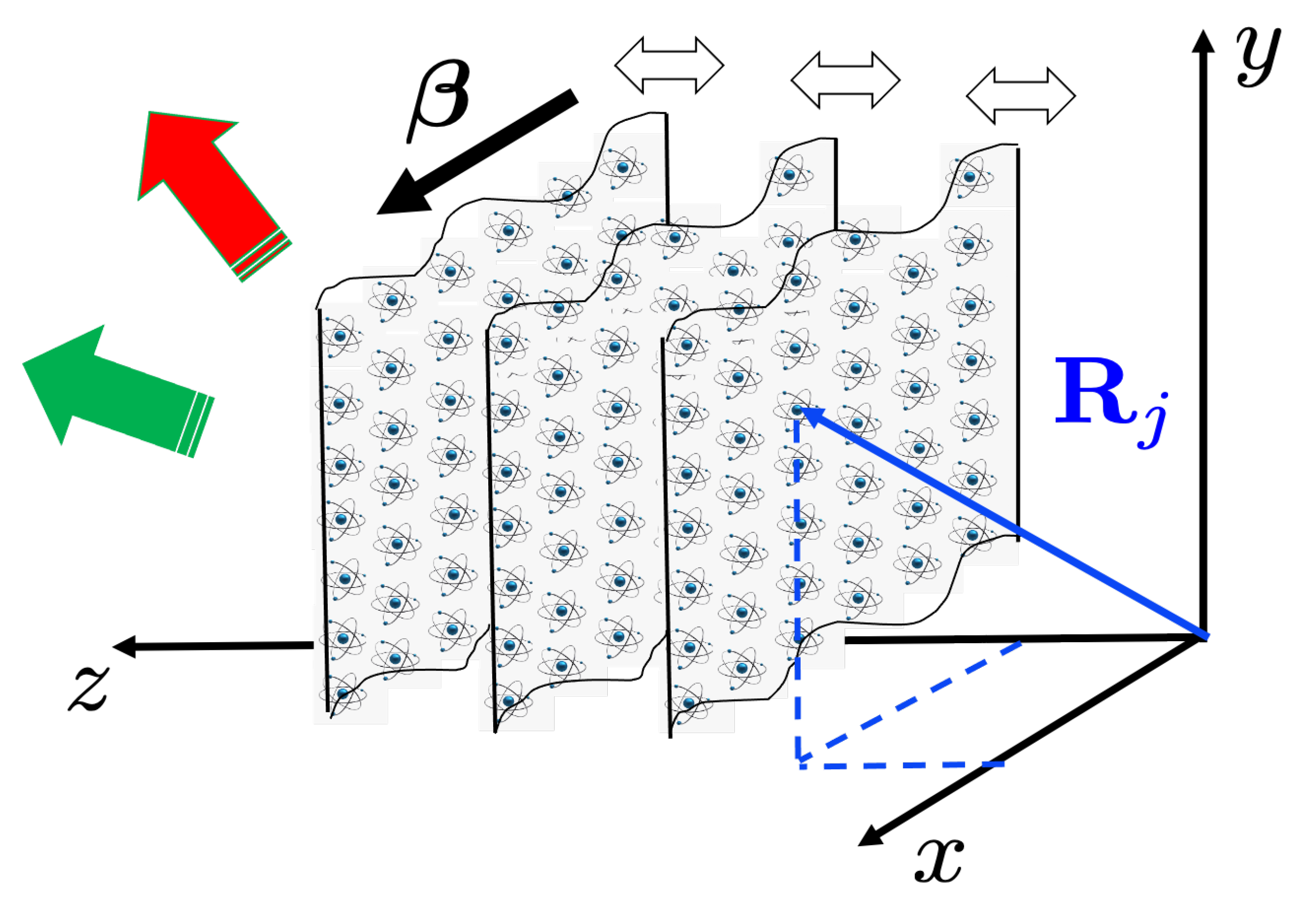Figure 2 shows how the momentum kick controls the directionality of the emitted DCE pairs. In the figure, the emission direction of one of the photons is fixed vertical (${\mathbf{k}}_2=0$) and we trace over its polarization state. The emission lobes of the other photon are plotted for different values of $\mathit{\beta }$. For each $\mathit{\beta }$, maximal emission is when ${\mathbf{k}}_1=\mathit{\beta }$. The emission rate for TM photons is always larger than that for TE photons.

For an infinite atomic array in the $xy$-plane and finite along the z direction, i.e., mimicking a finite-width infinite-area slab, one can calculate the summation over in-plane atomic positions taking advantage of periodicity. In this case, we used the lattice summation identity

$$|\sum _j{e}^{i({\mathbf{k}}_1+{\mathbf{k}}_2-\mathit{\beta })·{\mathbf{r}}_j}{|}^2= {\left(2\pi \right)}^{2}A{n}_S^2\sum _{\mathbf{q}}\delta ({\mathbf{k}}_1+{\mathbf{k}}_2-\mathit{\beta }+\mathbf{q}),$$

(13)

where the sum over $\mathbf{q}$ corresponds to reciprocal momenta. Here, A is the (infinite) area of the slab and $n_S=N_x{N}_y/A=1/d^2$ is the number surface density of atoms. When all relevant wavelengths are much larger than the inter-atomic distance d, one can take the continuous limit approximation in which only $\mathbf{q}=0$ survives the sum over $\mathbf{q}$. Non-zero values of the reciprocal momentum correspond to high-order diffraction modes that are evanescent and do not contribute to the generation of DCE photons. Then, we obtained the in-plane linear momentum conservation condition:

$${\mathbf{k}}_1+{\mathbf{k}}_2=\mathit{\beta }.$$

(14)

The time-evolved quantum state can be written as

$$|{\psi }^{\left(\mathit{\beta }\right)}\left(t\right)\rangle =\sum _{\mathbf{k}}{\int }_0^{\mathsf{\Omega }}d\omega c_{\omega ,\mathbf{k}}^{\left(\mathit{\beta }\right)}\left(t\right)|\omega ,\mathsf{\Omega }-\omega \rangle \otimes |\mathbf{k},\mathit{\beta }-\mathbf{k}\rangle ,$$

(15)

and corresponds to a frequency-linear momentum entangled superposition.

In the absence of kick ($\mathit{\beta }=0$), the angular spectrum of the emitted photons is always symmetric with respect to the normal of the slab, ${\mathbf{k}}_1=-{\mathbf{k}}_2$, which is what happens in the standard DCE problem of a rigidly oscillating mirror [10]. In stark contrast, when $\mathit{\beta }\ne 0$, the traveling-wave modulation generates directed ripples on the mirror and produces photons that are emitted asymmetrically. This steered DCE emission can be interpreted as a modulation-induced asymmetry of the quantum vacuum.

The DCE emission rate is obtained by integrating out one of the photons in the emitted pair, $r_{{\mathbf{K}}_1,{\lambda }_1}^{\left(\mathit{\beta }\right)}={\sum }_{{\lambda }_2}\int d{\mathbf{K}}_2{r}_{{\mathbf{K}}_1,{\lambda }_1;{\mathbf{K}}_2,{\lambda }_2}^{\left(\mathit{\beta }\right)}$. For the finite-width infinite-area atomic array, the in-plane momentum ${\mathbf{k}}_2$ is fixed by the momentum conservation condition ${\mathbf{k}}_2=\mathit{\beta }-{\mathbf{k}}_1$, and the out-of-plane momentum is also fixed by the dispersion relation and the energy conservation condition, $k_{2z}={\zeta }_2[{(\mathsf{\Omega }-{\omega }_1)}^2/c^2-|\mathit{\beta }-{\mathbf{k}}_1{{|}^2]}^{1/2}$, where ${\zeta }_2=\pm 1$ gives the two possible emission directions normal to the array. Hence, the momentum integration above can be performed straightforwardly and only the summation over polarization states remains. Note that propagative DCE photons can be emitted only when $k_{1z}={\zeta }_1({\omega }_1^2/c^2-|{\mathbf{k}}_1{{|}^2)}^{1/2}$ and $k_{2z}$ are real. The spectral photon emission rate for photons with polarization ${\lambda }_1$, in-plane momentum in the interval $({\mathbf{k}}_1,{\mathbf{k}}_1+d{\mathbf{k}}_1)$, out-of-plane direction ${\zeta }_1$, and frequency in the interval $({\omega }_1,{\omega }_1+d{\omega }_1)$ takes the form

$$\frac{d{\mathsf{\Gamma }}_{{\zeta }_1,{\lambda }_1}^{\left(\mathit{\beta }\right)}({\mathbf{k}}_1,{\omega }_1)}{d{\mathbf{k}}_{1}d{\omega }_1}=\frac{{\omega }_1{r}_{{\mathbf{K}}_1,{\lambda }_1}^{\left(\mathit{\beta }\right)}}{c^2\left|k_{1z}\right|}=\frac{A{n}_S^2{\alpha }_0^2{\Delta }^2{\mathsf{\Omega }}^4{\omega }_1}{16{\left(2\pi \right)}^3{c}^5\left|k_{1z}\right|}{f}_{{\zeta }_1,{\lambda }_1}^{\left(\mathit{\beta }\right)}({\mathbf{k}}_1,{\omega }_1),$$

(16)

where

$$\begin{array}{c}\hfill f_{{\zeta }_1,{\lambda }_1}^{\left(\mathit{\beta }\right)}({\mathbf{k}}_1,{\omega }_1)=\frac{{\omega }_1{(\mathsf{\Omega }-{\omega }_1)}^2}{{\mathsf{\Omega }}^{2}c\left|k_{2z}\right|}\sum _{{\zeta }_2,{\lambda }_2}{F}_2({\zeta }_1|k_{1z}|,{\zeta }_2|k_{2z}\left|\right){\tilde{W}}_{{\mathbf{K}}_1,{\lambda }_1;{\mathbf{K}}_2,{\lambda }_2}^2.\end{array}$$

(17)

We perform the calculations in the linear polarization basis. Emitted photon pairs can be co-polarized, i.e., both transverse electric (TE) or both transverse magnetic (TM), with ${\tilde{W}}_{{\mathbf{K}}_1,TM;{\mathbf{K}}_2,TM}^2>{\tilde{W}}_{{\mathbf{K}}_1,TE;{\mathbf{K}}_2,TE}^2$. In addition, they can also be cross-polarized, i.e., one TE and one TM, with the rate being proportional to

$${\tilde{W}}_{{\mathbf{K}}_1,TE;{\mathbf{K}}_2,TM}^2\sim {[\widehat{\mathbf{z}}·({\mathbf{k}}_1\times {\mathbf{k}}_2)]}^2.$$

(18)

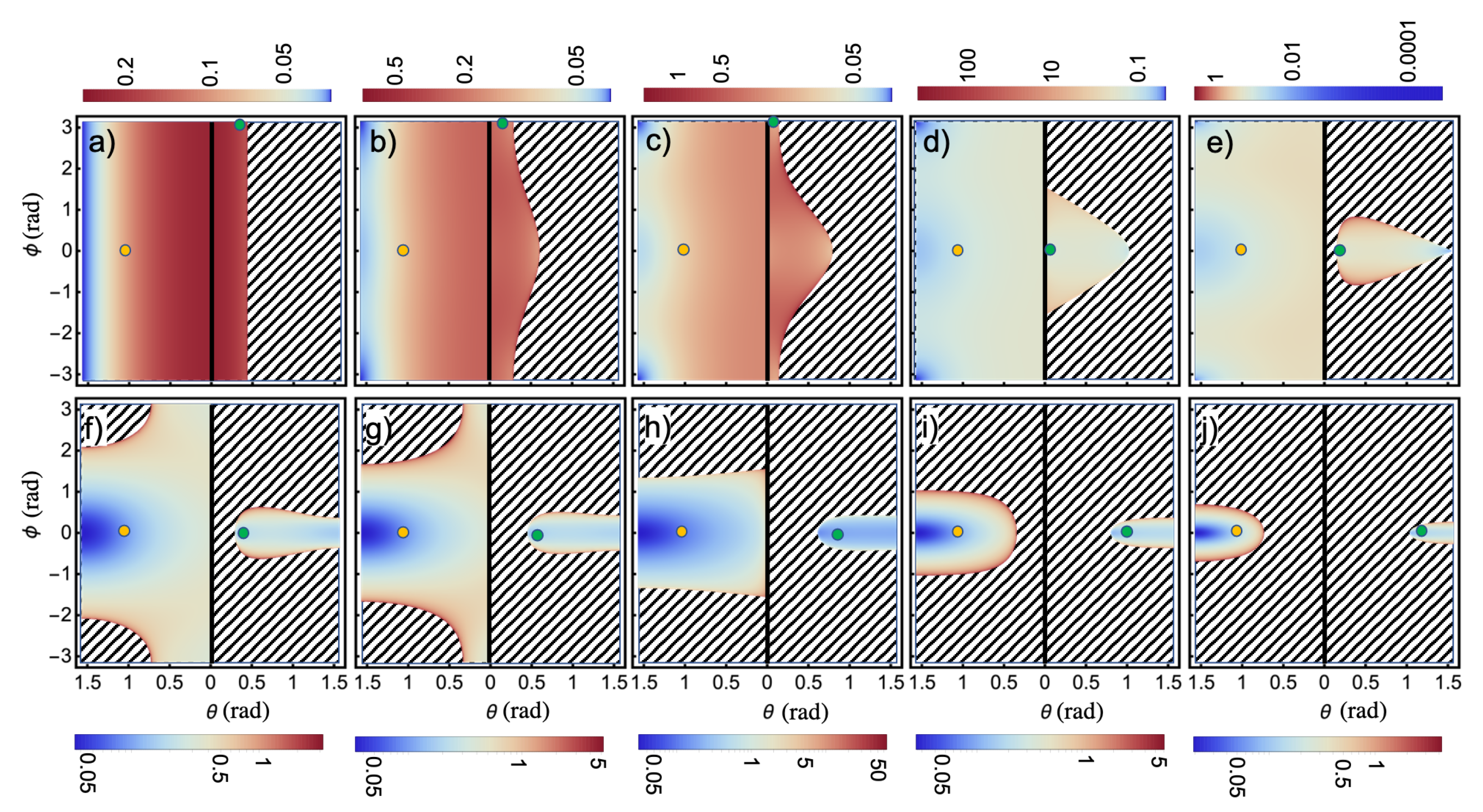
In the absence of momentum kick, the in-plane momenta of the photon pairs are collinear (${\mathbf{k}}_1=-{\mathbf{k}}_2$) and then cross-polarized emission is not possible. For non-zero momentum kick, the in-plane momenta are no longer collinear and cross-polarized emission is allowed. Figure 3 depicts $f_{\zeta ,\lambda }^{\left(\mathit{\beta }\right)}(\mathbf{k},\omega )$ for the case of an infinite monolayer, $\lambda =TE$ polarization and $\zeta =1$ (by symmetry, the plots for $\zeta =-1$ are identical). Polar density plots are shown both for the high-frequency (${\omega }_1>\mathsf{\Omega }/2$) and low-frequency (${\omega }_2<\mathsf{\Omega }/2$) photons in the emitted pair. In the absence of kick, there is rotational invariance along the azimuthal direction both for the high- and low-frequency photons. However, the former has a maximum polar angle of emission (panel a, area to the right of the central vertical solid line) while the latter can be emitted in any polar angle (panel a, area to the left of the central vertical solid line). The spherical emission profile (not shown, see [14]) for the low-frequency photon has a dome-like shape and for the high-frequency photon has a cone-like shape. As the magnitude of the momentum kick $\beta$ increases, the azimuthal rotational symmetry is broken and the distributions undergo intricate changes. The region of allowed emission for the high-frequency photon becomes deformed when the kick is non-zero, and at a critical value $c\beta =\mathsf{\Omega }-{\omega }_1$ (between panels d and e), an “island” of emission appears surrounded by a sea of forbidden emission directions (shaded areas). The island drifts to higher polar angles until it touches the grazing emission line when $c\beta =2{\omega }_1-\mathsf{\Omega }$ (between panels e and f). The island starts to shrink in size (panels f-j), and finally, at ${\beta }_{max}=\mathsf{\Omega }/c$, it collapses to a point (after panel j, not shown) and the photon is only emitted parallel to the kick. Far-field emission above that value of the kick is not possible. All of these plots can be interpreted in terms of the spherical emission profile: the cone at $\beta =0$ becomes tilted and deformed as $\mathit{\beta }$ increases. Regarding a low-frequency photon, its emission distribution remains mostly unperturbed until at $c\beta =\mathsf{\Omega }-2{\omega }_2$ two areas of forbidden emission appear at large polar angles and opposite to the kick direction (between panels e and f). The forbidden region grows until it engulfs its allowed emission region and a second island forms at $c\beta =\mathsf{\Omega }-{\omega }_2$ (between panels h and i). Finally, it ends up being emitted at a grazing angle but in a direction anti-parallel to the kick (after panel j, not shown). All of these plots can be interpreted in terms of the spherical emission profile: the dome at $\beta =0$ gets deformed as the momentum kick increases [14]. The modulation also excites hybrid entangled pairs composed of one photon and one evanescent surface wave (shaded areas), and when $\beta >{\beta }_{max}$, only evanescent modes are created on the atomic monolayer and subsequently decay via non-radiative loss mechanisms. At any given $\mathit{\beta }$, the maximal and minimal polar angles of emission for the high-frequency photon are ${\theta }_{1,max}\left(\beta \right)=\mathrm{Re}arcsin[(c\beta +\mathsf{\Omega })/{\omega }_1-1]$ and ${\theta }_{1,min}\left(\beta \right)=\max \{0,\mathrm{Re}arcsin[(c\beta -\mathsf{\Omega })/{\omega }_1+1]\}$. The low-frequency photon has a minimal polar angle of emission equal to ${\theta }_{2,min}\left(\beta \right)=\max \{0,\mathrm{Re}arcsin[(c\beta -\mathsf{\Omega })/{\omega }_1+1]\}$. 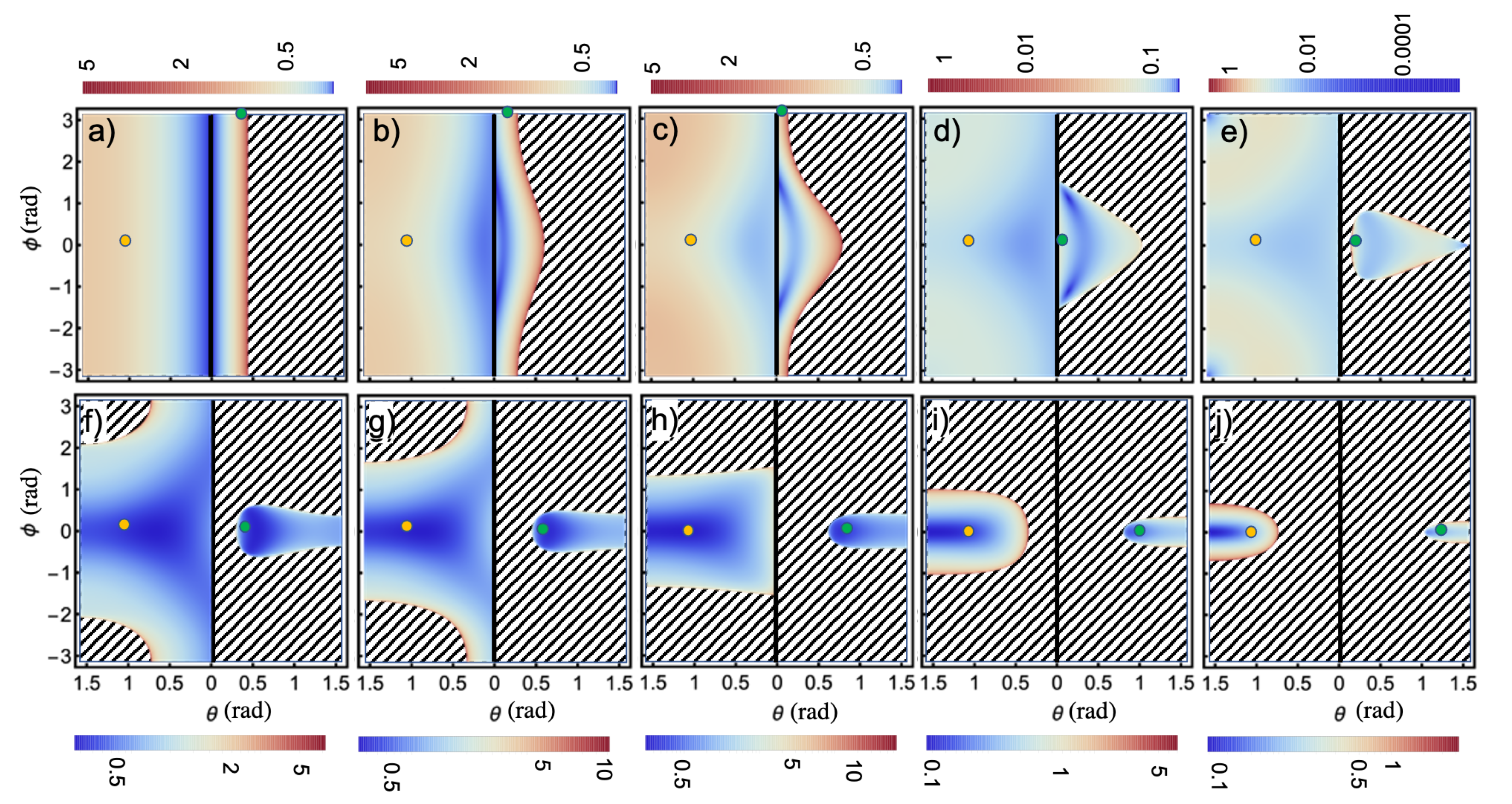Figure 4 shows the results for $\lambda =TM$ polarization. The overall structure of allowed and forbidden regions as a function of $\beta$ is identical to the TE case, with the maximal and minimal polar angles of emission given by the same expressions. There are, however, some distinct features in the shape of the angular emission spectrum at fixed $\mathit{\beta }$. The case $\beta =0$ has already been studied in [10]: For the low-frequency photon, emission is minimal at ${\theta }_2=0$ and gradually grows as the emission angle approaches the grazing direction, with the spherical emission profile having an inverted dome-like structure. For the high-frequency photon, emission is minimal at ${\theta }_1=0$, grows to a maximum as $\theta$ approaches $arcsin[\mathsf{\Omega }/{\omega }_1-1]$ (border of the cone), and then abruptly decays to zero for larger polar angles. As in the TE case, for $\mathit{\beta }>0$, the inverted dome and cone become deformed as the momentum kick increases.

In both the TE and TM cases, the emission directions of the two photons in a pair are correlated as

$$\begin{array}{c}\hfill {\omega }_{1}sin{\theta }_{1}sin{\phi }_1+{\omega }_{2}sin{\theta }_{2}sin{\phi }_2=0\\ \hfill {\omega }_{1}sin{\theta }_{1}cos{\phi }_1+{\omega }_{2}sin{\theta }_{2}cos{\phi }_2=c\beta .\end{array}$$

(19)

In the figures, we highlight two correlated emission directions for the low- and high-frequency photons, respectively, denoted as orange and green circles. The low-frequency photon is fixed at emission direction ${\phi }_2=0$, ${\theta }_2=\pi /3$, and the high-frequency photon is emitted at ${\phi }_1=\pi$ (anti-parallel to the kick) for $c\beta <{\omega }_{2}sin{\theta }_2$ and at ${\phi }_1=0$ (parallel to the kick) for $c\beta >{\omega }_{2}sin{\theta }_2$. Note that $\phi =\pm \pi$ are degenerate directions, and we only show the green circle at $\phi =\pi$ to avoid confusion.

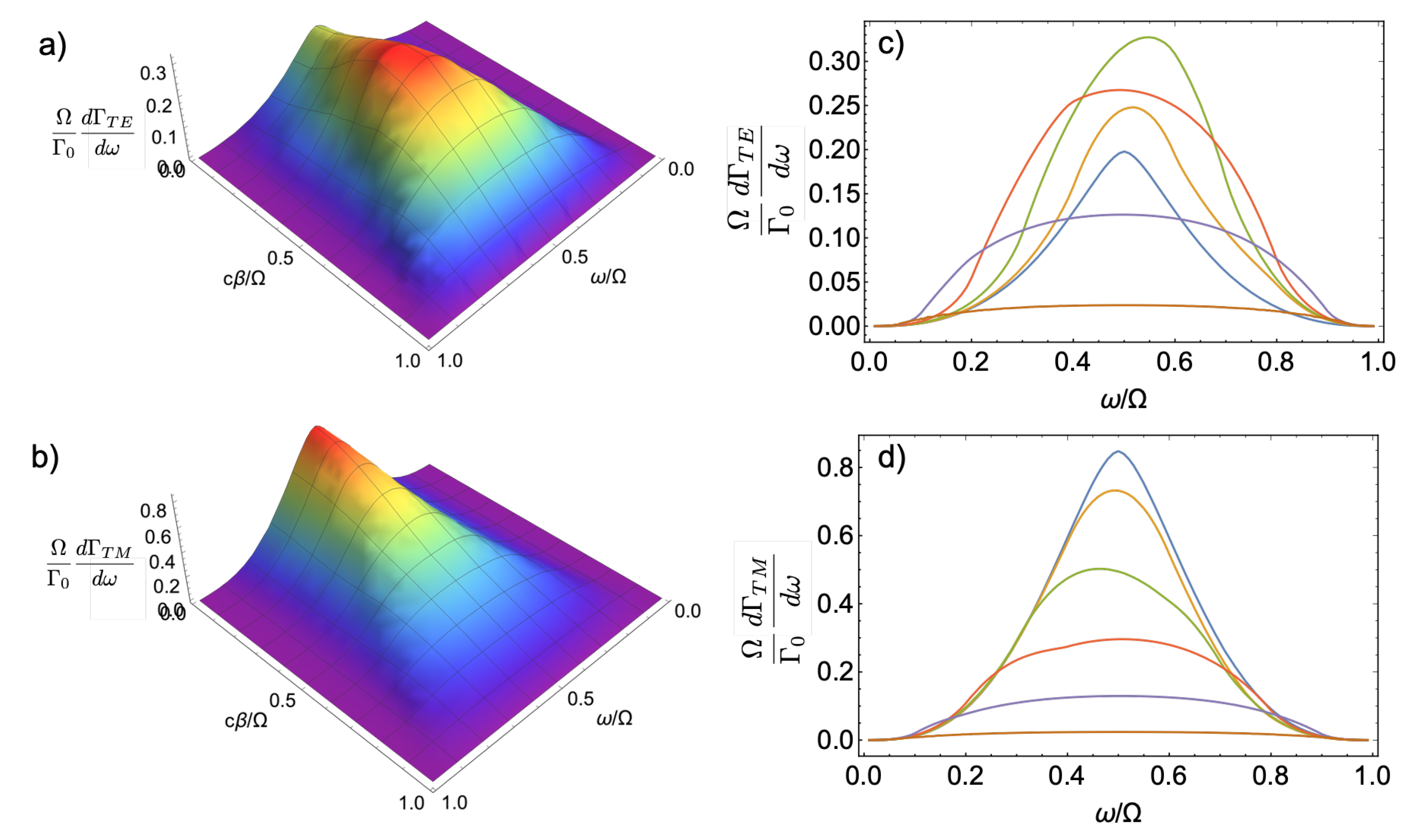
The DCE spectral emission rates for photons with polarization $\lambda$ are obtained by integrating over all emission directions

$$\frac{d{\mathsf{\Gamma }}_{\lambda }(\omega ,\beta )}{d\omega }=\frac{A{n}_S^2{\alpha }_0^2{\mathsf{\Omega }}^4{\Delta }^2}{16{\left(2\pi \right)}^3{c}^5}\sum _{\zeta }\int d\mathbf{k}\frac{\omega f_{\zeta ,\lambda }^{\left(\mathit{\beta }\right)}(\mathbf{k},\omega )}{|k_{1z}|}$$

(20)

and depends only on the modulus of the kick. The TE and TM spectral emission rates are shown in Figure 5 as a function of frequency and momentum kick. At zero momentum kick, they are both symmetric with respect to $\omega =\mathsf{\Omega }/2$ and the rate of TE emission is smaller than TM emission (note the different vertical scales in the plots). The two rates are identical to those derived in [10] for the standard DCE problem in the absence of synthetic phase. At non-zero kick, they both become slightly asymmetric, with the peak of the TE (TM) moving to frequencies larger (smaller) than $\omega =\mathsf{\Omega }/2$. The origin of the asymmetry is the non-zero cross-polarized emission. Indeed, the TE spectral emission rate has contributions from two terms, ${\tilde{W}}_{{\mathbf{K}}_1,TE;{\mathbf{K}}_2,TE}^2$ and ${\tilde{W}}_{{\mathbf{K}}_1,TE;{\mathbf{K}}_2,TM}^2$. The first term is symmetric around $\omega =\mathsf{\Omega }/2$ because, upon interchanging frequency, momentum, and spin indices, one gets ${\tilde{W}}_{{\mathbf{K}}_1,TE;{\mathbf{K}}_2,TE}^2={\tilde{W}}_{{\mathbf{K}}_2,TE;{\mathbf{K}}_1,TE}^2$. However, the second term is not symmetric because the same interchange gives ${\tilde{W}}_{{\mathbf{K}}_1,TE;{\mathbf{K}}_2,TM}^2={\tilde{W}}_{{\mathbf{K}}_2,TM;{\mathbf{K}}_1,TE}^2\ne {\tilde{W}}_{{\mathbf{K}}_2,TE;{\mathbf{K}}_1,TM}^2$. The same argument applies to the TM spectral emission rate. The spectral emission rate summed over polarizations is symmetric, though.

The total rate per polarization is obtained by integrating over frequency

$${\mathsf{\Gamma }}_{\lambda }\left(\beta \right)={\int }_0^{\mathsf{\Omega }}d\omega \frac{d{\mathsf{\Gamma }}_{\lambda }(\omega ,\beta )}{d\omega }.$$

(21)

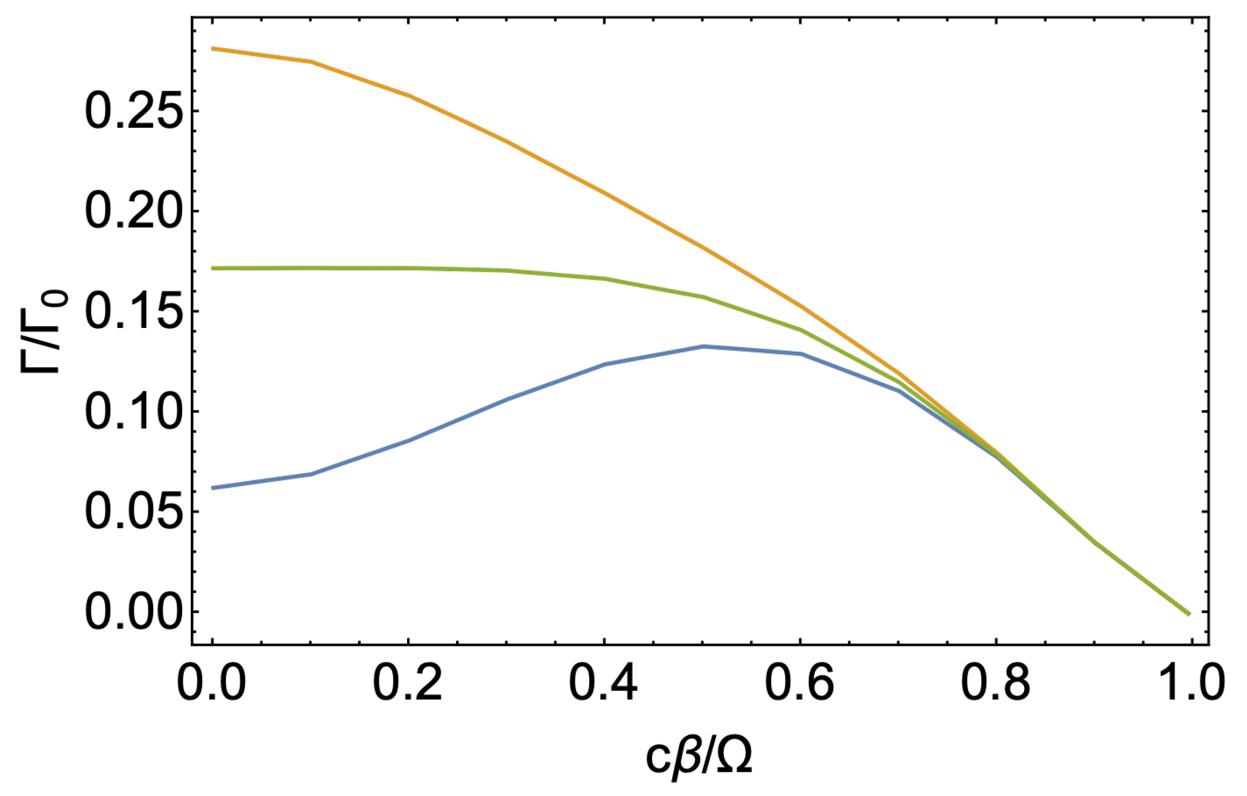
As shown in Figure 6, the TM rate has a monotonous decay to zero at ${\beta }_{max}=\mathsf{\Omega }/c$, while the TE rate decays non-monotonically. Furthermore, ${\mathsf{\Gamma }}_{TE}\left(\beta \right)<{\mathsf{\Gamma }}_{TM}\left(\beta \right)$ and their difference diminishes as the kick grows. The figure also shows the emission rate for circularly polarized photons, which is the same for right- and left-circular polarization, ${\mathsf{\Gamma }}_R\left(\beta \right)={\mathsf{\Gamma }}_L\left(\beta \right)$ and is initially flat and then decays monotonically to zero. As follows from the figure, ${\mathsf{\Gamma }}_{TE}\left(\beta \right)<{\mathsf{\Gamma }}_{R/L}\left(\beta \right)<{\mathsf{\Gamma }}_{TM}\left(\beta \right)$ and the total rate verify $\mathsf{\Gamma }\left(\beta \right)={\mathsf{\Gamma }}_{TE}\left(\beta \right)+{\mathsf{\Gamma }}_{TM}\left(\beta \right)=2{\mathsf{\Gamma }}_{R/L}\left(\beta \right)$.

3.2. Spinning Synthetic Phase

In this section we briefly discuss the case of a spinning synthetic phase $\mathsf{\Phi }\left(\mathbf{R}\right)=\ell \phi$. Due to the symmetry properties of the phase, one needs to quantize the electromagnetic field with angular momentum. Usually, this is performed in the paraxial approximation in terms of Laguerre–Gauss modes that carry orbital angular momentum [16]. However, for DCE, this is not appropriate because the emitted photon pairs are non-paraxial, and a more general approach is required. We follow the quantization scheme based on vector-Bessel modes that form a complete basis for the electromagnetic field with angular momentum and do not require any paraxial approximation [17]. In this scheme, neither orbital angular momentum (OAM) nor spin angular momentum (SAM) are good quantum numbers; only their sum is. Vector-Bessel modes are labelled by $\gamma =\{k,k_z,\eta ,m\}$, where $k\ge 0$ is the transverse linear momentum, $k_z$ is the axial linear momentum, $\eta =\pm 1$ is associated with the sign of the transverse spin $s_t=\pm \hslash c{k}_z/\omega$, and m is the total angular momentum (OAM plus SAM). The dispersion relation ${\omega }^2/c^2=k^2+k_z^2=K^2$ does not depend on m or $\eta$. In cylindrical coordinates, the vector-Bessel mode has the following components:

$$\begin{array}{ccc}\hfill E_{\rho }& =& \frac{i{e}^{i{k}_{z}z}{e}^{im\phi }}{\sqrt{2}\left(2\pi \right)}\left[\frac{k_z+\eta K}{2K}{J}_{m-1}\left(k\rho \right)-\frac{k_z-\eta K}{2K}{J}_{m+1}\left(k\rho \right)\right]\hfill \\ \hfill E_{\phi }& =& -\frac{e^{i{k}_{z}z}{e}^{im\phi }}{\sqrt{2}\left(2\pi \right)}\left[\frac{k_z+\eta K}{2K}{J}_{m-1}\left(k\rho \right)+\frac{k_z-\eta K}{2K}{J}_{m+1}\left(k\rho \right)\right]\hfill \\ \hfill E_z& =& \frac{e^{i{k}_{z}z}{e}^{im\phi }}{\sqrt{2}\left(2\pi \right)}\frac{k}{K}{J}_m\left(k\rho \right),\hfill \end{array}$$

(22)

where $J_m\left(x\right)$ are Bessel functions. Note that these modes are non-diffracting (constant amplitude along the z direction), have a topological vortex singularity along the z-axis for $m\ne 0$ with a phase wrapping equal to $2\pi m$, and decay along the radial direction.

The two-photon generation rate is

$$\begin{array}{c}\hfill r_{{\gamma }_1,{\gamma }_2}^{(\ell )}=\frac{\pi {\alpha }_0^2{\omega }_1{\omega }_2{\mathsf{\Omega }}^2{\Delta }^2}{8{\left(2\pi \right)}^2{c}^2}\delta ({\omega }_1+{\omega }_2-\mathsf{\Omega })\left|\sum _j{e}^{i(k_{1z}+k_{2z})z_j}{|}^2\right|\sum _j{T}_{{\gamma }_1,{\gamma }_2}\left({\rho }_j\right)e^{i(m_1+m_2-\ell ){\phi }_j}{|}^2,\end{array}$$

(23)

where we took the continuum limit ${\sum }_{k,k_z}\to V{\int }_{-\infty }^{\infty }d{k}_z{\int }_0^{\infty }kdk$. The function $T_{{\gamma }_1,{\gamma }_2}\left({\rho }_j\right)$ results from plugging the vector Bessel mode into Equation (9) and has a cumbersome expression that we do not write here (it is written below after performing the summation over j). Emitted photon pairs can have the same (${\eta }_1{\eta }_2=1$) or opposite (${\eta }_1{\eta }_2=-1$) signs of transverse spin. In contrast to the rate for the linear synthetic phase Equation (10), it is not possible to express the rate Equation (23) as that of a single atom multiplied by a multi-atom correction. The underlying reason is the nontrivial topology of the imprinted modulation, which is ill-defined for a single atom.

To perform the sum over atoms, we assume they are arranged into a cylindrical geometry of radius R and height $L_z$. The axis of the cylinder coincides with the axis of spinning modulation axis (z-direction). Equation (23) is the product of two array form factors: one is the same $F_2$ discussed in the previous section, and the other is a new $F_3$ that depends on all quantum numbers $k_1,k_2;k_{1z},k_{2z};{\eta }_1,{\eta }_2;m_1,m_2$ of the two photons. We compute $F_3$ in the continuum limit and replace the sum over atoms with an integral. Then,

$$\begin{array}{ccc}& & F_3={\left(2\pi \right)}^2{n}_S^2{\delta }_{m_1+m_2,\ell }{\left[{\int }_0^{R}drr{T}_{{\gamma }_1,{\gamma }_2}\left(r\right)\right]}^2,\hfill \end{array}$$

(24)

where $n_S$ is the number of atoms per unit of disk area. The spinning modulation generates vortex photon pairs for which the angular momentum must add up to the imprinted topological charge ℓ:

$$m_1+m_2=\ell$$

(25)

in agreement with angular momentum conservation. For $\ell =0$, the generated photons in a pair have opposite twist. The two-photon state is frequency-angular momentum entangled,

$$|{\psi }^{(\ell )}\left(t\right)\rangle =\sum _m{\int }_0^{\mathsf{\Omega }}d\omega c_{\omega ,m}^{(\ell )}\left(t\right)|\omega ,\mathsf{\Omega }-\omega \rangle \otimes |m,\ell -m\rangle .$$

(26)

The total emission rate from the modulated atomic array is

$${\mathsf{\Gamma }}_{\ell }=\frac{\pi {\alpha }_0^2{\mathsf{\Omega }}^2{\Delta }^2}{8{\left(2\pi \right)}^2{c}^6}{\int }_0^{\mathsf{\Omega }}d\omega {\omega }^2{(\mathsf{\Omega }-\omega )}^2{f}_{\ell }\left(\omega \right).$$

(27)

The spectral weight function $f_{\ell }\left(\omega \right)$ sums the product $F_2{F}_3$ over all degrees of freedom of the two photons except the frequency of one of them. In the case of zero imprinted angular momentum, the total rate is identical to that derived in [10] for the standard DCE problem: ${\mathsf{\Gamma }}_{\ell =0}={\mathsf{\Gamma }}_{\mathit{\beta }=0}={\mathsf{\Gamma }}_{\mathsf{\Phi }=0}$. To analyze the angular momentum content of the emitted radiation, we expand the spectral weight function into different m contributions, $f_{\ell }\left(\omega \right)=[{\pi }^2{n}_S^2{c}^4/{\omega }^2{(\mathsf{\Omega }-\omega )}^2]{\sum }_m{f}_{\ell }(\omega ,m)$. The angular momentum spectrum is

$$f_{\ell }(\omega ,m)={\int }_0^{u}d\kappa {\int }_0^{1-u}d{\kappa }^{\prime }\sum _{\zeta ,{\zeta }^{\prime }=\pm 1}\sum _{\eta ,{\eta }^{\prime }=\pm 1}{(t_a+t_b+t_c+t_d+t_e)}^2,$$

(28)

where the different terms are written in dimensionless variables $u=\omega /\mathsf{\Omega }$, ${\kappa }_z=\zeta {[u^2-{\kappa }^2]}^{1/2}$, and ${\kappa }_z^{\prime }={\zeta }^{\prime }{[{(1-u)}^2-{\left({\kappa }^{\prime }\right)}^2]}^{1/2}$, as

$$\begin{array}{ccc}\hfill t_a& =& [[{\kappa }_z+{\kappa }_z^{\prime }(1+{(1-u)}^{-1})]({\kappa }_z+\eta u)({\kappa }_z^{\prime }-{\eta }^{\prime }(1-u))\hfill \\ & & +\frac{{\left({\kappa }^{\prime }\right)}^2({\kappa }_z+\eta u)}{2(1-u)}+\frac{{\kappa }^2({\kappa }_z^{\prime }-{\eta }^{\prime }(1-u))}{2u}]{\mathcal{H}}_{m,\ell }^{(-)},\hfill \end{array}$$

(29)

$$\begin{array}{ccc}\hfill t_b& =& [[{\kappa }_z^{\prime }+{\kappa }_z(1+u^{-1})]({\kappa }_z^{\prime }+{\eta }^{\prime }(1-u))({\kappa }_z-\eta u)\hfill \\ & & +\frac{{\kappa }^2({\kappa }_z^{\prime }+{\eta }^{\prime }(1-u))}{2u}+\frac{{\left({\kappa }^{\prime }\right)}^2({\kappa }_z-\eta u)}{2(1-u)}]{\mathcal{H}}_{m,\ell }^{(+)},\hfill \end{array}$$

(30)

$$\begin{array}{ccc}\hfill t_c& =& \left[{\kappa }_z(2+u^{-1})+{\kappa }_z^{\prime }(2+{(1-u)}^{-1})\right]\kappa {\kappa }^{\prime }{\mathcal{H}}_{m,\ell }^{\left(0\right)},\hfill \end{array}$$

(31)

$$\begin{array}{ccc}\hfill t_d& =& -\left[\frac{{\left({\kappa }^{\prime }\right)}^2({\kappa }_z+\eta u)}{2(1-u)}+\frac{{\kappa }^2({\kappa }_z^{\prime }-{\eta }^{\prime }(1-u))}{2u}\right]{\mathcal{I}}_{m,\ell }^{(-)}\hfill \\ & & -\left[\frac{{\left({\kappa }^{\prime }\right)}^2({\kappa }_z-\eta u)}{2(1-u)}+\frac{{\kappa }^2({\kappa }_z^{\prime }+{\eta }^{\prime }(1-u))}{2u}\right]{\mathcal{I}}_{m,\ell }^{(+)},\hfill \end{array}$$

(32)

$$\begin{array}{ccc}\hfill t_e& =& \frac{m\kappa ({\kappa }_z^{\prime }+{\eta }^{\prime }(1-u))}{u}{\mathcal{J}}_{m,\ell }^{(-)}+\frac{m\kappa ({\kappa }_z^{\prime }-{\eta }^{\prime }(1-u))}{u}{\mathcal{J}}_{m,\ell }^{(+)}\hfill \\ & & +\frac{(\ell -m){\kappa }^{\prime }({\kappa }_z+\eta u)}{1-u}{\mathcal{K}}_{m,\ell }^{(-)}+\frac{(\ell -m){\kappa }^{\prime }({\kappa }_z-\eta u)}{1-u}{\mathcal{K}}_{m,\ell }^{(+)}.\hfill \end{array}$$

(33)

Here, we defined dimensionless integrals that are functions of $\kappa$, ${\kappa }^{\prime }$, and $\mathcal{R}=\mathsf{\Omega }R/c$:

$$\begin{array}{ccc}\hfill {\mathcal{H}}_{m,\ell }^{(\pm )}& =& -{(-1)}^{m-\ell }{\int }_0^{\mathcal{R}}dyy{J}_{m\pm 1}\left(\kappa y\right)J_{m\pm 1-\ell }\left({\kappa }^{\prime }y\right)\hfill \\ \hfill {\mathcal{H}}_{m,\ell }^{\left(0\right)}& =& {(-1)}^{m-\ell }{\int }_0^{\mathcal{R}}dyy{J}_m\left(\kappa y\right)J_{m-\ell }\left({\kappa }^{\prime }y\right)\hfill \\ \hfill {\mathcal{I}}_{m,\ell }^{(\pm )}& =& -{(-1)}^{m-\ell }{\int }_0^{\mathcal{R}}dyy{J}_{m\pm 1}\left(\kappa y\right)J_{m\mp 1-\ell }\left({\kappa }^{\prime }y\right)\hfill \\ \hfill {\mathcal{J}}_{m,\ell }^{(\pm )}& =& -{(-1)}^{m-\ell }{\int }_0^{\mathcal{R}}dy{J}_m\left(\kappa y\right)J_{m\mp 1-\ell }\left({\kappa }^{\prime }y\right)\hfill \\ \hfill {\mathcal{K}}_{m,\ell }^{(\pm )}& =& {(-1)}^{m-\ell }{\int }_0^{\mathcal{R}}dy{J}_{m\pm 1}\left(\kappa y\right)J_{m-\ell }\left({\kappa }^{\prime }y\right).\hfill \end{array}$$

(34)

For $\ell =0$, the integrals ${\mathcal{H}}^{(\pm )}$ and ${\mathcal{H}}^{\left(0\right)}$ are one of Lommel’s integrals and have a closed form, but the other three integrals do not. In the limit $\mathcal{R}\to \infty$, all of the integrals are of the Weber–Schafheitlin form, ${\int }_0^{\infty }dy{y}^q{J}_{\mu }\left(\kappa y\right)J_{\nu }\left({\kappa }^{\prime }y\right)$, with exponent $q=1$ or $q=0$. The above expressions allow us to calculate $f_{\ell }(\omega ,m)$ in space–time motion-induced DCE under spinning modulation. Direct inspection of $f_{\ell }(\omega ,m)$ shows that it satisfies the condition $f_{\ell }(\omega ,m)=f_{\ell }(\mathsf{\Omega }-\omega ,\ell -m)$. This identity states the simple fact that, as photons are emitted in pairs satisfying energy and angular momentum conservation, the emission rate of a photon with given frequency and angular momentum must be the same as the emission rate at the complementary frequency and angular momentum. In [14], we studied the angular momentum spectrum for DCE photons emitted from a quantum metasurface with spinning modulation of its optical properties. We numerically found that the angular momentum spectrum for the high-frequency photon $f_{\ell }({\omega }_1,m)$ is symmetric and maximal around the driving angular momentum ($m=\ell$) and that the one for the low-frequency photon $f_{\ell }({\omega }_2,m)$ is symmetric and maximal around the complementary angular momentum ($m=0$). The same properties are expected to occur for the case of space–time mechanical DCE.

Finally, we briefly discuss the structure of the energy density and Poynting vector in space–time DCE with spinning synthetic phase. Their expectation values on the evolved quantum state have a single vortex singularity along the z-axis for $\ell \ne 0$. The reason why there is a single vortex line is the non-diffracting nature of the vector-Bessel modes employed in the non-paraxial quantization scheme. Photons have well-defined projection of angular momentum along the z-axis and not with respect to their individual emission directions. Therefore, for $\ell \ne 0$, there is only one non-diffracting vortex line along the vertical direction and diffracting dual vortices do not occur.

4. Discussion

As mentioned in the Introduction, motional DCE involving temporal modulation of a boundary has not been observed to date because experimentally feasible mechanical modulation frequencies are insufficient for generating a large amount of photons. For example, the rate of photon creation from an oscillating perfectly reflecting mirror of area A is ${\mathsf{\Gamma }}_{DCE}=A{\mathsf{\Omega }}^5{\Delta }^2/15{\left(2\pi \right)}^2{c}^4$[18], which gives $\sim {10}^{-21}$ photons s${}^{-1}$ for a mirror of 1 cm${}^2$ area, modulation frequency $\mathsf{\Omega }/2\pi \sim$ 1 MHz, and modulation amplitude $\Delta \sim 100$ nm. An alternative approach to moving the whole mirror is to make its surface oscillate by launching acoustic waves, a scheme that is related to the proposed space–time motional DCE. However, usual materials can bear maximal relative deformations ${\delta }_{max}={\Delta }_{max}/(v_s/{\omega }_w)\sim {10}^{-2}$ ($v_s$ is the speed of sound, and ${\omega }_w$ is the frequency of the acoustic wave) and have maximal velocities of the boundary $v_{max}\sim {\delta }_{max}{v}_s\sim 50$ m/s, which again lead to negligibly small photo-production rates [2]. The same limitation occurs in space–time motional DCE. According to Figure 5, the maximal rate happens for zero synthetic phase and is

$${\mathsf{\Gamma }}_{max}\approx 0.34{\mathsf{\Gamma }}_0=\frac{0.34}{16{\left(2\pi \right)}^3}\frac{A{n}_S^2{\alpha }_0^2{\mathsf{\Omega }}^7{\Delta }^2}{c^6}.$$

(35)

We estimate it for experimentally feasible parameters of a spatiotemporally modulated meta-mirror consisting of an array of ${}^{87}$Rb atoms (ground state polarizability ${\alpha }_0=5.9\times {10}^{-28}{\mathrm{m}}^3$[19]) loaded into a 2D square optical lattice and vertically trapped by another shaking optical lattice. For a lattice constant $d=532$ nm, unit filling, $N\sim 200$ atoms ($A\sim 50$${\mathrm{m}}^2$, $n_S\sim 4$${\mathrm{m}}^{-2}$) [20], modulation amplitude $\Delta \sim 100$ nm, and modulation frequency $\mathsf{\Omega }/2\pi \sim 10$ kHz [21,22], the maximal rate is ${\mathsf{\Gamma }}_{max}\sim {10}^{-77}$ photons s${}^{-1}$. Again, unrealistic large modulation frequencies would be required to get measurable DCE rates.

In order to face these severe limitations of both standard and space–time motional DCE, analog DCE set-ups based on modulation of optical properties are required. For standard DCE, the experiment [6] based on a superconducting microwave coplanar waveguide is an analog of a one-dimensional DCE mirror, with the rate given by $\mathsf{\Gamma }=(\mathsf{\Omega }/12\pi ){(v_{eff}/c)}^2$, where $v_{eff}$ is the effective velocity of the mirror. For the experimental parameters $\mathsf{\Omega }/2\pi =11$ GHz and $v_{eff}/c=0.05$, the estimated rate is $\mathsf{\Gamma }\sim {10}^6$ photons s${}^{-1}$. For space–time DCE, a possible analog of a DCE mirror is a set-up consisting of a graphene-disk metasurface in which the electro-optical properties are spatiotemporally modulated and photon pairs are emitted into the full solid angle (as a three-dimensional DCE mirror). As shown in [14], all-optical modulation of the Fermi energy at THz frequencies enables giant rates $\mathsf{\Gamma }\sim {10}^{12}$ photons s${}^{-1}$ from centimeter-sized metasurfaces.

5. Conclusions

The space–time dynamical Casimir effect offers a novel degree of control over photo-production from the quantum vacuum. A space-dependent synthetic phase distribution imprinted on the temporal modulation protocol of optical properties or geometrical boundaries enables the generation of photon pairs with tailored spatial modes and entanglement properties. Travelling-wave modulations, such as parallel ripples propagating on the surface of a mirror, generate steered photon pairs that are frequency-path entangled. Spinning-wave modulations, such as twisting ripples on the mirror, produce vortex photon pairs featuring frequency-angular momentum entanglement. The synthetic phase can be reconfigured on-demand by changing the modulation protocol, allowing to modify the nature of entanglement between the generated photon pairs.

We end the paper with a conjecture. As discussed above, the synthetic phase distribution $\mathsf{\Phi }\left(\mathbf{r}\right)$ is imprinted onto space–time quantum metasurfaces via temporal delay of the modulation signal on different meta-atoms [14]. The meta-atoms can all have the same geometry, as the case of the atomic array meta-mirror, or the surface can even have no meta-atoms (unstructured), as is the case of a flat mirror. In both scenarios, the spatial profile of the emitted DCE photons is controlled by the synthetic phase imprinted by the modulation. On the other hand, a phase distribution $\mathsf{\Psi }\left(\mathbf{r}\right)$ can be imprinted onto a static surface by decorating it with meta-atoms with judiciously designed geometrical parameters, so-called gradient metasurfaces. For example, a blazed grating mirror or a meta-mirror with resonators of varying size. The phase distribution controls the spatial profile of light reflected from the static metasurface. An interesting question is as follows: What is the nature of DCE emission when such gradient metasurfaces are set in motion along a direction normal to the metasurface plane? We conjecture that, when $\mathsf{\Psi }\left(\mathbf{r}\right)=\mathsf{\Phi }\left(\mathbf{r}\right)$, the emitted Casimir light from the moving gradient metasurface has the same properties as the Casimir light generated by the space–time modulation on an unstructured surface. For example, the blazed grating mirror moving orthogonal to the grating plane should produce steered frequency-path entangled photon pairs, just as a flat mirror under a spatiotemporal modulation with a linear synthetic phase would. A test of this conjecture will require to calculate DCE emission from moving surfaces decorated with complex nanostructures, an overwhelmingly challenging analytical calculation and a very hard numerical task on its own. Were the conjecture proven to be correct, it would allow for a much simpler evaluation of DCE emissions from moving structured bodies by simply considering unstructured bodies modulated with the appropriate synthetic phase.

References

1. Moore, G.T. Quantum theory of electromagnetic field in a variable-length one-dimensional cavity. J. Math. Phys. 1970, 11, 2679. [Google Scholar] [CrossRef]
2. Dodonov, V.V. Current status of the dynamical Casimir effect. Phys. Scr. 2010, 82, 038105. [Google Scholar] [CrossRef] [Green Version]
3. Dalvit, D.A.R.; Neto, P.A.M.; Mazzitelli, F.D. Fluctuations, dissipation, and the dynamical Casimir effect. In Casimir Physics; Lecture Notes in Physics; Springer: Berlin/Heidelberg, Germany, 2011. [Google Scholar]
4. Nation, P.D.; Johansson, J.R.; Blencowe, M.P.; Nori, F. Colloquium: Stimulating uncertainty: Amplifying the quantum vacuum with superconducting circuits. Rev. Mod. Phys. 2012, 84, 1. [Google Scholar] [CrossRef] [Green Version]
5. Dodonov, V.V. Fifty Years of the Dynamical Casimir Effect. Physics 2020, 2, 7. [Google Scholar] [CrossRef] [Green Version]
6. Wilson, C.M.; Johansson, G.; Pourkabirian, A.; Simoen, M.; Johansson, J.R.; Duty, T.; Nori, F.; Delsing, P. Observation of the dynamical Casimir effect in a superconducting circuit. Nature 2011, 479, 376. [Google Scholar] [CrossRef] [PubMed]
7. Jaskula, J.-C.; Partridge, G.B.; Bonneau, M.; Lopes, R.; Ruaudel, J.; Boiron, D.; Westbrook, C.I. Acoustic Analog to the Dynamical Casimir Effect in a Bose-Einstein Condensate. Phys. Rev. Lett. 2012, 109, 220401. [Google Scholar] [CrossRef] [PubMed] [Green Version]
8. Lahteenmaki, P.; Paraoanu, G.S.; Hassel, J.; Hakonen, P.J. Dynamical Casimir effect in a Josephson metamaterial. Proc. Nat. Acad. Sci. USA 2013, 110, 4234–4238. [Google Scholar] [CrossRef] [Green Version]
9. Vezzoli, S.; Mussot, A.; Westerberg, N.; Kudlinski, A.; Saleh, H.D.; Prain, A.; Biancalana, F.; Lantz, E.; Faccio, D. Optical analogue of the dynamical Casimir effect in a dispersion-oscillating fibre. Commun. Phys. 2019, 2, 84. [Google Scholar] [CrossRef]
10. Souza, R.M.; Impens, F.; Neto, P.A.M. Microscopic dynamical Casimir effect. Phys. Rev. A 2018, 97, 032514. [Google Scholar] [CrossRef] [Green Version]
11. Milonni, P.W. The Quantum Vacuum; Academic Press: London, UK, 1994. [Google Scholar]
12. Barton, G. On van der Waals friction. II: Between atom and half-space. New J. Phys. 2010, 12, 113045. [Google Scholar] [CrossRef] [Green Version]
13. Intravaia, F.; Mkrtchian, V.E.; Buhmann, S.; Scheel, S.; Dalvit, D.A.R.; Henkel, C. Friction forces on atoms after acceleration. J. Phys. Condes. Matter 2015, 27, 214020. [Google Scholar] [CrossRef] [PubMed] [Green Version]
14. Kort-Kamp, W.J.M.; Azad, A.K.; Dalvit, D.A.R. Space-Time Quantum Metasurfaces. arXiv 2021, arXiv:2101.10433. [Google Scholar]
15. Bekenstein, R.; Pikovski, I.; Pichler, H.; Shahmoon, E.; Yelin, S.F.; Lukin, M.D. Quantum metasurfaces with atom arrays. Nat. Phys. 2020, 16, 676. [Google Scholar] [CrossRef] [Green Version]
16. Calvo, G.F.; Picón, A.; Bagan, E. Quantum field theory of photons with orbital angular momentum. Phys. Rev. A 2006, 73, 013805. [Google Scholar] [CrossRef] [Green Version]
17. Van Enk, S.J.; Nienhuis, G. Commutation rules and eigenvalues of spin and orbital angular momentum of radiation fields. J. Mod. Opt. 1994, 41, 963. [Google Scholar] [CrossRef]
18. Maia Neto, P.A. Vacuum radiation pressure on moving mirrors. J. Phys. A Math. Gen. 1994, 27, 2167. [Google Scholar] [CrossRef]
19. Steck, D.A. Rubidium 87 D Line Data. Available online: http://steck.us/alkalidata (accessed on 21 November 2019).
20. Rui, J.; Wei, D.; Rubio-Abadal, A.; Hollerith, S.; Zeiher, J.; Stamper-Kurn, D.M.; Gross, C.; Bloch, I. A subradiant optical mirror formed by a single structured atomic layer. Nature 2020, 583, 369. [Google Scholar] [CrossRef] [PubMed]
21. Lignier, H.; Sias, C.; Ciampini, D.; Singh, Y.; Zenesini, A.; Morsch, O.; Arimondo, E. Dynamical control of matter-wave tunneling in periodic potentials. Phys. Rev. Lett. 2007, 99, 220403. [Google Scholar] [CrossRef] [PubMed] [Green Version]
22. Parker, C.V.; Ha, L.-C.; Chin, C. Direct observation of effective ferromagnetic domains of cold atoms in a shaken optical lattice. Nat. Phys. 2013, 9, 769. [Google Scholar] [CrossRef] [Green Version]
Figure 1. Concept of space–time motion-induced DCE. An atomic array is externally driven by a spatiotemporal modulation of their center-of-mass coordinates. Atoms oscillate along the z-direction and are temporally dephased by a linear synthetic phase distribution Φ ( R ) = β x . The modulation produces a traveling wave of ripples moving along the x-direction. Pairs of photons (red and green arrows) are emitted with in-plane linear momentum adding up to the momentum kick β .
Universe 07 00189 g001
Figure 2. Two-photon angular emission. Emission lobes in the x z -plane of one of the DCE emitted photons with (a) TE and (b) TM polarization for various magnitudes of the momentum kick β = β x ^ , namely, c β / Ω = 0 (blue), ± 0.1 (red), ± 0.2 (orange), ± 0.3 (cyan), and ± 0.4 (purple). Solid (dashed) curves correspond to positive (negative) values of β . The other photon is assumed to be emitted along the z-direction, and we trace over its polarization degree of freedom. The parameters are N x = N y = 50 , N z = 1 , L x = L y = 20 c / Ω , and ω 1 = ω 2 = Ω / 2 . The emission rate is normalized to r 0 = N x 2 N y 2 N z 2 α 0 2 Ω 3 Δ 2 / 16 ( 2 π ) 3 c 2 .
Universe 07 00189 g002
Figure 3. Density polar plots of emitted radiation in TE polarization. The function f ζ , λ ( β ) ( k , ω ) is plotted for various amplitudes of the momentum kick c β / Ω , varying from 0 to 0.9 in steps of 0.1 (aj), respectively, for the infinite periodic monolayer. The angles φ and θ are the usual azimuthal and polar angles. The kick is along the in-plane ( θ = π / 2 ) direction φ = 0 . Emission is independent of ζ , i.e., emission towards z > 0 and z < 0 are identical. The areas to the right (left) of the central vertical solid line correspond to the emission of the high- (low-) frequency photon in a pair. Orange circles denote a given emission direction of the low-frequency photon, fixed in all panels to φ 2 = 0 and θ 2 = π / 3 . Green circles denote the correlated emission direction of the high-frequency photon, φ 1 ( β ) and θ 1 ( β ) . Shaded areas highlight regions of forbidden two-photon emission. The parameters are ω 1 / Ω = 0.7 and ω 2 / Ω = 0.3 .
Universe 07 00189 g003
Figure 4. Density polar plots of emitted radiation in TM polarization. Plots correspond to the same momentum kicks as in Figure 3. The shown correlated emission directions (orange and green circles), as well as employed parameters, are the same as in Figure 3.
Universe 07 00189 g004
Figure 5. Spectral emission rate of DCE photons versus frequency and momentum kick for (a) TE and (b) TM photons. Panels (c,d) show cuts of the spectrum for TE and TM polarizations, respectively, at fixed c β / Ω = 0 (blue), 0.2 (orange), 0.4 (green), 0.6 (red), 0.8 (purple), and 0.95 (brown). We assume a monolayer with in-plane periodic boundary conditions. The spectral rates are normalized to Γ 0 / Ω = A n S 2 α 0 2 Ω 6 Δ 2 / 16 ( 2 π ) 3 c 6 . For β = 0 , the spectra are symmetric with respect to ω / Ω = 0.5 .
Universe 07 00189 g005
Figure 6. Total photon creation rate for the system considered in Figure 4 for TE (blue), TM (orange), and circularly (green) polarized photons.
Universe 07 00189 g006
Publisher’s Note: MDPI stays neutral with regard to jurisdictional claims in published maps and institutional affiliations.