
An Overview of the MUSES Calculation Engine and How It Can Be Used to Describe Neutron Stars


Abstract
1. Introduction
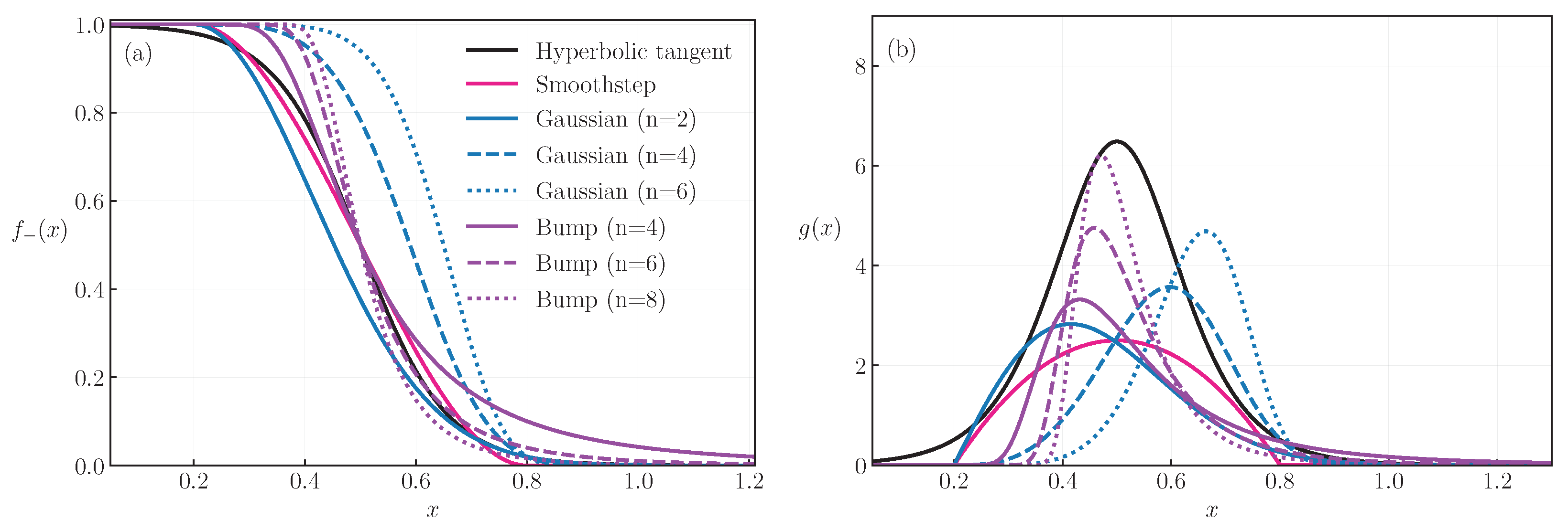
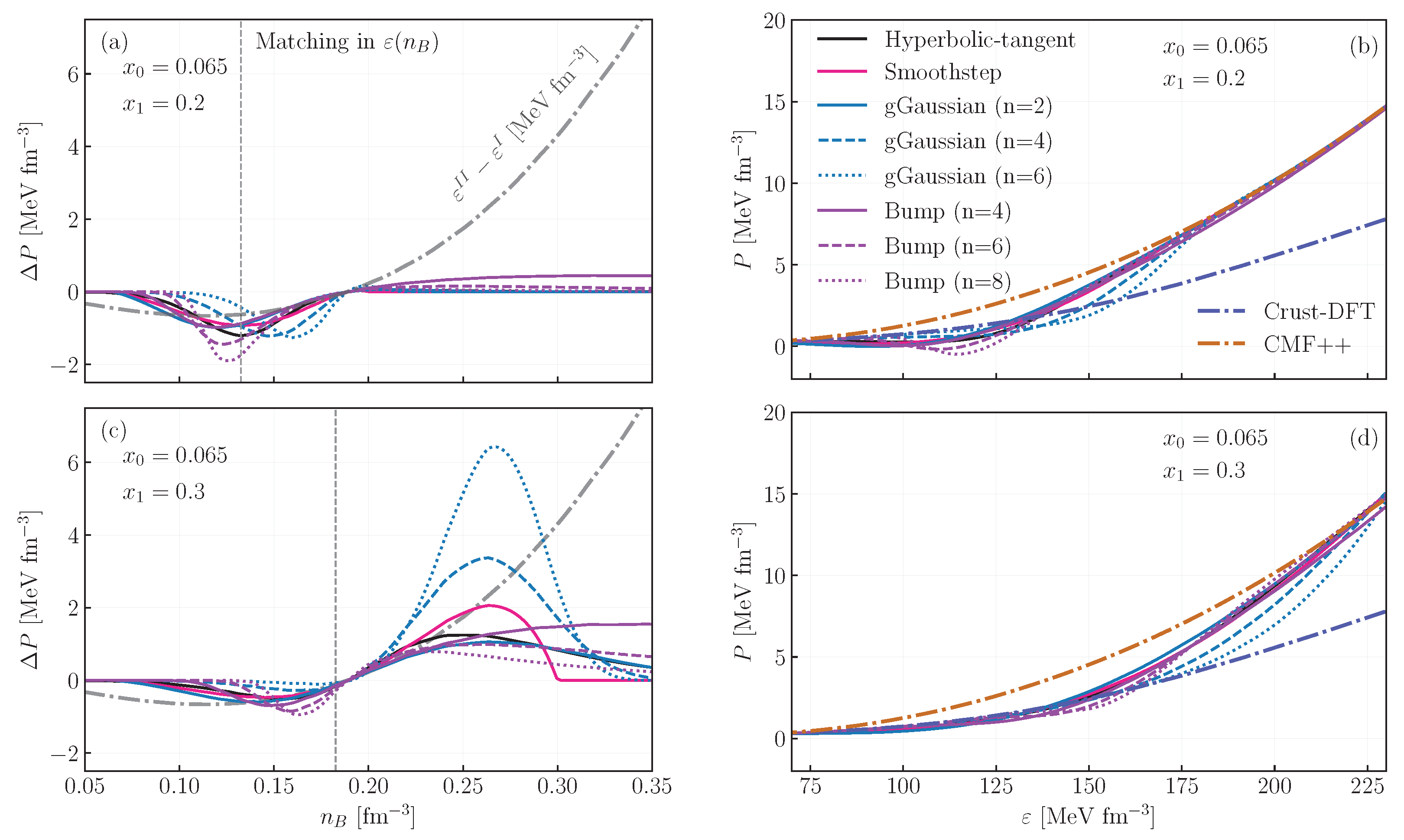
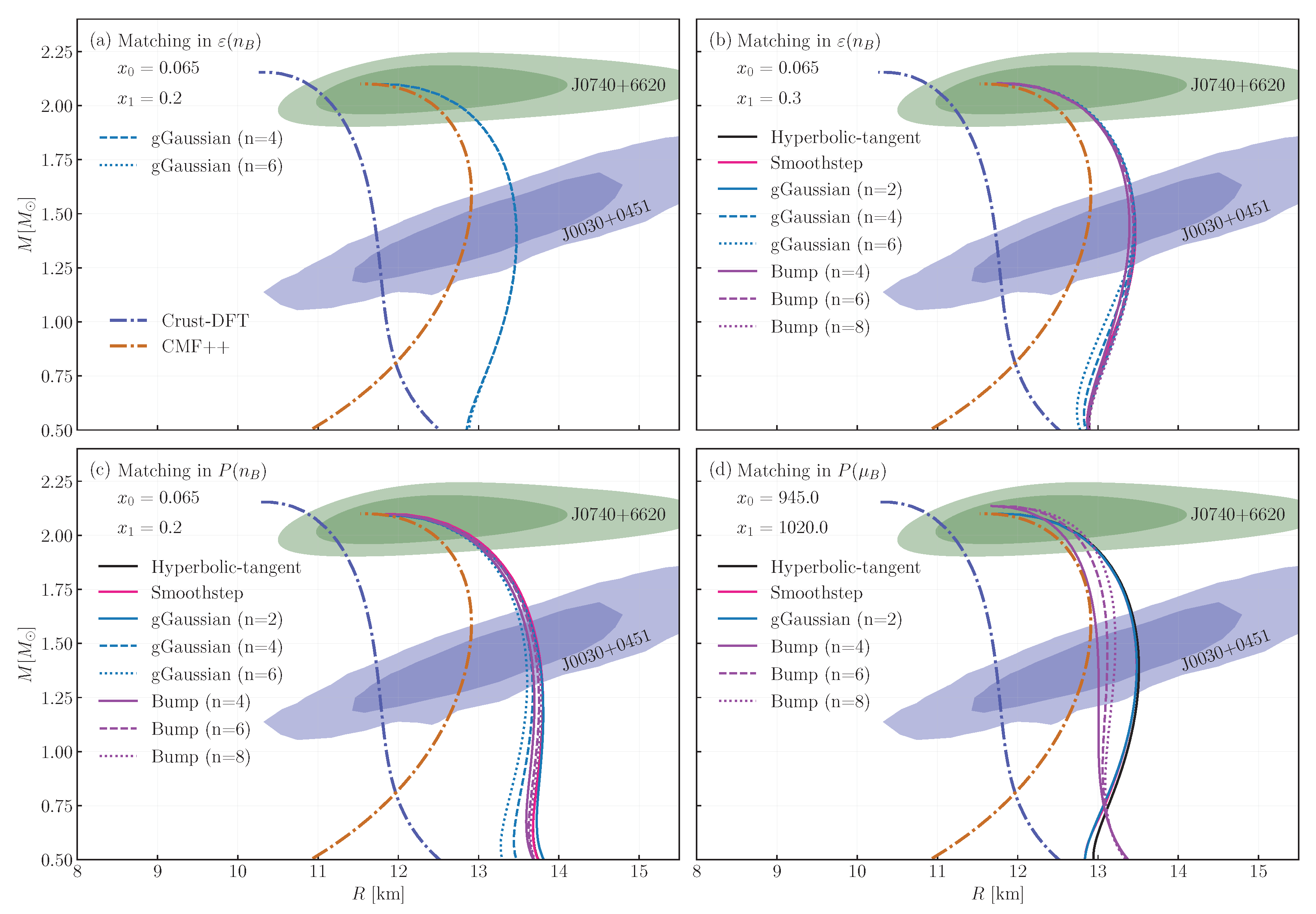
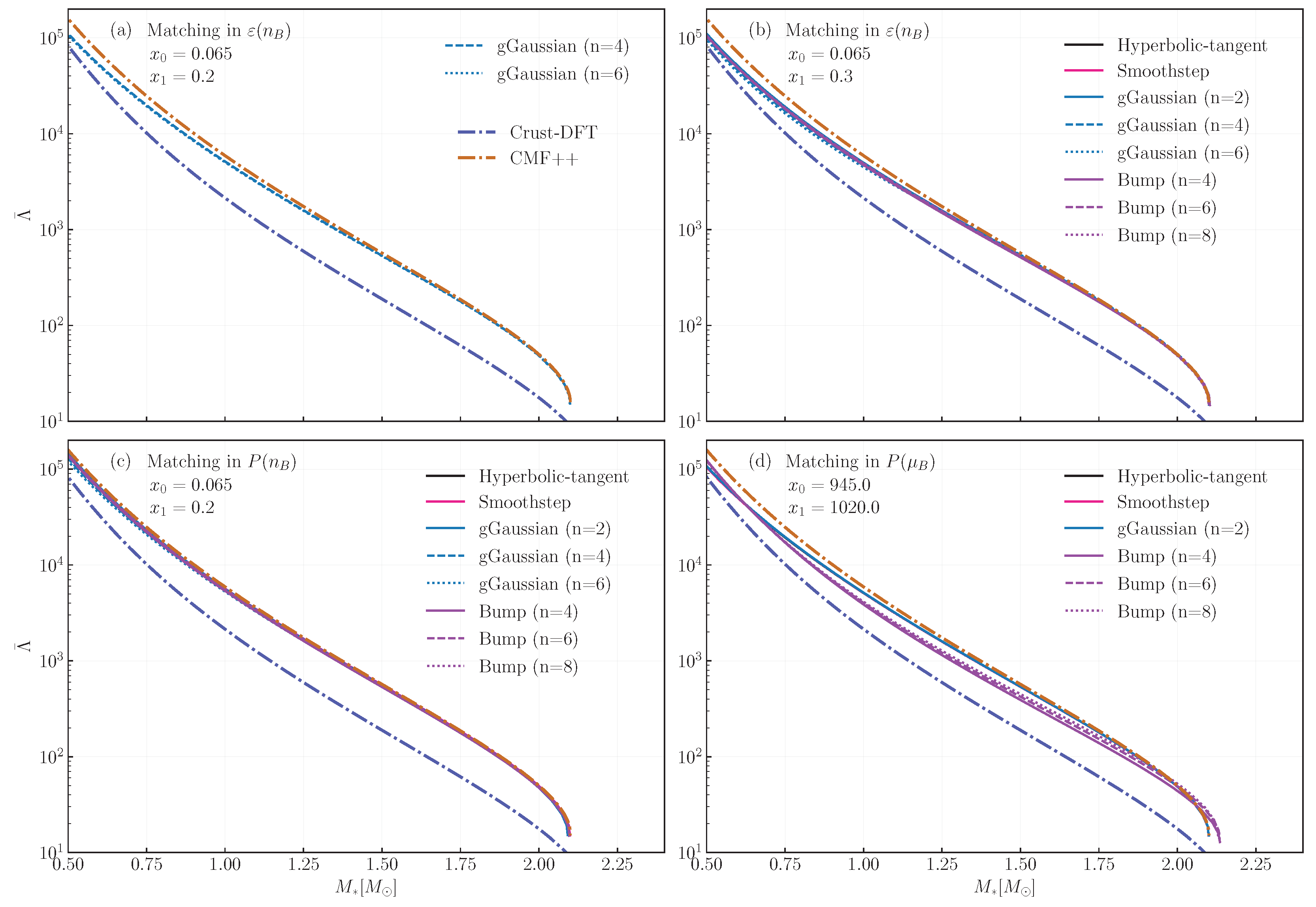
2. Formalism
- Hyperbolic tangent:
- Generalized Gaussian (gGaussian):
- Bump:
- Smoothstep:
3. Discussion and Conclusions
Author Contributions
Funding
Data Availability Statement
Acknowledgments
Conflicts of Interest
Abbreviations
| QCD | Quantum Chromodynamics |
| EoS | Equation of State |
| CE | Calculation Engine |
| MUSES | Modular Unified Solver of the Equation of State |
| CMF | Chiral Mean Field |
| DFT | Density Functional Theory |
| EFT | Chiral Effective Field Theory |
| TeExS | Ising 2D -Expansion Scheme |
| NumRelHol | Holographic EoS |
| QLIMR | Quadrupole-moment, Love-number, Moment of Inertia, Mass, and Radius |
Appendix A. Heavy-Ion Collisions
References
- Baym, G.; Hatsuda, T.; Kojo, T.; Powell, P.D.; Song, Y.; Takatsuka, T. From hadrons to quarks in neutron stars: A review. Rept. Prog. Phys. 2018, 81, 056902. [Google Scholar] [CrossRef]
- Harrison, B.K.; Thorn, K.S.; Wakano, M.; Wheeler, J.A. Gravitation Theory and Gravitational Collapse; University of Chicago Press: Chicago, IL, USA, 1965. [Google Scholar]
- Baym, G.; Pethick, C.; Sutherland, P. The Ground state of matter at high densities: Equation of state and stellar models. Astrophys. J. 1971, 170, 299–317. [Google Scholar] [CrossRef]
- Baym, G.; Pethick, C.; Pines, D. Superfluidity in Neutron Stars. Nature 1969, 224, 673–674. [Google Scholar] [CrossRef]
- Ivanenko, D.D.; Kurdgelaidze, D.F. Hypothesis concerning quark stars. Astrophysics 1965, 1, 251–252. [Google Scholar] [CrossRef]
- Ivanenko, D.; Kurdgelaidze, D.F. Remarks on quark stars. Lett. Nuovo Cim. 1969, 2, 13–16. [Google Scholar] [CrossRef]
- Collins, J.C.; Perry, M.J. Superdense Matter: Neutrons or Asymptotically Free Quarks? Phys. Rev. Lett. 1975, 34, 1353. [Google Scholar] [CrossRef]
- Kumar, R.; Dexheimer, V.; Jahan, J.; Noronha, J.; Noronha-Hostler, J.; Ratti, C.; Yunes, N.; Acuna, A.R.N.; Alford, M.; Anik, M.H.; et al. Theoretical and experimental constraints for the equation of state of dense and hot matter. Living Rev. Rel. 2024, 27, 3. [Google Scholar] [CrossRef]
- MUSES Project Website. 2024. Available online: https://musesframework.io/ (accessed on 16 June 2025).
- Du, X.; Steiner, A.W.; Holt, J.W. Hot and Dense Homogeneous Nucleonic Matter Constrained by Observations, Experiment, and Theory. Phys. Rev. C 2019, 99, 025803. [Google Scholar] [CrossRef]
- Du, X.; Steiner, A.W.; Holt, J.W. Hot and dense matter equation of state probability distributions for astrophysical simulations. Phys. Rev. C 2022, 105, 035803. [Google Scholar] [CrossRef]
- Steiner, A.; Roy, S. Crust-DFT Module v1.0.0. 2025. Available online: https://zenodo.org/records/14714273 (accessed on 16 June 2025).
- Machleidt, R.; Entem, D.R. Chiral effective field theory and nuclear forces. Phys. Rept. 2011, 503, 1–75. [Google Scholar] [CrossRef]
- Drischler, C.; Holt, J.W.; Wellenhofer, C. Chiral Effective Field Theory and the High-Density Nuclear Equation of State. Ann. Rev. Nucl. Part. Sci. 2021, 71, 403–432. [Google Scholar] [CrossRef]
- Friedenberg, D.; Holt, J.W. Chiral EFT Equation of State Module. 2024. Available online: https://zenodo.org/records/14611275 (accessed on 16 June 2025).
- Dexheimer, V.; Schramm, S. Proto-Neutron and Neutron Stars in a Chiral SU(3) Model. Astrophys. J. 2008, 683, 943–948. [Google Scholar] [CrossRef]
- Dexheimer, V.A.; Schramm, S. A Novel Approach to Model Hybrid Stars. Phys. Rev. C 2010, 81, 045201. [Google Scholar] [CrossRef]
- Cruz-Camacho, N.; Kumar, R.; Reinke Pelicer, M.; Peterson, J.; Manning, T.A.; Haas, R.; Dexheimer, V.; Noronha-Hostler, J. Phase Stability in the 3-Dimensional Open-source Code for the Chiral mean-field Model. arXiv 2024, arXiv:2409.06837. [Google Scholar] [CrossRef]
- Cruz Camacho, C.N.; Kumar, R.; Pelicer, M.; Manning, T.; Haas, R.; Dexheimer, V.; Noronha-Hostler, J. Chiral Mean Field Model (CMF++) Equation of State Module. 2025. Available online: https://zenodo.org/records/14860593 (accessed on 16 June 2025).
- Ravenhall, D.G.; Pethick, C.J. Neutron Star Moments of Inertia. Astrophys. J. 1994, 424, 846. [Google Scholar] [CrossRef]
- Bejger, M.; Haensel, P. Moments of inertia for neutron and strange stars: Limits derived for the Crab pulsar. Astron. Astrophys. 2002, 396, 917. [Google Scholar] [CrossRef]
- Yagi, K.; Stein, L.C.; Pappas, G.; Yunes, N.; Apostolatos, T.A. Why I-Love-Q: Explaining why universality emerges in compact objects. Phys. Rev. D 2014, 90, 063010. [Google Scholar] [CrossRef]
- Conde Ocazionez, C.A.; Tan, H.; Yunes, N. QLIMR Module. 2024. Available online: https://zenodo.org/records/14525356 (accessed on 16 June 2025).
- Alford, M.G.; Haber, A.; Zhang, Z. Isospin equilibration in neutron star mergers. Phys. Rev. C 2024, 109, 055803. [Google Scholar] [CrossRef]
- Alford, M.G.; Haber, A.; Zhang, Z. Beyond modified Urca: The nucleon width approximation for flavor-changing processes in dense matter. Phys. Rev. C 2024, 110, L052801. [Google Scholar] [CrossRef]
- Alford, M.; Zhang, Z. MUSES Flavor Equilibration Module. 2025. Available online: https://zenodo.org/records/14537518 (accessed on 16 June 2025).
- Reinke Pelicer, M.; Cruz-Camacho, N.; Conde, C.; Friedenberg, D.; Roy, S.; Zhang, Z.; Manning, T.A.; Alford, M.G.; Clevinger, A.; Grefa, J.; et al. Building neutron stars with the MUSES calculation engine. Phys. Rev. D 2025, 111, 103037. [Google Scholar] [CrossRef]
- Kambe, T.; Katayama, T.; Saito, K. Equation of State for Neutron Star Matter with NJL Model and Dirac–Brueckner–Hartree–Fock Approximation. JPS Conf. Proc. 2017, 14, 020807. [Google Scholar] [CrossRef]
- Wang, Q.W.; Shi, C.; Yan, Y.; Zong, H.S. Exploring hybrid star EOS with constraints from tidal deformability of GW170817. Nucl. Phys. A 2022, 1025, 122489. [Google Scholar] [CrossRef]
- Albright, M.; Kapusta, J.; Young, C. Baryon Number Fluctuations from a Crossover Equation of State Compared to Heavy-Ion Collision Measurements in the Beam Energy Range = 7.7 to 200 GeV. Phys. Rev. C 2015, 92, 044904. [Google Scholar] [CrossRef]
- Kapusta, J.I.; Welle, T.; Plumberg, C. Embedding a critical point in a hadron to quark-gluon crossover equation of state. Phys. Rev. C 2022, 106, 014909. [Google Scholar] [CrossRef]
- Salmi, T.; Choudhury, D.; Kini, Y.; Riley, T.; Vinciguerra, S.; Watts, A.L.; Wolff, M.T.; Arzoumanian, Z.; Bogdanov, S.; Chakrabarty, D.; et al. Data and Software for: ‘The Radius of the High-Mass Pulsar PSR J0740+6620 with 3.6 yr of NICER Data’. 2024. Available online: https://zenodo.org/records/10519473 (accessed on 29 May 2025).
- Salmi, T.; Choudhury, D.; Kini, Y.; Riley, T.E.; Vinciguerra, S.; Watts, A.L.; Wolff, M.T.; Arzoumanian, Z.; Bogdanov, S.; Chakrabarty, D.; et al. The Radius of the High-mass Pulsar PSR J0740+6620 with 3.6 yr of NICER Data. Astrophys. J. 2024, 974, 294. [Google Scholar] [CrossRef]
- Miller, M.C.; Lamb, F.K.; Dittmann, A.J.; Bogdanov, S.; Arzoumanian, Z.; Gendreau, K.C.; Guillot, S.; Harding, A.K.; Ho, W.C.G.; Lattimer, J.M.; et al. PSR J0030+0451 Mass and Radius from NICER Data and Implications for the Properties of Neutron Star Matter. Astrophys. J. Lett. 2019, 887, L24. [Google Scholar] [CrossRef]
- Miller, M.C.; Lamb, F.K.; Dittmann, A.J.; Bogdanov, S.; Arzoumanian, Z.; Gendreau, K.C.; Guillot, S.; Harding, A.K.; Ho, W.C.G.; Lattimer, J.M.; et al. NICER PSR J0030+0451 Illinois-Maryland MCMC Samples. 2019. Available online: https://zenodo.org/records/3473466 (accessed on 29 May 2025).
- Tan, H.; Noronha-Hostler, J.; Yunes, N. Neutron Star Equation of State in light of GW190814. Phys. Rev. Lett. 2020, 125, 261104. [Google Scholar] [CrossRef]
- Tan, H.; Dore, T.; Dexheimer, V.; Noronha-Hostler, J.; Yunes, N. Extreme matter meets extreme gravity: Ultraheavy neutron stars with phase transitions. Phys. Rev. D 2022, 105, 023018. [Google Scholar] [CrossRef]
- Tan, H.; Dexheimer, V.; Noronha-Hostler, J.; Yunes, N. Finding Structure in the Speed of Sound of Supranuclear Matter from Binary Love Relations. Phys. Rev. Lett. 2022, 128, 161101. [Google Scholar] [CrossRef]
- Boerner, T.J.; Deems, S.; Furlani, T.R.; Knuth, S.L.; Towns, J. ACCESS: Advancing Innovation: NSF’s Advanced Cyberinfrastructure Coordination Ecosystem: Services & Support. In Proceedings of the Practice and Experience in Advanced Research Computing 2023: Computing for the Common Good, New York, NY, USA, 23–27 July 2023; PEARC ’23. pp. 173–176. [Google Scholar] [CrossRef]
- Manning, T.A. MUSES Calculation Engine v1.0.0. 2025. Available online: https://zenodo.org/records/14721912 (accessed on 16 June 2025).
- ALICE Collaboration. Enhanced production of multi-strange hadrons in high-multiplicity proton-proton collisions. Nat. Phys. 2017, 13, 535–539. [Google Scholar] [CrossRef]
- Plumberg, C.; Almaalol, D.; Dore, T.; Mroczek, D.; Martín, J.S.S.; Serenone, W.M.; Spychalla, L.; Carzon, P.; Sievert, M.D.; Gardim, F.G.; et al. BSQ Conserved Charges in Relativistic Viscous Hydrodynamics solved with Smoothed Particle Hydrodynamics. arXiv 2024, arXiv:2405.09648. [Google Scholar]
- Gardim, F.G.; Almaalol, D.; Salinas San Martín, J.; Plumberg, C.; Noronha-Hostler, J. Unlocking “imprints” of conserved charges in the initial state of heavy-ion collisions. arXiv 2024, arXiv:2411.00590. [Google Scholar]
- Noronha-Hostler, J.; Parotto, P.; Ratti, C.; Stafford, J.M. Lattice-based equation of state at finite baryon number, electric charge and strangeness chemical potentials. Phys. Rev. C 2019, 100, 064910. [Google Scholar] [CrossRef]
- Jahan, J.; Shah, H.; Parotto, P.; Karthein, J.M.; Noronha-Hostler, J.; Ratti, C. 4D Taylor-Expanded Lattice (BQS) Module v1.0.0. 2025. Available online: https://zenodo.org/records/14639786 (accessed on 16 June 2025).
- Borsányi, S.; Fodor, Z.; Guenther, J.N.; Kara, R.; Katz, S.D.; Parotto, P.; Pásztor, A.; Ratti, C.; Szabó, K.K. Lattice QCD equation of state at finite chemical potential from an alternative expansion scheme. Phys. Rev. Lett. 2021, 126, 232001. [Google Scholar] [CrossRef]
- Kahangirwe, M.; Bass, S.A.; Bratkovskaya, E.; Jahan, J.; Moreau, P.; Parotto, P.; Price, D.; Ratti, C.; Soloveva, O.; Stephanov, M. Finite density QCD equation of state: Critical point and lattice-based T′ expansion. Phys. Rev. D 2024, 109, 094046. [Google Scholar] [CrossRef]
- Kahangirwe, M.; Jahan, J.; Parotto, P.; Stephanov, M.; Ratti, C. Ising 2D T′-Expansion Scheme (Ising-2DTExS) Module v1.0.0. 2025. Available online: https://zenodo.org/records/14637802 (accessed on 16 June 2025).
- Critelli, R.; Noronha, J.; Noronha-Hostler, J.; Portillo, I.; Ratti, C.; Rougemont, R. Critical point in the phase diagram of primordial quark-gluon matter from black hole physics. Phys. Rev. D 2017, 96, 096026. [Google Scholar] [CrossRef]
- Rougemont, R.; Grefa, J.; Hippert, M.; Noronha, J.; Noronha-Hostler, J.; Portillo, I.; Ratti, C. Hot QCD phase diagram from holographic Einstein–Maxwell–Dilaton models. Prog. Part. Nucl. Phys. 2024, 135, 104093. [Google Scholar] [CrossRef]
- Grefa, J.; Noronha, J.; Noronha-Hostler, J.; Portillo, I.; Ratti, C.; Rougemont, R. Hot and dense quark-gluon plasma thermodynamics from holographic black holes. Phys. Rev. D 2021, 104, 034002. [Google Scholar] [CrossRef]
- Hippert, M.; Grefa, J.; Manning, T.A.; Noronha, J.; Noronha-Hostler, J.; Portillo Vazquez, I.; Ratti, C.; Rougemont, R.; Trujillo, M. Bayesian location of the QCD critical point from a holographic perspective. Phys. Rev. D 2024, 110, 094006. [Google Scholar] [CrossRef]
- Yang, Y.; Hippert, M. Holographic Equation of State Module v1.0.0. 2025. Available online: https://zenodo.org/records/14695243 (accessed on 16 June 2025).
- Hippert, M.; Grefa, J.; Manning, T.A.; Noronha, J.; Noronha-Hostler, J.; Portillo Vazquez, I.; Ratti, C.; Rougemont, R.; Trujillo, M. Bayesian Analysis of the Equation of State of Quantum Chromodynamics from a Holographic Model. 2024. Available online: https://zenodo.org/records/13830379 (accessed on 16 June 2025).


| Function | Location of | Value of |
|---|---|---|
| Hyperbolic tangent | ||
| Gaussian | ||
| Bump | ||
| Smoothstep |
Disclaimer/Publisher’s Note: The statements, opinions and data contained in all publications are solely those of the individual author(s) and contributor(s) and not of MDPI and/or the editor(s). MDPI and/or the editor(s) disclaim responsibility for any injury to people or property resulting from any ideas, methods, instructions or products referred to in the content. |
© 2025 by the authors. Licensee MDPI, Basel, Switzerland. This article is an open access article distributed under the terms and conditions of the Creative Commons Attribution (CC BY) license (https://creativecommons.org/licenses/by/4.0/).
Share and Cite
Pelicer, M.R.; Dexheimer, V.; Grefa, J. An Overview of the MUSES Calculation Engine and How It Can Be Used to Describe Neutron Stars. Universe 2025, 11, 200. https://doi.org/10.3390/universe11070200
Pelicer MR, Dexheimer V, Grefa J. An Overview of the MUSES Calculation Engine and How It Can Be Used to Describe Neutron Stars. Universe. 2025; 11(7):200. https://doi.org/10.3390/universe11070200
Chicago/Turabian StylePelicer, Mateus Reinke, Veronica Dexheimer, and Joaquin Grefa. 2025. "An Overview of the MUSES Calculation Engine and How It Can Be Used to Describe Neutron Stars" Universe 11, no. 7: 200. https://doi.org/10.3390/universe11070200
APA StylePelicer, M. R., Dexheimer, V., & Grefa, J. (2025). An Overview of the MUSES Calculation Engine and How It Can Be Used to Describe Neutron Stars. Universe, 11(7), 200. https://doi.org/10.3390/universe11070200