Abstract
We performed a statistical study on the correlation between electromagnetic Ultra Low Frequency (ULF) waves and the evolution of relativistic electron fluxes in the outer radiation belt for during 101 geomagnetic storms that occurred between January 2013 and November 2018. We used the Van Allen Probes MagEIS and REPT instruments to study electron fluxes from 0.47 MeV to 5.2 MeV, and we utilized magnetic field data from EMFISIS to calculate magnetic field fluctuations parallel and perpendicular to the background magnetic field direction and obtain the ULF integrated power between 1 mHz and 10 mHz. We analyzed the data during the following three different time intervals: the main phase, the recovery phase, and the entire storm. We computed the Pearson’s correlation coefficient and mutual information score between the ratio of fluxes before and after each given phase and the total integrated ULF power during the same time interval. Our results show a significant correlation between ULF wave power and changes in fluxes of hundreds of keV electrons during the main phase of the storms and for MeV electrons during the recovery phase of the storms. By studying fluxes at independent , the largest correlations correspond to changes in fluxes before and after the entire storm and ULF fluctuations parallel to the field, especially for . We evaluated the drift resonance frequency for azimuthal wavenumber and found that for all considered energies and frequencies, the drift resonance with Pc5 ULF waves may occur in our region of study, which is consistent with the statistical results.
1. Introduction
The behavior of relativistic electrons in radiation belts is very dynamic. Electron fluxes in the outer radiation belt can undergo significant changes, varying by several orders of magnitude in minutes or hours due to interactions between the magnetosphere and the interplanetary medium. Relativistic electrons of MeV energies can cause damage to electronic circuits and components of space devices [1,2,3,4]. Thus, understanding the behavior of the radiation belts is important to prevent costly damage to infrastructure. This is especially relevant considering that satellites play a crucial role in communications, space weather, research, and others, and that the negative effects of relativistic electrons are exacerbated during geomagnetic storms [5]. Various physical processes play a fundamental role in electron evolution and variability as follows: geomagnetic activity [6,7,8,9]; the driver and type of a geomagnetic storm [9,10,11]; the altitude of the electron population in the radiation belts [12,13]; and the solar wind speed, density, and magnetic field [14,15,16,17], among others. Several efforts have been made to understand radiation belt dynamics, mostly using data measured by spacecraft missions, particularly during geomagnetic storms. The launch of the Van Allen Probes mission provided in situ information on radiation belts, as its orbits allowed us to obtain detailed data on parameters such as electron fluxes and wave energy at different radial distances near magnetic equatorial regions. These measurements have enabled researchers to analyze the evolution of radiation belt electrons due to different magnetospheric phenomena [7,18,19,20].
Outer radiation belt evolution is not easily predictable. Reeves et al. [6] found that the magnitude of the Dst index is not a determining factor for the evolution of electrons in the radiation belt, meaning that moderate or strong storms do not necessarily have a significant impact on the dynamics of relativistic electron fluxes. In addition, they found that 53% of geomagnetic storms result in an enhancement of relativistic electron fluxes in the outer radiation belt, 19% result in a depletion of the fluxes, and the remaining 28% of the storms produce no changes. More recently, Turner et al. [21], using data from the THEMIS mission, found that 58%, 25%, and 17% of storms result in enhancement, depletion, or no change, respectively. In addition, Zhao and Li [12], using data from the SAMPEX mission and considering the dependence, found that 40% of storms result in an enhancement, 40% result in no change, and 20% result in a depletion. Using data measured by the Van Allen Probes mission, Moya et al. [8] found similar statistical results and showed that the electron fluxes are distinct for different energies and during geomagnetic storms. Turner et al. [9] also studied this phenomenon and found that electron energies from tens of keV to MeV evolve differently during storms and that the impact of the driver varies during different storm phases. On the other hand, Zhao and Li [12] found that the Dst index and the speed of the solar wind do have an impact on the penetration of electrons into the radiation belt. Similarly, Kim et al. [16] found that a storm is not necessary for the electrons to evolve. Recent studies showed that the Auroral Electrojet (AE) index is, in fact, a better predictor of electron enhancement, regardless of the storm type [22,23,24]. Part of the complexity in understanding and predicting electron fluxes comes from the non-linear response of the belt to external drivers [25,26,27,28].
One factor that plays a fundamental role in the outer radiation belt variability corresponds to the waves that propagate through the magnetosphere. Indeed, wave-particle interactions can efficiently influence the dynamics of the plasma. Several studies have shown that wave processes are linked to the acceleration of particles in the radiation belt [29,30,31]. Simms et al. [32] showed that different electron populations are accelerated by their interaction with chorus waves. Elkington et al. [33] studied the process of drift resonance between ultra-low frequency (ULF) waves and relativistic electrons, and similarly, Mager and Klimushkin [34] studied the drift-bounce resonances with Alfvén waves. In this context, electromagnetic ULF waves in the frequency band between 1 mHz to 100 mHz are of great interest because they are relevant to the radiation belt dynamics [19,35]. The velocity of the solar wind can create perturbations in the magnetosphere when it interacts with the bow shock. This interaction can lead to various phenomena such as Kelvin-Helmholtz instabilities [36], shock-induced pulses in the magnetosphere [37], and others. These disturbances can cause continuous pulsations in the ULF Pc5 wave range, typically between 1.6 and 6.7 mHz [38]. ULF Pc5 waves generated during geomagnetic storms influence the ratio of electron fluxes between pre- and post-storm periods [6,39]. These waves can propagate and resonate with the particles of the radiation belt, in particular, with relativistic electrons [31,33,40,41,42,43]. Thus, the dynamic behavior of the radiation belt is partly controlled by ULF waves as radial diffusion can energize the electrons [44,45,46].
Different ULF wave modes, such as toroidal or poloidal relative to the Earth’s magnetic field, have different resonances and effects on particles at different energies and radial distances from the Earth [40,44,47]. Among the variety of electromagnetic waves that can be excited in the ULF range, the fundamental MHD modes correspond to the fast magnetosonic compressional mode and the transverse shear Alfvén mode [48]. These modes can interact and be coupled in the magnetosphere, for example, due to inhomogeneities or temperature effects [49], and have been found as field-aligned or transverse components of observed poloidal and toroidal ULF waves in the magnetosphere [42,50,51,52]. Despite this diversity of magnetospheric waves and modes, all ULF waves can be described as a superposition of perpendicular (transverse) and parallel (field-aligned) fluctuations, representing the shear Alfvén and the fast compressional modes, respectively. In this study, we investigate wave-particle interactions between relativistic electrons and ULF Pc5 waves in the outer radiation belt. We use measurements of electrons with energies between 470 keV and 5.2 MeV, within the range of , obtained from NASA’s Van Allen Probes data. In Section 2, we present a quick overview of the drift-bounce resonance theory. Section 3, describes the dataset and methodology. In Section 4, we analyze the relationship between the evolution of electron fluxes in the outer radiation belt and the ULF power for different phases of geomagnetic storms. Finally, in Section 5 we summarize and discuss our main results.
2. Theoretical Background: The Drift-Bounce Resonance
Multiple studies have shown that electrons and ULF waves can undergo resonant wave-particle interactions [33,40,53]. In the case of ULF waves with frequencies between 1 mHz and 10 mHz and relativistic electrons (with drift periods of around 3–10 min for relativistic and ultra-relativistic energies), the most relevant interaction is the drift-bounce resonance. Thus, using the drift-bounce resonance condition [53,54,55] we are able to identify what wave frequencies resonate with relativistic electrons at different energy levels. In particular, the drift-bounce resonance condition satisfies the following:
where is the wave angular frequency, is the east-west particle’s bounce-averaged drift rate, and m is the azimuthal wavenumber. Furthermore, is the particle’s bounce frequency, and N is the number of azimuthal wavelengths the particle drifts in a bounce cycle. Following Zhu et al. [53], averaging in equatorial pitch angle between 0 and 180°, the particle’s bounce-averaged drift rate is given by
with W and q, the relativistic energy and the charge of the electron, respectively. is calculated from the third adiabatic invariant, is the magnetic field on the Earth’s surface, and is the Earth’s radius.
In the case of relativistic electrons, the drift period is in the order of minutes, while the particle’s bounce motion is a few seconds long. Thus, the resonance between these particles and ULF waves in the Pc5 range is dominated by the drift motion [56], and the bounce motion may be neglected [53]. Therefore, for simplicity, and following previous works [33,47,54,55], in Equation (1), we only considered the drift resonance (). Regarding the value of the azimuthal wavenumber, m, perturbations in the azimuthal mode are traditionally associated with toroidal waves with low values for m [57]. Indeed, Balasis et al. [58] and Elkington et al. [41] have shown that the most important resonant interactions occur for . In particular, they observed that is dominant during the recovery phase, and and are present during the main phase of geomagnetic storms. These results are consistent with those obtained by Murphy et al. [47]. Thus, here we considered m-values between 1 and 10, which correspond to the dominant modulation for Pc5 waves, relevant for relativistic electrons [43,56]. Finally, it is relevant to mention that most of the approximations used here correspond to 1D or 2D approximations, and it has been shown that when 3D modeling ULF waves, the resonant conditions can be different [59].
3. Instrumentation and Data Analysis
We have analyzed the outer radiation belt using in situ data from the Van Allen Probes mission [60]. First, using the SYM-H data obtained from the OMNIWeb dataset, we selected 101 geomagnetic storm events between January 2013 and November 2018. We applied a similar criterion to that described in Moya et al. [8], selecting events where the SYM-H index was less than −50 nT. Then, the start of a storm is defined by the sharp increase in the SYM-H index, characteristic of the commencement of a sudden storm, or by the first noticeable drop in SYM-H. The recovery phase starts after the SYM-H minimum and ends when the SYM-H has recovered by 80%. A complete list of the geomagnetic storms can be found in the Supplementary Material. Electron data were obtained from the Relativistic Electron-Proton Telescope (REPT) [61] and Magnetic Electron Ion Spectrometer (MagEIS) [62] instruments of the Energetic Particle, Composition, and Thermal Plasma (ECT) suite [63] (https://spdf.gsfc.nasa.gov/pub/data/rbsp, accessed on 1 March 2024). Here we use electron fluxes between 470 keV and 1728 keV from MagEIS (Release 3) and between 1.8 MeV and 5.2 MeV from the REPT (Release 4) instrument. The electron fluxes were processed similarly for both MagEIS and ECT-REPT. The 11-s temporal resolution data were averaged over all pitch angles for fourteen energy channels between 470 keV and 5.2 MeV. We create a pitch angle-averaged flux function J, given by , with E being the energy of the electrons, t the time, and the pitch angle. We use orbital segments in the outer radiation belt for . An example of the satellite’s orbit and the flux of 1.8 MeV electrons along the trajectory of RBSP-A is shown in Figure 1b, for a geomagnetic storm that occurred on 27 February 2014. For each energy channel, the electron data were then binned with temporal and spatial scales of h and , respectively, where all the measurements inside each bin were averaged (linear values). The binning process aims to minimize the number of gaps in the data, and h was chosen because it produces gapless data up to consistently (for more information, see Moya et al. [8]). A figure showing how many data points are contained in each bin for a typical storm can be found in the Supplementary Material. In our calculations, corresponds to Roederer’s generalized L- shell parameter calculated using the OP77Q model and provided with the ECT data. The adopted corresponds to the Olson-Pfitzer model given for MagEIS and REPT data. Finally, to eliminate any possible non-physical effects from the satellites, the electron flux data with values below cm−2 s−1 sr−1 MeV−1 were eliminated for all energy channels. This elimination criterion follows Claudepierre et al. [64] and Moya et al. [8].
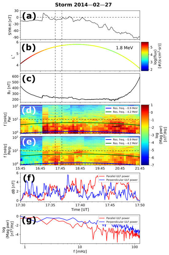
Figure 1.
Data obtained from the Van Allen Probes REPT and EMFISIS instruments for the geomagnetic storm of 27 February 2014. (a) SYM-H index. (b) Orbit of RBSP-A and electron flux for 1.8 MeV. (c) Magnetic field magnitude. (d) The magnetic ULF wave power with respect to fluctuations parallel to the background magnetic field. (e) Same as (d) but for perpendicular wave power. (f) Magnetic field fluctuations for a 20 min interval. (g) The PSD of magnetic field variations: parallel (blue) and perpendicular (orange) to the background field as a function of the frequency for the period shown in (f). The dashed black vertical lines indicate the 20 min time interval shown in panel (f), which was used to build the spectra shown in panel (g). Dashed black horizontal lines represent the range of wave frequency considered. The blue and green solid lines in panels (d,e) indicate the frequency of resonance with electrons of 0.9 MeV and 4.2 MeV, respectively.
The magnetic field data were obtained from the Electric and Magnetic Field Instrument Suite and Integrated Science (EMFISIS) [62,65] in Geocentric Solar Magnetospheric (GSM) coordinates. Figure 1c shows the magnitude of the magnetic field, , obtained from EMFISIS along the same trajectory shown in Figure 1b for RBSP-A. To investigate the effect of ULF waves on the evolution of relativistic electron fluxes, we computed the magnetic wave power in the range 1–10 mHz, which includes the Pc5 ULF waves frequency range. This analysis was conducted separately for parallel and perpendicular fluctuations with respect to the background magnetic field, as depicted in Figure 1d,e, respectively. The two horizontal dashed black lines in both panels indicate the frequency range of interest. To obtain the magnetic wave power, we first calculated the power spectral density matrices for parallel and perpendicular fluctuations, denoted as PSD‖ and PSD⊥, respectively. To construct these matrices, we consider the frequency where T is the wave period. To capture the ULF frequency spectrum from 1 mHz to 10 mHz, we selected time intervals of 1200 s for the magnetic field data obtained by EMFISIS, which has a time resolution of 4 s. This results in a frequency spectrum between 0.83 mHz and 125 mHz, with steps of 0.83 mHz. These 20 min magnetic field data intervals were shifted every 6 min to increase the total number of calculations. For each 20 min time series, we calculated the background magnetic field as , where the subscript i denotes the time step in the series. Subsequently, we determined the magnetic field variations as . The parallel and perpendicular components of the magnetic field variations with respect to the background magnetic field are then calculated as
with being the unit vector indicating the mean magnetic direction.
To derive the associated frequency spectrum, we first conducted a detrending process consisting of the following steps: (i) we computed a linear regression for each component of the parallel and perpendicular magnetic field variations obtained from Equation (3), (ii) we removed the linear trend lines from each respective 20 min magnetic field data point . After that, we smoothed out the time series using a Tukey window with a cosine factor to ensure that the series is periodic and that the edge values are 0. The Tukey window is defined by a parameter that controls the proportion of the window where a cosine transition is applied. When , the window is completely rectangular, and when , it is equivalent to a Hann window. We applied this smoothing to 10% of the data, which is equivalent to 15 data points on each edge. The result of in this process can be seen in Figure 1f. With the tapered and detrended magnetic field fluctuation time series, we computed the Fourier transform on the data. Namely, we calculated and , corresponding to the parallel and perpendicular magnetic field fluctuations in the Fourier domain. Finally, to obtain the PSD‖,⊥ matrices (in units of nT2/Hz), we compute
The spectral magnetic wave power associated with parallel and perpendicular fluctuations is easily calculated as , where the operator indicates the trace of a 3 by 3 matrix. It is worth noting that, during maneuvers, RBSP-A and RBSP-B exhibit background resonance noise at 3 mHz, which also affects the signal at 4.2 mHz. To reduce non-physical phenomena, we filtered out that noise by evaluating the ratio and , where represents the magnetic wave power at either 3.3 mHz or 4.2 mHz and , represents magnetic power at immediately higher or lower frequency steps, respectively. If either of these ratios is higher than 8, we replace with the average of and . Then, we obtain the log−1 of the mean. An example of this procedure can be seen in Figure 1g, where we present the wave power for the ULF spectrum of both the parallel and perpendicular fluctuations after removing the background noise. This example corresponds to the same time period as depicted in Figure 1f. Through this methodology, we obtain the magnetic power associated with frequencies between 1 mHz and 10 mHz for parallel and perpendicular fluctuations, sampled every 6 min. This process is applied over a 10-day period for each geomagnetic storm considered in this study, allowing us to visualize the energy carried by ULF waves across all orbital segments. As shown in Figure 1d,e, the increase in wave power within the ULF frequency range begins with the sudden commencement of the geomagnetic storm, illustrated in Figure 1a with the SYM-H index.
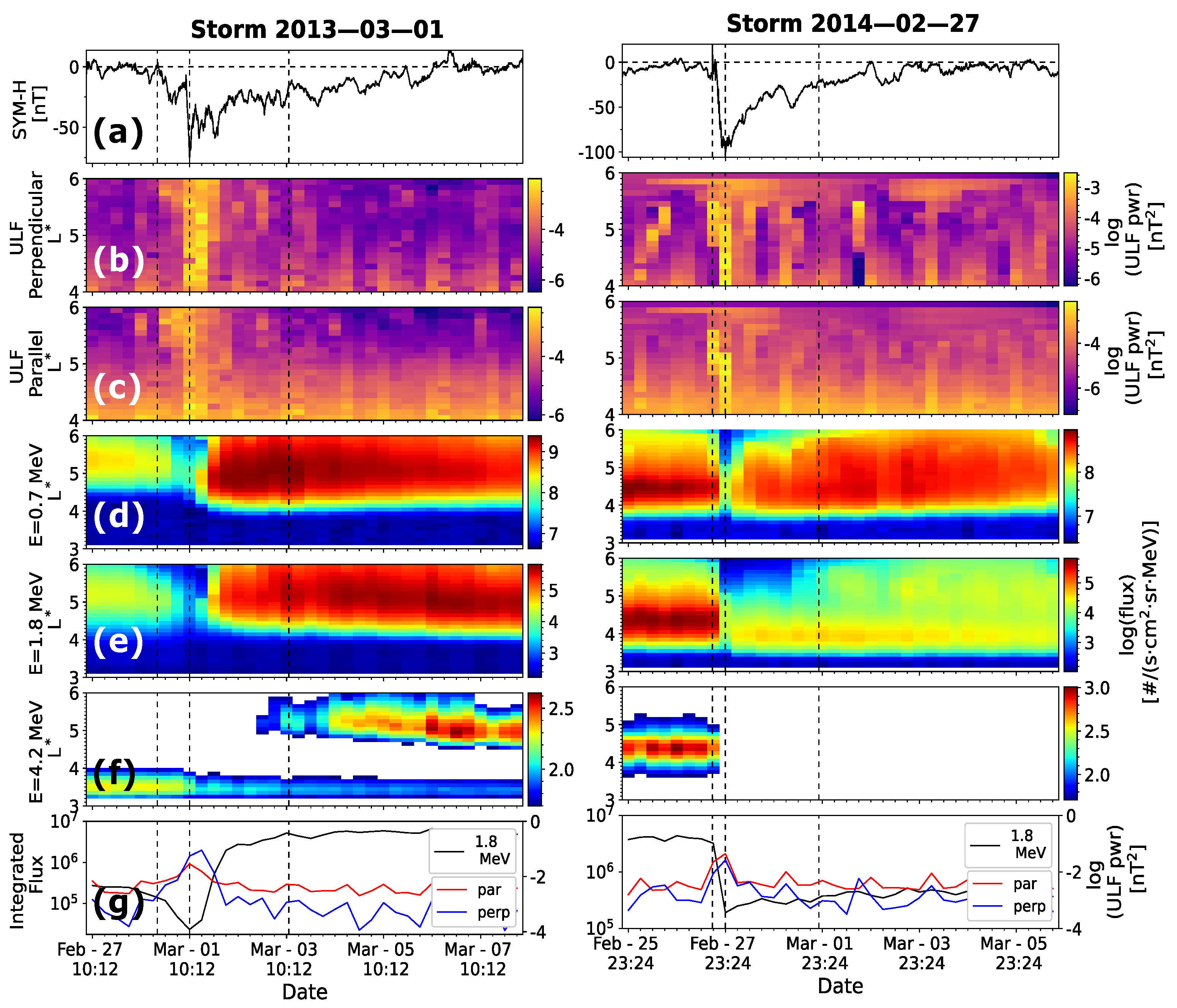
To study the possible correlations between the dynamics of relativistic electrons and ULF wave power during storms, we calculate the ULF power for both parallel and perpendicular fluctuations, integrating the corresponding magnetic power spectral density data within the frequency range from 1 mHz to 10 mHz. Furthermore, we employed the same binning process as used for electron fluxes, involving the spatial and temporal averaging of data with respect to and time. To do so, we considered = 0.1 and Δt = 6 h, averaging the linear ULF power values within each bin. Figure 2 shows an example of the binned ULF power, as well as electron fluxes for two geomagnetic storms that occurred on 1 March 2013 (left) and 27 February 2014 (right). Figure 2a shows the SYM-H index while Figure 2b,c present the ULF power for perpendicular and parallel fluctuations, respectively, binned in time and space. Figure 2d,e,f show the relativistic electron fluxes at energies of 0.7 MeV, 1.8 MeV, and 4.2 MeV, respectively. Figure 2g shows the 1.8 MeV flux integrated over along with the -integrated parallel and perpendicular ULF power. In each event, the following three vertical lines denote key times: the start of the storm (leftmost line), defined by the sudden increase in the SYM-H index if present or by the first noticeable drop; the minimum SYM-H index (central line); and the end of the storm, marked by an 80% recovery in the SYM-H index (rightmost line). The criteria were adopted from Moya et al. [8]. Three time periods are thus established as follows: the main phase, the recovery phase, and the entire duration of the storm. For simplicity, the main phase is defined between the start of the storm and the time of the SYM-H minimum, even though sometimes this includes the sudden storm commencement phase. The recovery phase is defined between the SYM-H minimum and the end of the storm, and the entire storm is between the start and end of the storm. To avoid issues with the binning of the data, main phases shorter than 6 h were not considered. Similarly, if the recovery of the SYM-H index happened faster than in a day, the recovery phase is defined to last 24 h.

Figure 2.
Geomagnetic storms of 1 March 2013 (left) and 27 February 2014 (right). (a) SYM-H index. (b) ULF power for perpendicular fluctuations. (c) ULF power for parallel fluctuations. Both for waves with frequencies between 1 and 10 mHz. (d–f) Electron fluxes of 0.7 MeV, 1.8 MeV, and 4.2 MeV, respectively. Flux values below the background level are shown as white regions. (g) integrated electron flux at 1.8 MeV (black), ULF parallel power (red), and ULF perpendicular power (blue). Black vertical lines represent the start of the storm (left), the SYM-H index minimum (center), and the end of the recovery phase (right).
Figure 2 illustrates the increase and/or decrease of the electron flux, depending on time and for two different storms. The left panel shows an increase in relativistic electron fluxes, mainly for greater than 4.0, across all energy channels during the recovery phase. The flux increase for lower energies is larger, and the response time differs for each and energy. The enhancement is faster for near 5.0 compared to between 4 and 5 in the outer radiation belt. On the other hand, fluxes at less than 4.0 experience a depletion. Similar observations are made for the second storm (right panel). Electron fluxes in the outer radiation belt primarily experience a depletion for all . The SYM-H index, which reflects the intensity of the storm, shows a moderate (left) and a stronger (right) storm, consistent with previous studies showing that the evolution of fluxes depends on electron energy, , or storm intensity [6,8,12,13,21]. Additionally, we observe that the variation in the SYM-H index is similar for different events, with a strong decrease consistent with Lenz’s law during the main phase. Consequently, the terrestrial magnetic field has a recovery time that varies for each storm. Furthermore, the ULF panels of Figure 2b,c show an increase in the occurrence of ULF waves during the storm’s main phase in the 1–10 mHz band. This is corroborated for both storms in Figure 2g. We observe an increase in -integrated ULF power during a geomagnetic storm, while for 1.8 MeV electrons, we note a decrease in the -integrated flux during the storm maximum and then an increase.
After computing and binning the ULF power and electron fluxes, the next step is studying the correlation between the ULF power and the -integrated electron fluxes (adding fluxes over for all the outer radiation belts). The correlations are obtained for each energy channel using all storms considered for this work and separating for the storm period. Specifically, for the analysis, we consider a pre-storm period, which considers 24 h before the storm onset, and a post-storm period, ranging from the end of the recovery phase up to 96 h thereafter. Thus, we calculated the following correlations for both parallel and perpendicular fluctuations with log values: (i) the correlation between the -integrated ULF power over the main phase of the storm, hereafter referred to as “Main phase”, and the ratio of the -integrated electron flux at SYM-H minimum and the maximum -integrated electron flux in the pre-storm period; (ii) the correlation between the -integrated ULF power during the recovery phase, which we will refer to as “Recovery phase”, and the ratio of the maximum -integrated electron flux in the post-storm period and the -integrated electron flux at SYM-H minimum; and (iii) the correlation between the -integrated ULF power over the entire storm, from now on referred to as “Entire Storm”, and the ratio of the maximum -integrated electron flux in the post-storm period and the maximum -integrated electron flux in the pre-storm period. These calculations for -integrated ULF power and -integrated electron fluxes ratios were performed for 101 storms. The correlations are quantified using the Pearson correlation coefficient and the respective p-values for parallel and perpendicular fluctuations in two cases. First, the correlation between ULF power and the differential flux, both integrated across all ; and second, the -integrated ULF power and the differential flux at a given .
It is worth noting that this study primarily focuses on the occurrence of ULF waves. We recognize that numerous other parameters and factors can influence the dynamics of electron fluxes, but they are not included in our current analysis. For example, the behavior of relativistic electrons, especially during storm events, involves loss due to magnetopause shadowing effects; Electromagnetic Ion Cyclotron (EMIC) waves, etc.; and acceleration due to chorus waves. While these factors are important in understanding the complete picture of electron dynamics in the radiation belts, they are beyond the scope of our investigation.
4. Results
Figure 3 shows scatter plots of the previously defined flux ratios and the ULF -integrated power for parallel (red) and perpendicular (blue) fluctuations (top: 4.2 MeV; center: 1.8 MeV; bottom: 0.7 MeV) for the 101 storms considered in this study. With this information, we calculate the Pearson’s correlation coefficients C between the evolution of the relativistic electron fluxes and the -integrated ULF power during storms. The dispersion of the data points in Figure 3, the linear regression fits in each panel, and the correlation coefficients plus the p-values indicate the great variability in the flux responses and ULF power behavior during geomagnetic storms. From Figure 3, we can notice that for at least some energies and some phases, the relation between ULF waves and fluxes could be at least considered to have a linear component, with correlation coefficients getting closer to 0.5. Based on the appreciation that a linear relationship is worth investigating, we will perform a more detailed analysis of the correlation between the two studied quantities.
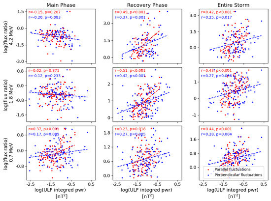
Figure 3.
Ratio of flux evolution and integrated ULF power for each storm phase for the 101 storms in the study. The figure shows the Main Phase (left), the Recovery Phase (center), and the Entire Storm (right). The rows correspond to different electron energies as follows: 4.2 MeV (top), 1.8 MeV (middle), and 0.7 MeV (bottom). The red points correspond to the parallel fluctuations with respect to the background magnetic field, and the blue points correspond to the perpendicular fluctuations. Dashed lines correspond to the linear regression fit for each corresponding dataset.
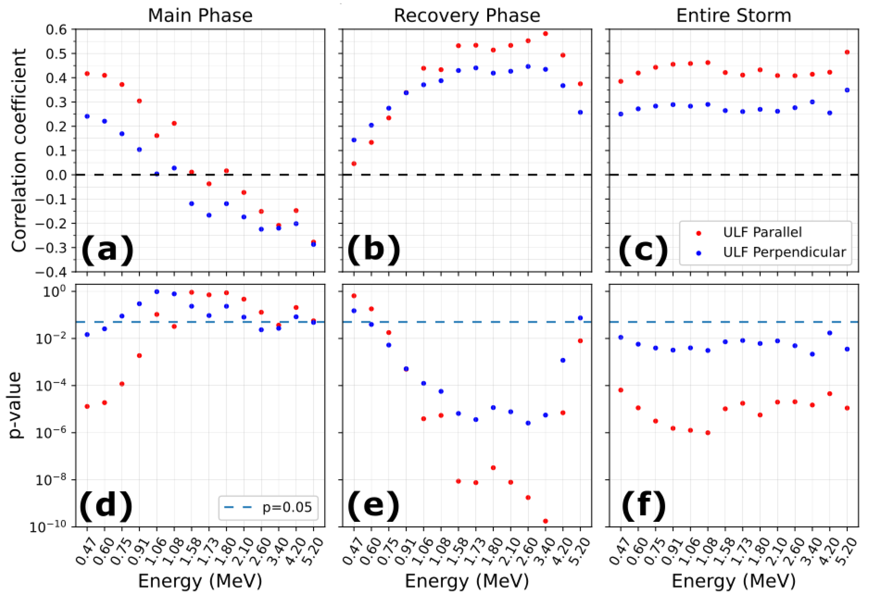
Figure 4 shows, for all available energy channels, the calculated correlation coefficient (top rows), and the statistical significance (bottom rows) assessed through the calculation of the p-value associated with each correlation coefficient. Here we consider as the threshold for good statistical significance within a 95% confidence interval. Figure 4 shows that, in general, the statistical trends followed by the correlation concerning parallel and perpendicular fluctuations are similar, with the difference between them being mostly about the value of the correlation coefficient and the threshold for significance. During the Main Phase of storms (Figure 4a), the correlation coefficient is at a maximum for the lowest energy, and consistently decreases as the energy increases. The peak in correlation is C = 0.42 for 0.47 MeV electrons and parallel fluctuations and C = 0.24 for 0.47 MeV particles and perpendicular fluctuations. Moreover, the p-value shows that the results are statistically significant only for energies <1 MeV and only for parallel fluctuations. During the Recovery Phase (Figure 4b), we observe the opposite behavior than from the Main Phase, this is, the lower energy channels present the lowest correlation coefficients and the lowest statistical significance, but both correlation and significance increase up to the MeV channels, and remains elevated until the 3.4 MeV channel when then they decrease again. We observe higher correlations between parallel ULF wave -integrated power with a peak of C = 0.58 for 3.4 MeV electrons, while for perpendicular fluctuations the peak is C = 0.45 for 2.6 MeV electrons. Finally, Figure 4c shows that for the Entire Storm, the correlations seem to present a somewhat additive behavior, and thus, the correlation remains relatively constant and moderately high for all energy channels, while the statistical significance is always high. In this case, the maximum correlation for parallel fluctuations is 0.51 for 5.2 MeV, while for perpendicular fluctuations is 0.35 in 5.20 MeV.

Figure 4.
Correlation coefficient (top panels) and p-values (bottom panels) obtained for the comparison between integrated ULF power and flux evolution ratio for all considered geomagnetic storms. Columns correspond to storm phases: Main Phase (a,d), Recovery Phase (b,e), and Entire Storm (c,f). Red and blue dots indicate parallel and perpendicular fluctuations, respectively. The light blue line in the bottom panels indicates the 5% p-value threshold ().
To further quantify the correlation between ULF power and changes in the radiation belt during geomagnetic storms, we repeated the calculation but computed the correlation coefficient considering individual values (within bins with ) for the ratio of electron fluxes, and the ULF power integrated between . To explore the possibility that linear regression does not fully capture the connection between the data, we also calculated a normalized mutual information score. The mutual information coefficient is calculated as
with corresponding to the joint probability mass function between X and Y and and the marginal probability mass functions of X and Y, respectively. The mutual information score indicates the mutual dependence of the two variables and can capture non-linear dependence between them. It is a technique that has been used successfully in many problems in magnetospheric physics [66,67,68,69,70]. However, as the mutual information score is not bounded to a maximum value, it can be hard to interpret. To improve our explainability, we have calculated the normalized mutual information score in the following way
where can be interpreted as the entropy of X. Figure 5 and Figure 6 present the correlation coefficients (left) and normalized mutual information scores (right) for all energy channels and fluctuations parallel and perpendicular to the background field, respectively. From top to bottom, the figures show the calculated values for the Main Phase (top), Recovery Phase (center), and Entire Storm (bottom). The contours show the region in which the p-value is equal to the 5% we are considering as statistically significant. The regions with p-value and p-value are indicated as they are going to be used to guide the discussion. It is important to note that the contours of the p-value were also drawn on top of the right side, showing the normalized mutual information scores as a visual guide, but a second statistical test was not performed. It can be appreciated that both Figure 5 and Figure 6 are generally consistent with the findings of Figure 4, but at the same time, the by calculation shows a very complex scenario at different energies and locations.
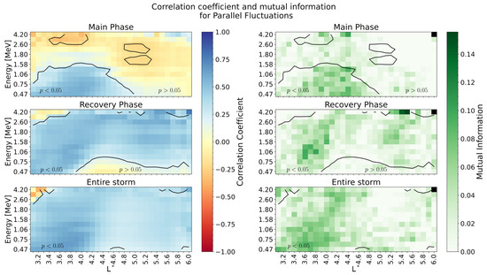
Figure 5.
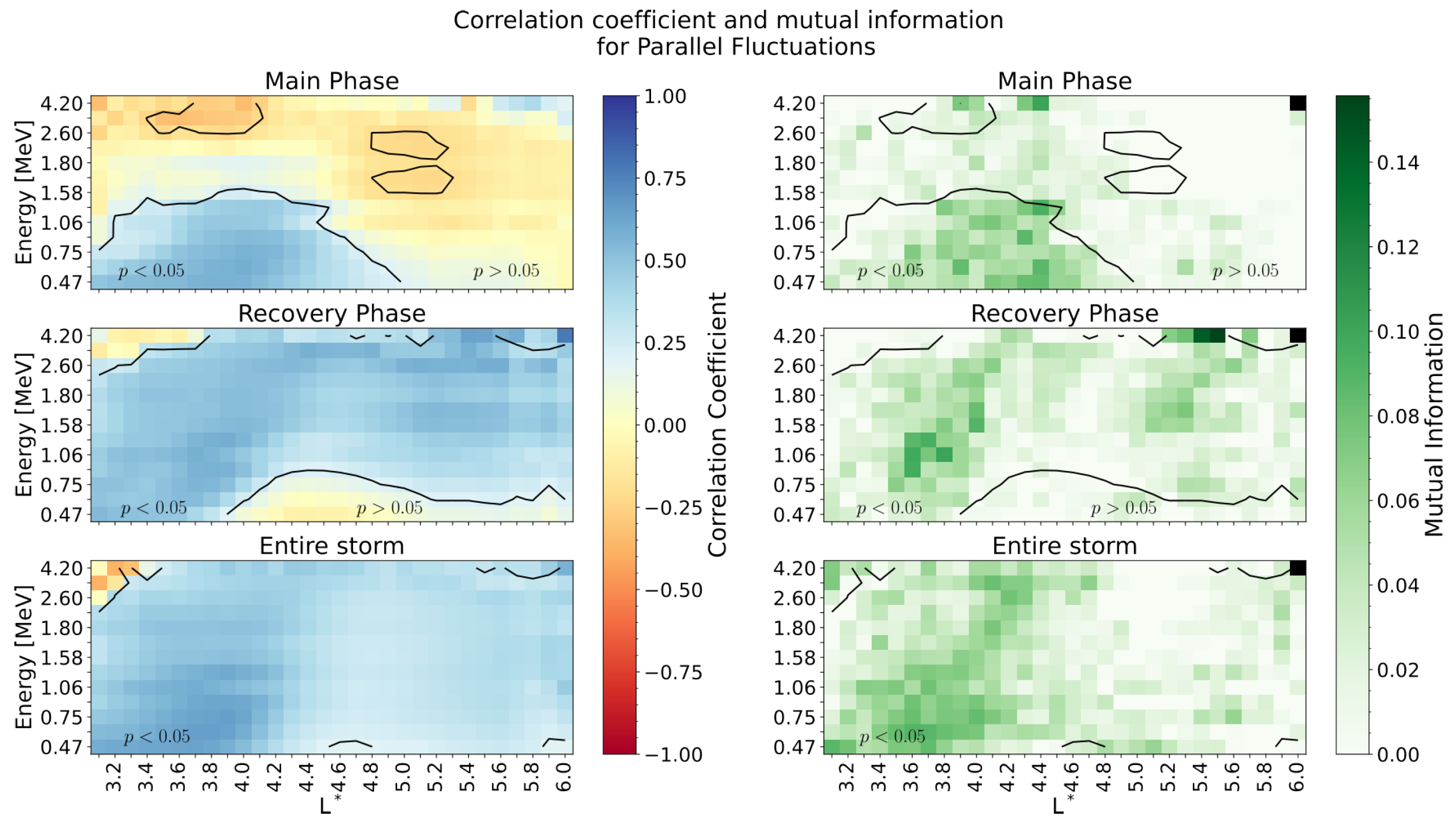
Correlation coefficient (left) and normalized mutual information score (right) for the comparison between integrated ULF power for parallel fluctuations and the L-dependent flux evolution ratio, for all considered geomagnetic storms. Panels show the Main Phase (top), the Recovery Phase (center), and the Entire Storm (bottom). The contours indicate the regions in which the p-value .

Figure 6.
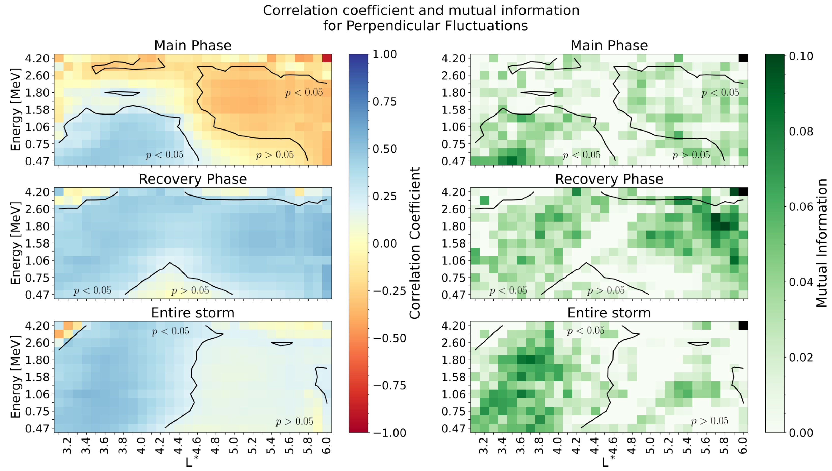
Correlation coefficient (left) and normalized mutual information score (right) for comparison between ULF power for perpendicular fluctuations and the flux evolution ratio, for all considered geomagnetic storms. Panels show the Main Phase (top), the Recovery Phase (center), and the Entire Storm (bottom). The contours indicate the regions in which the p-value .
The top panels in Figure 5 confirm that the lower energies are the most correlated with the integrated wave power during the Main Phase. However, the correlation is significantly higher for and from energies up to 1.6 MeV at . For there is a statistically significant anticorrelation for energies between and MeV. In the Recovery Phase (middle panels), we observe positive correlations throughout the entire region for most energy channels. Remarkably, there is a very high statistical significance for most of the regions in which the fluxes are highly correlated. The maximum correlation coefficient values are around at for MeV. Additionally, we observe C values around for for energies lower than ∼ 1 MeV. It is also clear that the correlations for the lower energies at the heart of the belt and at the highest energies, particularly around the borders of the system are very low, or slightly negative, but with poor statistical significance. When considering the Entire Storm (bottom panels), the “additive” effect mentioned earlier seems to be in effect again, and the majority of the obtained results are highly significant with a relatively high correlation. The maximum significant correlation coefficient is for MeV at . For , we obtain , particularly for energies larger than 2.6 MeV. The normalized mutual information (NMI) scores are consistent in showing that the regions with the highest correlations correspond to the regions with the highest NMI scores. For example, for the Main Phase, the NMI indicates that the region of positive correlation, lower energy channels, and are the ones that contain the most information. Similar results are seen for the Recovery Phase and Entire Storm. It is interesting also that both the correlation and NMI scores are relatively low in the regions we are considering as “statistically relevant”. This could be interpreted as an indication that a connection between ULF Power and fluxes exists but is subtle and cannot be easily identified as linear or non-linear.
In the case of perpendicular fluctuations, at first sight, Figure 6 follows the same structure as Figure 5 but with some key differences worth noting. During the Main Phase (top row), we observe a similar region of high correlation at low and low energy channels with a peak of at for 0.47 MeV. However, there is a very strong anticorrelation for most energy channels as increases (peak at in MeV). It is not unreasonable to think that this opposite behavior at smaller or larger values is, in part, affecting the results in Figure 4, where fluxes are less correlated with perpendicular fluctuations than with parallel fluctuations. During the Recovery Phase (middle row), the results are in agreement with Figure 5, indicating that both parallel and perpendicular ULF power correlate similarly with the electron fluxes across the same energies and . For perpendicular fluctuations, we found the highest values of at 6.0 and slightly lower for most of the energy channels. Finally, when considering the Entire Storm event (bottom row), again we observe that the effects from the Main Phase and Recovery Phase tend to add to each other, in this case resulting in a highly correlated region for , with a peak of for energies lower than 1.8 MeV. The normalized mutual information (NMI) scores in this case again seem to highlight the statistically significant regions of the plot with the highest correlations as the ones containing more mutual information. Perhaps the most striking difference between Figure 5 and Figure 6 is that the perpendicular fluctuations show a stronger NMI score in the energies MeV and the region , which is not as clearly captured by the correlation coefficient. It is perhaps in this region where we could maybe consider that some non-linear connection exists between ULF waves and fluxes that could be further explored in the future. This is despite the NMI being relatively low and comparable to the scores shown for parallel fluctuations.
5. Discussion and Conclusions
We have performed a statistical study of the correlation between the integrated ULF power between 1 mHz and 10 mHz and the evolution of the relativistic electron fluxes in the outer radiation belt during different phases of a geomagnetic storm, determined by the ratio of the fluxes at different stages of each storm. The three different time intervals analyzed were the main phase of the storm, where we calculated the ratio between the fluxes at the time when SYM-H minimum occurred and the maximum fluxes pre-storm; the recovery phase of the storm, where we calculated the ratio between the maximum fluxes at the end of the recovery phase and the fluxes at the time of SYM-H minimum; and the entire storm, with the ratio considering the maximum fluxes at the end of the recovery phase versus the maximum fluxes pre-storm. Our data set contained 101 storms between 1 January 2013 and 30 November 2018. We separated the waves between fluctuations parallel and perpendicular to the background magnetic field to study differences in the correlations associated with the different oscillation modes. By using the Van Allen Probes ECT data, particularly the MagEIS and REPT instruments, we were able to study the energy range between 470 keV and 5.2 MeV.
It is important to note that in this work, we considered all storms, regardless of whether they resulted in a general increase or decrease in electron fluxes for different phases, and therefore, it is expected that the correlation coefficients are somewhat reduced by the multitude of processes occurring during each storm event. This is further reinforced by the normalized mutual information score, which tends to indicate some connection between the studied quantities that is likely real but subtle. Moreover, we include all storms, regardless of whether there was a preconditioning of the belt with abnormally elevated or reduced fluxes. Still, Figure 3 and Figure 4 show that a correlation exists between the integrated ULF power and the dynamics of the outer radiation belt for most studied energy channels. In particular, Figure 4 shows that when considering the entire duration of the storms, there is a high correlation in most energy channels for parallel fluctuations and a slightly lower correlation, that is also relatively similar across channels, for perpendicular fluctuations. Interestingly, the relatively constant correlation coefficient across energy channels seems to be the result of some additive influence from the evolution of the outer belt during the Main Phase and the Recovery Phase. During the Main Phase of the storm, the correlation is the highest for the lowest energy channel, and it decreases as energy increases with a shift to anticorrelation for MeV. The correlation at low energies could be associated with a strong inward radial diffusion during storm main phase, while the anticorrelation at high energies could be associated with outward radial diffusion and losses to the magnetopause [71,72]. The caveat in our results is that the anticorrelation for higher energy channels is of low statistical significance. In contrast, during the Recovery Phase, the correlation coefficient increases as the energy increases, and for energies above 0.75 MeV, it is statistically sound. A possible explanation for this behavior during the different phases of the storm is the fact that lower energy channels can respond faster to abrupt changes, such as those seen during the Main Phase, while during the Recovery Phase, the ongoing energization processes tend to affect more consistently the higher energies, in which case, a correlation with ULF activity is likely to be important, as we know that ULF activity can lead to energization. It is important to mention that the results are also consistent with the two-step acceleration process of radiation belt electrons [29,73,74]. In Figure 4, for all the correlations that can be considered significant (i.e., the -value is lower than ), it is consistently found that the ULF power associated with parallel oscillations correlates better with the rate of flux changes than the ULF power associated with perpendicular oscillations. As parallel fluctuations correspond to the compressional component of ULF waves [50], these results are in agreement with previously reported drift resonance wave–particle interactions between radiation belt electrons and compressional toroidal waves [42].
Figure 5 and Figure 6 present an expanded view of the same correlation analysis. Here, we compared the integrated ULF wave power calculated for all outer radiation belts with the rate of change of the electrons at each , with and for . Figure 5 presents the correlation coefficients and NMI score for variations parallel to the background field and Figure 6 for variations perpendicular to the background field. When observing the results of the Main Phase, there is some similarity in the way the different wave modes affect the inner region of the belt at low energies, which corresponds to the region with the highest correlation, but there is also a striking difference in the external region of the belt at higher energies MeV, where the perpendicular fluctuations show a stronger anti-correlation. This behavior could be attributed to quick energization processes and the overpopulation of particles resulting from mechanisms such as radial transport at low energies and the efficient removal processes that affect the outer belt during the main phase of a storm. The results are consistent with the enhancement for radial diffusion in the perpendicular case [40,43,47]. In the regions with low statistical significance, the fast response to the geomagnetic storm and other factors might be influencing the lack of significant correlations. In the case of perpendicular fluctuations, it is plausible that they could contribute to a decrease in the electron flux, which could further impact the observed correlations. Furthermore, if we examine the results reported by Pinto et al. [17], electrons at larger L values may experience a depletion in flux during the main phase of a geomagnetic storm.
The results of the Recovery Phase for Figure 5 and Figure 6 are relatively similar, but with higher correlations found for parallel fluctuations. This suggests that fluctuations generated by ULF waves could play an essential role in the increase of electron fluxes during the recovery phase of a geomagnetic storm, except for lower energies (0.47–0.75 MeV) or at very high energies. The perpendicular fluctuations show one of the highest NMI scores in the region and energies MeV, which could be indicative of some non-linear behavior being more important than the linear correlation shows. The resonance between the ULF waves and particles could be one of the reasons for these observed results. These findings suggest that the resonance between ULF waves and electrons could be an important physical process in driving changes in the flux of the radiation belt during a geomagnetic storm. It is likely that this mechanism violates the third adiabatic invariant and subsequently drives radial diffusion [75]. That being said, it is imperative to emphasize that our study is focused on global-scale interactions, taking into account the substantial time of wave propagation required to effectively resonate with particles in the region. As mentioned earlier, the Entire Storm analysis behaves as if the Main Phase and Recovery Phase were added, and as such, presents stronger correlations. An unusual result is obtained for perpendicular fluctuations, where the strong anticorrelation for during the Main Phase and a strong correlation in the same region during the Recovery Phase cancel out during the Entire Storm, resulting in most of the region not correlating at all between fluxes and ULF integrated perpendicular power.
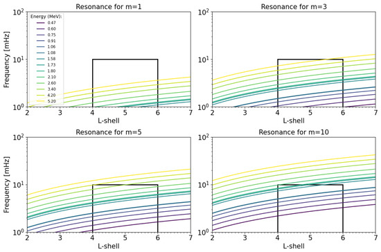
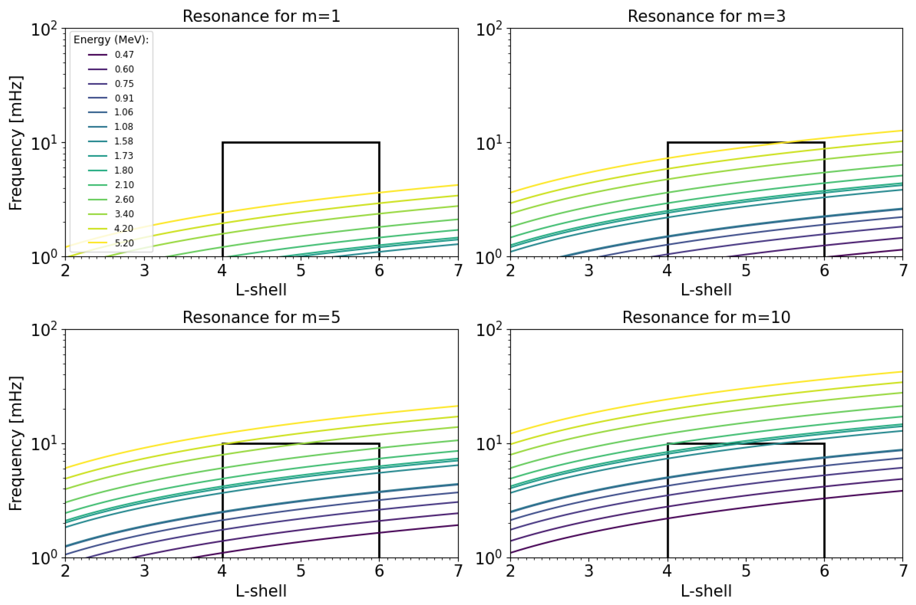
To assess the possibility that significant correlations indicate resonant interactions, Figure 7 evaluates Equation (1) for (drift resonance) and small values of the azimuthal wavenumber ( 1, 3, 5, and 10), expected for toroidal ULF waves [76]. Colored lines correspond to resonant frequencies as a function of for different energies. Each panel includes a black square indicating resonances within our interest zone of drift resonance between ULF waves, with frequencies between 1 and 10 mHz, and relativistic electrons in the outer radiation belt at . Results show that, in general, higher energy particles can resonate with higher frequency waves. Inside the interest zone, multi-MeV electrons may resonate with less than 10 mHz ULF waves only for (top left panel in the figure). On the contrary, hundreds of keV electrons may undergo drift resonance only for a larger m value (bottom right panel). In addition, ∼1 MeV electrons may resonate with ULF waves for intermediate values of the azimuthal wavenumber ( 3, 5). In summary, for all considered energies, our results indicate that the drift resonance with less than 10 mHz ULF waves may occur in the interest zone.
As our study was of broad scope, considering every geomagnetic storm despite its electron flux outcome, further analysis and investigation are necessary to deepen our understanding of the specific mechanisms and processes involved in the resonance between ULF waves and electrons and how they contribute to the changes observed in the radiation belt during geomagnetic storms. For example, including the experimental m-value could be helpful to find out what type of waves are interacting with the electrons and to detail the resonant interaction in each geomagnetic storm in the analysis. Additionally, it seems reasonable to think that, particularly in narrow bands, a study of the evolution of the phase space density of the electrons could yield better results in determining the effect ULF waves may have on the electron populations. Overall, our findings highlight the complex nature of the relationship between ULF waves and electron flux behavior within the radiation belt. Further studies considering more parameters could clarify these results, improve the possible correlation between physical processes and the dynamics of the radiation belts during storms, and even prove a causal relationship. We expect to further explore these ideas, broaden the frequency spectrum, study the types of precursors, and correlate with the evolution of the SYM-H index, AE, among others.
Supplementary Materials
The following supporting information can be downloaded at: https://www.mdpi.com/article/10.3390/universe11050151/s1, Table S1: List of geomagnetic storms between 17 January 2013 and 5 November 2018 including their minimum SYM-H index; Figure S2: The number of data points that typically go into each bin for the electron fluxes.
Author Contributions
Conceptualization, P.S.M., C.L. and V.A.P.; methodology, P.S.M., C.L. and V.A.P.; software, C.L. and J.S.; validation, P.S.M., V.A.P., C.L. and B.Z.-Q.; resources, P.S.M., V.A.P.; writing—original draft preparation, C.L., V.A.P. and P.S.M.; writing—review and editing, P.S.M., V.A.P., B.Z.-Q. and J.S.; visualization, C.L. and J.S.; supervision, P.S.M. and V.A.P. All authors have read and agreed to the published version of the manuscript.
Funding
This research was funded by ANID, Chile, through National Graduate Scholarship No. 50220081 (C.L.), FONDECYT grants No. 1211144 (C.L., P.S.M.), No. 1240281 (P.S.M., V.A.P.), No. 11251905 (V.A.P.), No. 3250884 (B.Z.-Q.); and SIA Grant SA77210112 (V.A.P.). We also thank DICYT Project 042331PA_Ayudante (V.A.P., J.S.), DICYT Project 042131PA_JUVI (V.A.P., B.Z.-Q.), and DICYT Regular Project 042431PA (V.A.P.).
Data Availability Statement
The Van Allen Probes ECT-REPT, ECT-MagEIS, and EMFISIS data are available from http://cdaweb.gsfc.nasa.gov (accessed on 30 April 2025). SYM-H data are available from http://omniweb.gsfc.nasa.gov (accessed on 30 April 2025). The complete list of geomagnetic storms and their respective minimum SYM-H values can be found in the Supporting Information.
Acknowledgments
We acknowledge the use of the Van Allen Probes mission through NASA/GSFC’s Space Physics Data Facility’s OMNIWeb and CDAWeb services, and OMNI data.
Conflicts of Interest
The authors declare no conflicts of interest.
References
- Baker, D.N. The Occurrence of Operational Anomalies in Spacecraft and Their Relationship to Space Weather. IEEE Trans. Plasma Sci. 2000, 28, 2007–2016. [Google Scholar] [CrossRef]
- Wrenn, G.L.; Rodgers, D.J.; Ryden, K.A. A Solar Cycle of Spacecraft Anomalies Due to Internal Charging. Ann. Geophys. 2002, 20, 953–956. [Google Scholar] [CrossRef]
- Wrenn, G. Chronology of ‘Killer’ Electrons: Solar Cycles 22 and 23. J. Atmos. Sol.-Terr. Phys. 2009, 71, 1210–1218. [Google Scholar] [CrossRef]
- Horne, R.B.; Glauert, S.A.; Meredith, N.P.; Boscher, D.; Maget, V.; Heynderickx, D.; Pitchford, D. Space Weather Impacts on Satellites and Forecasting the Earth’s Electron Radiation Belts with SPACECAST. Space Weather 2013, 11, 169–186. [Google Scholar] [CrossRef]
- Hands, A.D.P.; Ryden, K.A.; Meredith, N.P.; Glauert, S.A.; Horne, R.B. Radiation Effects on Satellites During Extreme Space Weather Events. Space Weather 2018, 16, 1216–1226. [Google Scholar] [CrossRef]
- Reeves, G.D.; McAdams, K.L.; Friedel, R.H.W.; O’Brien, T.P. Acceleration and Loss of Relativistic Electrons during Geomagnetic Storms. Geophys. Res. Lett. 2003, 30, 1529. [Google Scholar] [CrossRef]
- Turner, D.L.; O’Brien, T.P.; Fennell, J.F.; Claudepierre, S.G.; Blake, J.B.; Kilpua, E.K.J.; Hietala, H. The Effects of Geomagnetic Storms on Electrons in Earth’s Radiation Belts. Geophys. Res. Lett. 2015, 42, 9176–9184. [Google Scholar] [CrossRef]
- Moya, P.S.; Pinto, V.A.; Sibeck, D.G.; Kanekal, S.G.; Baker, D.N. On the Effect of Geomagnetic Storms on Relativistic Electrons in the Outer Radiation Belt: Van Allen Probes Observations. J. Geophys. Res. Space Phys. 2017, 122, 11100–11108. [Google Scholar] [CrossRef]
- Turner, D.L.; Kilpua, E.K.J.; Hietala, H.; Claudepierre, S.G.; O’Brien, T.P.; Fennell, J.F.; Blake, J.B.; Jaynes, A.N.; Kanekal, S.; Baker, D.N.; et al. The Response of Earth’s Electron Radiation Belts to Geomagnetic Storms: Statistics from the Van Allen Probes Era Including Effects From Different Storm Drivers. J. Geophys. Res. Space Phys. 2019, 124, 1013–1034. [Google Scholar] [CrossRef]
- Miyoshi, Y.; Kataoka, R. Flux Enhancement of the Outer Radiation Belt Electrons after the Arrival of Stream Interaction Regions. J. Geophys. Res. Space Phys. 2008, 113, A03S09. [Google Scholar] [CrossRef]
- Pandya, M.; Bhaskara, V.; Ebihara, Y.; Kanekal, S.G.; Baker, D.N. Variation of Radiation Belt Electron Flux During CME- and CIR-Driven Geomagnetic Storms: Van Allen Probes Observations. J. Geophys. Res. Space Phys. 2019, 124, 6524–6540. [Google Scholar] [CrossRef]
- Zhao, H.; Li, X. Inward Shift of Outer Radiation Belt Electrons as a Function of Dst Index and the Influence of the Solar Wind on Electron Injections into the Slot Region. J. Geophys. Res. Space Phys. 2013, 118, 756–764. [Google Scholar] [CrossRef]
- Pinto, V.A.; Bortnik, J.; Moya, P.S.; Lyons, L.R.; Sibeck, D.G.; Kanekal, S.G.; Spence, H.E.; Baker, D.N. Radial Response of Outer Radiation Belt Relativistic Electrons During Enhancement Events at Geostationary Orbit. J. Geophys. Res. Space Phys. 2020, 125, e2019JA027660. [Google Scholar] [CrossRef]
- Lyons, L.R.; Lee, D.Y.; Thorne, R.M.; Horne, R.B.; Smith, A.J. Solar Wind-Magnetosphere Coupling Leading to Relativistic Electron Energization during High-Speed Streams. J. Geophys. Res. 2005, 110, A11202. [Google Scholar] [CrossRef]
- Lyons, L.; Lee, D.Y.; Kim, H.J.; Hwang, J.; Thorne, R.; Horne, R.; Smith, A. Solar-Wind–Magnetosphere Coupling, Including Relativistic Electron Energization, during High-Speed Streams. J. Atmos. -Sol.-Terr. Phys. 2009, 71, 1059–1072. [Google Scholar] [CrossRef]
- Kim, H.J.; Lyons, L.; Pinto, V.; Wang, C.P.; Kim, K.C. Revisit of Relationship between Geosynchronous Relativistic Electron Enhancements and Magnetic Storms. Geophys. Res. Lett. 2015, 42, 6155–6161. [Google Scholar] [CrossRef]
- Pinto, V.A.; Bortnik, J.; Moya, P.S.; Lyons, L.R.; Sibeck, D.G.; Kanekal, S.G.; Spence, H.E.; Baker, D.N. Characteristics, Occurrence, and Decay Rates of Remnant Belts Associated with Three-Belt Events in the Earth’s Radiation Belts. Geophys. Res. Lett. 2018, 45, 12099–12107. [Google Scholar] [CrossRef]
- Mann, I.; O’Brien, T.; Milling, D. Correlations between ULF Wave Power, Solar Wind Speed, and Relativistic Electron Flux in the Magnetosphere: Solar Cycle Dependence. J. Atmos. -Sol.-Terr. Phys. 2004, 66, 187–198. [Google Scholar] [CrossRef]
- Georgiou, M.; Daglis, I.A.; Rae, I.J.; Zesta, E.; Sibeck, D.G.; Mann, I.R.; Balasis, G.; Tsinganos, K. Ultralow Frequency Waves as an Intermediary for Solar Wind Energy Input Into the Radiation Belts. J. Geophys. Res. Space Phys. 2018, 123, 10090–10108. [Google Scholar] [CrossRef]
- Stepanova, M.; Pinto, V.; Antonova, E. Regarding the Relativistic Electron Dynamics in the Outer Radiation Belt: A Historical View. Rev. Mod. Plasma Phys. 2024, 8, 25. [Google Scholar] [CrossRef]
- Turner, D.L.; Angelopoulos, V.; Li, W.; Hartinger, M.D.; Usanova, M.; Mann, I.R.; Bortnik, J.; Shprits, Y. On the Storm-Time Evolution of Relativistic Electron Phase Space Density in Earth’s Outer Radiation Belt. J. Geophys. Res. Space Phys. 2013, 118, 2196–2212. [Google Scholar] [CrossRef]
- Boyd, A.J.; Spence, H.E.; Huang, C.L.; Reeves, G.D.; Baker, D.N.; Turner, D.L.; Claudepierre, S.G.; Fennell, J.F.; Blake, J.B.; Shprits, Y.Y. Statistical Properties of the Radiation Belt Seed Population. J. Geophys. Res. Space Phys. 2016, 121, 7636–7646. [Google Scholar] [CrossRef]
- Antonova, E.E.; Stepanova, M.V.; Moya, P.S.; Pinto, V.A.; Vovchenko, V.V.; Ovchinnikov, I.L.; Sotnikov, N.V. Processes in Auroral Oval and Outer Electron Radiation Belt. Earth Planets Space 2018, 70, 127. [Google Scholar] [CrossRef]
- Katsavrias, C.; Daglis, I.A.; Li, W. On the Statistics of Acceleration and Loss of Relativistic Electrons in the Outer Radiation Belt: A Superposed Epoch Analysis. J. Geophys. Res. Space Phys. 2019, 124, 2755–2768. [Google Scholar] [CrossRef]
- Lejosne, S.; Allison, H.J.; Blum, L.W.; Drozdov, A.Y.; Hartinger, M.D.; Hudson, M.K.; Jaynes, A.N.; Ozeke, L.; Roussos, E.; Zhao, H. Differentiating Between the Leading Processes for Electron Radiation Belt Acceleration. Front. Astron. Space Sci. 2022, 9, 896245. [Google Scholar] [CrossRef]
- Wing, S.; Johnson, J.R.; Turner, D.L.; Ukhorskiy, A.Y.; Boyd, A.J. Untangling the Solar Wind and Magnetospheric Drivers of the Radiation Belt Electrons. J. Geophys. Res. Space Phys. 2022, 127, e2021JA030246. [Google Scholar] [CrossRef]
- Osmane, A.; Kilpua, E.; George, H.; Allanson, O.; Kalliokoski, M. Radial Transport in the Earth’s Radiation Belts: Linear, Quasi-linear, and Higher-order Processes. Astrophys. J. Suppl. Ser. 2023, 269, 44. [Google Scholar] [CrossRef]
- Manshour, P.; Papadimitriou, C.; Balasis, G.; Paluš, M. Causal Inference in the Outer Radiation Belt: Evidence for Local Acceleration. Geophys. Res. Lett. 2024, 51, e2023GL107166. [Google Scholar] [CrossRef]
- Jaynes, A.N.; Baker, D.N.; Singer, H.J.; Rodriguez, J.V.; Loto’aniu, T.M.; Ali, A.F.; Elkington, S.R.; Li, X.; Kanekal, S.G.; Claudepierre, S.G.; et al. Source and Seed Populations for Relativistic Electrons: Their Roles in Radiation Belt Changes. J. Geophys. Res. Space Phys. 2015, 120, 7240–7254. [Google Scholar] [CrossRef]
- Millan, R.M.; Baker, D.N. Acceleration of Particles to High Energies in Earth’s Radiation Belts. Space Sci. Rev. 2012, 173, 103–131. [Google Scholar] [CrossRef]
- Zong, Q. Magnetospheric Response to Solar Wind Forcing: Ultra-Low-Frequency Wave–Particle Interaction Perspective. Ann. Geophys. 2022, 40, 121–150. [Google Scholar] [CrossRef]
- Simms, L.E.; Engebretson, M.J.; Rodger, C.J.; Dimitrakoudis, S.; Mann, I.R.; Chi, P.J. The Combined Influence of Lower Band Chorus and ULF Waves on Radiation Belt Electron Fluxes at Individual L -Shells. J. Geophys. Res. Space Phys. 2021, 126, e2020JA028755. [Google Scholar] [CrossRef]
- Elkington, S.R.; Hudson, M.K.; Chan, A.A. Acceleration of Relativistic Electrons via Drift-resonant Interaction with Toroidal-mode Pc-5 ULF Oscillations. Geophys. Res. Lett. 1999, 26, 3273–3276. [Google Scholar] [CrossRef]
- Mager, P.N.; Klimushkin, D.Y. Spatial Localization and Azimuthal Wave Numbers of Alfvén Waves Generated by Drift-Bounce Resonance in the Magnetosphere. Ann. Geophys. 2005, 23, 3775–3784. [Google Scholar] [CrossRef]
- O’Brien, T.P.; McPherron, R.L.; Sornette, D.; Reeves, G.D.; Friedel, R.; Singer, H.J. Which Magnetic Storms Produce Relativistic Electrons at Geosynchronous Orbit? J. Geophys. Res. Space Phys. 2001, 106, 15533–15544. [Google Scholar] [CrossRef]
- Chen, L.; Hasegawa, A. A theory of long-period magnetic pulsations: 1. Steady state excitation of field line resonance. J. Geophys. Res. 1974, 79, 1024–1032. [Google Scholar] [CrossRef]
- Southwood, D.J.; Kivelson, M.G. The magnetohydrodynamic response of the magnetospheric cavity to changes in solar wind pressure. J. Geophys. Res. Space Phys. 1990, 95, 2301–2309. [Google Scholar] [CrossRef]
- Di Matteo, S.; Villante, U.; Viall, N.; Kepko, L.; Wallace, S. On Differentiating Multiple Types of ULF Magnetospheric Waves in Response to Solar Wind Periodic Density Structures. J. Geophys. Res. Space Phys. 2022, 127, e2021JA030144. [Google Scholar] [CrossRef]
- Marchezi, J.P.; Dai, L.; Alves, L.R.; Da Silva, L.A.; Sibeck, D.G.; Lago, A.D.; Souza, V.M.; Jauer, P.R.; Veira, L.E.A.; Cardoso, F.R.; et al. Electron Flux Variability and Ultra-Low Frequency Wave Activity in the Outer Radiation Belt Under the Influence of Interplanetary Coronal Mass Ejections and High-Speed Solar Wind Streams: A Statistical Analysis From the Van Allen Probes Era. J. Geophys. Res. Space Phys. 2022, 127, e2021JA029887. [Google Scholar] [CrossRef]
- Elkington, S.R.; Hudson, M.K.; Chan, A.A. Resonant Acceleration and Diffusion of Outer Zone Electrons in an Asymmetric Geomagnetic Field. J. Geophys. Res. Space Phys. 2003, 108, 2001JA009202. [Google Scholar] [CrossRef]
- Elkington, S.R.; Chan, A.A.; Wiltberger, M. Global Structure of ULF Waves During the 24–26 September 1998 Geomagnetic Storm. In Geophysical Monograph Series; Summers, D., Mann, I.R., Baker, D.N., Schulz, M., Eds.; American Geophysical Union: Washington, DC, USA, 2013; pp. 127–138. [Google Scholar] [CrossRef]
- Li, L.; Zhou, X.Z.; Omura, Y.; Zong, Q.G.; Rankin, R.; Chen, X.R.; Liu, Y.; Yue, C.; Fu, S.Y. Drift Resonance Between Particles and Compressional Toroidal ULF Waves in Dipole Magnetic Field. J. Geophys. Res. Space Phys. 2021, 126, e2020JA028842. [Google Scholar] [CrossRef]
- Ukhorskiy, A.Y.; Takahashi, K.; Anderson, B.J.; Korth, H. Impact of Toroidal ULF Waves on the Outer Radiation Belt Electrons. J. Geophys. Res. Space Phys. 2005, 110, 2005JA011017. [Google Scholar] [CrossRef]
- Zong, Q.G.; Zhou, X.Z.; Wang, Y.F.; Li, X.; Song, P.; Baker, D.N.; Fritz, T.A.; Daly, P.W.; Dunlop, M.; Pedersen, A. Energetic Electron Response to ULF Waves Induced by Interplanetary Shocks in the Outer Radiation Belt. J. Geophys. Res. Space Phys. 2009, 126, e2020JA028842. [Google Scholar] [CrossRef]
- Su, Z.; Zhu, H.; Xiao, F.; Zong, Q.G.; Zhou, X.Z.; Zheng, H.; Wang, Y.; Wang, S.; Hao, Y.X.; Gao, Z.; et al. Ultra-Low-Frequency Wave-Driven Diffusion of Radiation Belt Relativistic Electrons. Nat. Commun. 2015, 6, 10096. [Google Scholar] [CrossRef]
- Drozdov, A.Y.; Blum, L.W.; Hartinger, M.; Zhao, H.; Lejosne, S.; Hudson, M.K.; Allison, H.J.; Ozeke, L.; Jaynes, A. Radial Transport vs. Local Acceleration: The Long-standing Debate. Earth Space Sci. 2022, 9, e2022EA002216. [Google Scholar] [CrossRef]
- Murphy, K.R.; Inglis, A.R.; Sibeck, D.G.; Rae, I.J.; Watt, C.E.J.; Silveira, M.; Plaschke, F.; Claudepierre, S.G.; Nakamura, R. Determining the Mode, Frequency, and Azimuthal Wave Number of ULF Waves During a HSS and Moderate Geomagnetic Storm. J. Geophys. Res. Space Phys. 2018, 123, 6457–6477. [Google Scholar] [CrossRef]
- Stix, T.H. Waves in Plasmas; American Institute of Physics: New York, NY, USA, 1992. [Google Scholar]
- Takahashi, K.; Crabtree, C.; Ukhorskiy, A.Y.; Boyd, A.; Denton, R.E.; Turner, D.; Gkioulidou, M.; Vellante, M.; Spence, H.E. Van Allen Probes Observations of Symmetric Stormtime Compressional ULF Waves. J. Geophys. Res. Space Phys. 2022, 127, e2021JA030115. [Google Scholar] [CrossRef]
- Kivelson, M.G. ULF Waves from the Ionosphere to the Outer Planets. In Geophysical Monograph Series; Takahashi, K., Chi, P.J., Denton, R.E., Lysak, R.L., Eds.; American Geophysical Union: Washington, DC, USA, 2006; Volume 169, pp. 11–30. [Google Scholar] [CrossRef]
- Zong, Q.; Wang, Y.; Yuan, C.; Yang, B.; Wang, C.; Zhang, X. Fast Acceleration of “Killer” Electrons and Energetic Ions by Interplanetary Shock Stimulated ULF Waves in the Inner Magnetosphere. Chin. Sci. Bull. 2011, 56, 1188–1201. [Google Scholar] [CrossRef]
- Rae, I.J.; Murphy, K.R.; Watt, C.E.J.; Halford, A.J.; Mann, I.R.; Ozeke, L.G.; Sibeck, D.G.; Clilverd, M.A.; Rodger, C.J.; Degeling, A.W.; et al. The Role of Localized Compressional Ultra-low Frequency Waves in Energetic Electron Precipitation. J. Geophys. Res. Space Phys. 2018, 123, 1900–1914. [Google Scholar] [CrossRef]
- Zhu, Y.F.; Gu, S.J.; Zhou, X.Z.; Zong, Q.G.; Ren, J.; Sun, X.R.; Liu, Y.; Zhang, S.; Shi, Q.; Rankin, R. Drift-Bounce Resonance Between Charged Particles and Ultralow Frequency Waves: Theory and Observations. J. Geophys. Res. Space Phys. 2020, 125, e2019JA027067. [Google Scholar] [CrossRef]
- Da Silva, L.A.; Sibeck, D.; Alves, L.R.; Souza, V.M.; Jauer, P.R.; Claudepierre, S.G.; Marchezi, J.P.; Agapitov, O.; Medeiros, C.; Vieira, L.E.A.; et al. Contribution of ULF Wave Activity to the Global Recovery of the Outer Radiation Belt During the Passage of a High-Speed Solar Wind Stream Observed in September 2014. J. Geophys. Res. Space Phys. 2019, 124, 1660–1678. [Google Scholar] [CrossRef]
- Southwood, D.J.; Kivelson, M.G. Charged Particle Behavior in Low-Frequency Geomagnetic Pulsations 1. Transverse Waves. J. Geophys. Res. 1981, 86, 5643. [Google Scholar] [CrossRef]
- Kokubun, S.; Kivelson, M.G.; McPherron, R.L.; Russell, C.T.; West, H.I. Ogo 5 Observations of Pc 5 Waves: Particle Flux Modulations. J. Geophys. Res. 1977, 82, 2774–2786. [Google Scholar] [CrossRef]
- Yeoman, T.K.; James, M.; Mager, P.N.; Klimushkin, D.Y. SuperDARN Observations of High- m ULF Waves with Curved Phase Fronts and Their Interpretation in Terms of Transverse Resonator Theory. J. Geophys. Res. Space Phys. 2012, 117, 2012JA017668. [Google Scholar] [CrossRef]
- Balasis, G.; Daglis, I.A.; Mann, I.R. (Eds.) Waves, Particles, and Storms in Geospace: A Complex Interplay; Oxford University Press: Oxford, UK, 2016. [Google Scholar] [CrossRef]
- Wright, A.; Elsden, T. Resonant Fast-Alfvén Wave Coupling in a 3D Coronal Arcade. Physics 2023, 5, 310–321. [Google Scholar] [CrossRef]
- Mauk, B.H.; Fox, N.J.; Kanekal, S.G.; Kessel, R.L.; Sibeck, D.G.; Ukhorskiy, A. Science Objectives and Rationale for the Radiation Belt Storm Probes Mission. Space Sci. Rev. 2013, 179, 3–27. [Google Scholar] [CrossRef]
- Baker, D.N.; Kanekal, S.G.; Hoxie, V.C.; Batiste, S.; Bolton, M.; Li, X.; Elkington, S.R.; Monk, S.; Reukauf, R.; Steg, S.; et al. The Relativistic Electron-Proton Telescope (REPT) Instrument on Board the Radiation Belt Storm Probes (RBSP) Spacecraft: Characterization of Earth’s Radiation Belt High-Energy Particle Populations. Space Sci. Rev. 2013, 179, 337–381. [Google Scholar] [CrossRef]
- Blake, J.B.; Carranza, P.A.; Claudepierre, S.G.; Clemmons, J.H.; Crain, W.R.; Dotan, Y.; Fennell, J.F.; Fuentes, F.H.; Galvan, R.M.; George, J.S.; et al. The Magnetic Electron Ion Spectrometer (MagEIS) Instruments Aboard the Radiation Belt Storm Probes (RBSP) Spacecraft. Space Sci. Rev. 2013, 179, 383–421. [Google Scholar] [CrossRef]
- Spence, H.E.; Reeves, G.D.; Baker, D.N.; Blake, J.B.; Bolton, M.; Bourdarie, S.; Chan, A.A.; Claudepierre, S.G.; Clemmons, J.H.; Cravens, J.P.; et al. Science Goals and Overview of the Radiation Belt Storm Probes (RBSP) Energetic Particle, Composition, and Thermal Plasma (ECT) Suite on NASA’s Van Allen Probes Mission. Space Sci. Rev. 2013, 179, 311–336. [Google Scholar] [CrossRef]
- Claudepierre, S.G.; O’Brien, T.P.; Blake, J.B.; Fennell, J.F.; Roeder, J.L.; Clemmons, J.H.; Looper, M.D.; Mazur, J.E.; Mulligan, T.M.; Spence, H.E.; et al. A Background Correction Algorithm for Van Allen Probes MagEIS Electron Flux Measurements. J. Geophys. Res. Space Phys. 2015, 120, 5703–5727. [Google Scholar] [CrossRef]
- Kletzing, C.A.; Kurth, W.S.; Acuna, M.; MacDowall, R.J.; Torbert, R.B.; Averkamp, T.; Bodet, D.; Bounds, S.R.; Chutter, M.; Connerney, J.; et al. The Electric and Magnetic Field Instrument Suite and Integrated Science (EMFISIS) on RBSP. Space Sci. Rev. 2013, 179, 127–181. [Google Scholar] [CrossRef]
- Chen, J.; Sharma, A.S.; Edwards, J.W.; Shao, X.; Kamide, Y. Spatiotemporal Dynamics of the Magnetosphere during Geospace Storms: Mutual Information Analysis. J. Geophys. Res. Space Phys. 2008, 113, 2007JA012310. [Google Scholar] [CrossRef]
- Johnson, J.R.; Wing, S. External versus Internal Triggering of Substorms: An Information-theoretical Approach. Geophys. Res. Lett. 2014, 41, 5748–5754. [Google Scholar] [CrossRef]
- Cameron, T.G.; Jackel, B.; Oliveira, D.M. Using Mutual Information to Determine Geoeffectiveness of Solar Wind Phase Fronts with Different Front Orientations. J. Geophys. Res. Space Phys. 2019, 124, 1582–1592. [Google Scholar] [CrossRef]
- Osmane, A.; Savola, M.; Kilpua, E.; Koskinen, H.; Borovsky, J.E.; Kalliokoski, M. Quantifying the Non-Linear Dependence of Energetic Electron Fluxes in the Earth’s Radiation Belts with Radial Diffusion Drivers. Ann. Geophys. 2022, 40, 37–53. [Google Scholar] [CrossRef]
- Wing, S.; Johnson, J.R.; Dikpati, M.; Nurhan, Y.I. Information-Theory-Based System-level Babcock–Leighton Flux Transport Model–Data Comparisons. Astrophys. J. Lett. 2024, 977, L15. [Google Scholar] [CrossRef]
- Daglis, I.A.; Katsavrias, C.; Georgiou, M. From Solar Sneezing to Killer Electrons: Outer Radiation Belt Response to Solar Eruptions. Philos. Trans. R. Soc. Math. Phys. Eng. Sci. 2019, 377, 20180097. [Google Scholar] [CrossRef]
- Pinto, V.A.; Zhang, X.J.; Mourenas, D.; Bortnik, J.; Artemyev, A.V.; Lyons, L.R.; Moya, P.S. On the Confinement of Ultrarelativistic Electron Remnant Belts to Low Shells. J. Geophys. Res. Space Phys. 2020, 125. [Google Scholar] [CrossRef]
- Zhao, H.; Baker, D.N.; Li, X.; Jaynes, A.N.; Kanekal, S.G. The Acceleration of Ultrarelativistic Electrons During a Small to Moderate Storm of 21 April 2017. Geophys. Res. Lett. 2018, 45, 5818–5825. [Google Scholar] [CrossRef]
- Katsavrias, C.; Sandberg, I.; Li, W.; Podladchikova, O.; Daglis, I.; Papadimitriou, C.; Tsironis, C.; Aminalragia-Giamini, S. Highly Relativistic Electron Flux Enhancement During the Weak Geomagnetic Storm of April–May 2017. J. Geophys. Res. Space Phys. 2019, 124, 4402–4413. [Google Scholar] [CrossRef]
- Ukhorskiy, A.Y.; Sitnov, M.I.; Takahashi, K.; Anderson, B.J. Radial Transport of Radiation Belt Electrons Due to Stormtime Pc5 Waves. Ann. Geophys. 2009, 27, 2173–2181. [Google Scholar] [CrossRef]
- Hudson, M.K.; Denton, R.E.; Lessard, M.R.; Miftakhova, E.G.; Anderson, R.R. A Study of Pc-5 ULF Oscillations. Ann. Geophys. 2004, 22, 289–302. [Google Scholar] [CrossRef]


Disclaimer/Publisher’s Note: The statements, opinions and data contained in all publications are solely those of the individual author(s) and contributor(s) and not of MDPI and/or the editor(s). MDPI and/or the editor(s) disclaim responsibility for any injury to people or property resulting from any ideas, methods, instructions or products referred to in the content. |
© 2025 by the authors. Licensee MDPI, Basel, Switzerland. This article is an open access article distributed under the terms and conditions of the Creative Commons Attribution (CC BY) license (https://creativecommons.org/licenses/by/4.0/).