Group-Theoretical Classification of Orientable Objects and Particle Phenomenology

Abstract

The quantum description of relativistic orientable objects by a scalar field on the Poincaré group is considered. The position of the relativistic orientable object in Minkowski space is completely determined by the position of a body-fixed reference frame with respect to the position of the space-fixed reference frame, so that all the positions can be specified by elements q of the Poincaré group. Relativistic orientable objects are described by scalar wave functions $f\left(q\right)$, where the arguments $q=(x,z)$ consist of space–time points x and of orientation variables z from $SL(2,C)$ matrices. We introduce and study the double-sided representation $\mathit{T}\left(\mathit{g}\right)f\left(q\right)=f\left(g_l^{-1}q{g}_r\right)$, $\mathit{g}=(g_l,g_r)\in \mathit{M},$ of the group $\mathit{M}$. Here, the left multiplication by $g_l^{-1}$ corresponds to a change in a space-fixed reference frame, whereas the right multiplication by $g_r$ corresponds to a change in a body-fixed reference frame. On this basis, we develop a classification of orientable objects and draw attention to the possibility of connecting these results with particle phenomenology. In particular, we demonstrate how one may identify fields described by polynomials in z with known elementary particles of spins 0, ${\displaystyle \frac{1}{2}}$, and 1. The developed classification does not contradict the phenomenology of elementary particles and, in some cases, even provides a group-theoretic explanation for it.

1. Introduction

It is known that the first and most known example of a theory in which wave functions depend on some orientation variables is the non-relativistic theory of a rigid rotator, constructed by Wigner, Casimir, and Eckart back in the 1930s (see Ref. [1] for references and historical remarks). In their construction, one reference frame (laboratory, space-fixed, s.r.f. in what follows) is connected with surrounding objects, while another one (body-fixed, b.r.f. in what follows) is connected with a rotating body. Correspondingly, there appear two sets of operators of the angular momentum: one related to the s.r.f. (left generators of the rotation group ${\hat{J}}_k^L$) and another related to the b.r.f. (right generators of the rotation group ${\hat{J}}_k^R$). These two sets of generators commute with each other, and the rotator Hamiltonian is constructed from the right generators ${\hat{J}}_k^R$. The interpretation of the generators ${\hat{J}}_k^R$ as projections of the momentum on the b.r.f. belongs to Wigner and Casimir (1931) and underlies the theory of molecular spectra. In fact, the non-relativistic theory of the rigid rotator is formulated as a theory of a scalar field on the group $SO\left(3\right)\sim SU\left(2\right)$.

It should be also noted that a description of relativistic spinning particles can be reformulated in terms of one scalar field depending on the Minkowski space–time coordinates as well as on some auxiliary continuous variables that describe spin. Such a reformulation has a long history, starting with the work [2] of Ginzburg and Tamm. At the end of the 1940s and the beginning of 1950s, various authors independently introduced fields that depend not only on the Minkowski space–time coordinates but also on a certain set of spinning variables, mainly in connection with the construction of relativistic wave equations (RWEs); see Refs. [2,3,4,5]. A systematic treatment of these fields as fields on homogeneous spaces of the Poincaré group was presented by Finkelstein in 1955; see Ref. [6]. He also considered a classification and explicit constructions of homogeneous spaces of the Poincaré group that contains the Minkowski space, which is a homogeneous space of the latter group. In 1964, Lurçat suggested the construction of a quantum theory on the whole Poincaré group, instead of on the Minkowski space (see Ref. [7]), but this idea was not immediately developed further.

In the 70–90s of the last century, ideas of considering fields on homogeneous spaces of the Poincaré group gained a certain development, in particular, in Refs. [8,9,10,11,12,13,14,15,16,17]. Properties of different spaces were studied, along with some possibilities for introducing interactions in the spin phase space and possibilities for constructing corresponding Lagrangian formulations. It was found that the choice of a homogeneous space generates restrictions on the corresponding scalar fields. Thus, the authors of Ref. [8] arrived at the conclusion that the minimal dimension of a homogeneous space suitable for a description of integer and semi-integer spins is equal to eight.

In our previous works [18,19,20,21], following the ideas of the pioneer works cited above, we developed a quantum description of relativistic orientable objects using a scalar field $f\left(q\right)$, where $q=(x,z)$ depends on the Minkowski space–time coordinates $x=\left(x^{\mu }\right)=\left(x^0,\mathbf{x}\right)$, with $\mathbf{x}=\left(x^k\right),$ and on the orientation variables $z=\left(z_{\alpha \beta }\right)$ given by elements of the matrix $Z\in SL(2,C)$. In fact, $f\left(q\right)$ is defined on the Poincaré group $M(3,1)$, i.e., $q\in M(3,1)$.

At the beginning, we proposed an approach to constructing fields on groups of motions in Euclidean and pseudo-Euclidean spaces, elaborating in detail the cases of two, three, and four dimensions; see Ref. [18]. In that construction, a scalar field appears as a generating function for usual multicomponent fields. In particular, it was demonstrated that, unlike the case of scalar fields on homogeneous spaces, a field on a group as a whole is closed with respect to discrete transformations. The discrete transformations ($C,P,T$) correspond to involutive automorphisms of the group and are reduced to a complex conjugation and to a change in the arguments of scalar functions $f\left(q\right)$; see Ref. [22]. Most types of RWE were written in terms of scalar functions $f\left(q\right)$.

By analogy with the non-relativistic theory of the rigid rotator, in the relativistic case, it is supposed that one reference frame (laboratory, space-fixed, s.r.f.) is connected with surrounding objects, while another one (body-fixed, b.r.f.) is connected with an orientable object. The position of the latter is completely determined by the position of the corresponding b.r.f. with respect to some s.r.f., such that all the positions can be given by elements of the Poincaré group. It implies that quantum states of the relativistic orientable objects are described (as was already said above) by scalar wave functions $f\left(q\right)$ on the Poincaré group.

On this basis, in Ref. [19], two types of transformations in the space of scalar functions $f\left(q\right)$ (see just below) were defined and studied. In Refs. [20,21], a method of classifying such objects with respect to the corresponding transformation properties of the functions $f\left(q\right)$ was proposed, along with possible ways of introducing interactions of orientable objects.

This present work develops the results of these later studies. As an important part of this development, we represent a more complete classification of orientable objects and draw the attention of readers to the possibility of connecting these results with particle phenomenology. In particular, we consider the possibility of identifying fields described by linear and quadratic functions of z with known elementary particles of spin 0, ${\displaystyle \frac{1}{2}}$, and 1.

Now, we proceed with the technical details of the above-mentioned transformations. In this regard, it is useful once again to stress that the position of an orientable object is completely determined by the position of the corresponding b.r.f. with respect to some s.r.f. Symmetries of the space containing the orientable object (space–time or external symmetries) determine the behavior of wave functions with respect to the left transformations $T_L\left(g_l\right)$, $g_l\in M{(3,1)}_{ext}$, whereas the symmetries of the orientable object itself (internal symmetries) determine the behavior of wave functions functions with respect to the right transformations $g_r$, $g_r\in M{(3,1)}_{int}$,

$$T_L\left(g_l\right)f\left(q\right)=f\left(g_l^{-1}q\right),T_R\left(g_r\right)f\left(q\right)=f\left(q{g}_r\right).$$

(1)

As is known, operations (1) define the left and right regular representations of the Poincaré group. Studying these representations is equivalent to studying representation $\mathit{T}\left(\mathit{g}\right)$ of the group $\mathit{M}=M{(3,1)}_{ext}\times M{(3,1)}_{int}$, $\mathit{g}\in \mathit{M},$ in the space of scalar functions $f\left(q\right),$

$$\mathit{T}\left(\mathit{g}\right)f\left(q\right)=f\left(g_l^{-1}q{g}_r\right),\mathit{g}=(g_l,g_r)\in \mathit{M}.$$

(2)

Here, the left multiplication by $g_l^{-1}$ corresponds to a change in the s.r.f., whereas the right multiplication by $g_r$ corresponds to a change in the b.r.f. It is easy to verify that Equation (2) specifies a representation $\mathit{T}\left(\mathit{g}\right)$ of the group $\mathit{M}$ in the space of the scalar functions $f\left(q\right)$. In what follows, we call such a representation the double-sided representation.

A classification of functions $f\left(q\right)$ on a group is the subject of the harmonic analysis on Lie groups and is carried out using the maximal sets of commuting operators of the group; see, e.g., [23]. The number of the operators in the maximal set is equal to the number of the group parameters, and the set consists of the Casimir operators and of the (equal in number) functions of the generators in the left and right regular representations (left and right generators).

It is important to emphasize that due to the fact that the groups $M{(3,1)}_{ext}$ and $M{(3,1)}_{int}$ act in the same space of function $f\left(q\right)$, Casimir operators constructed from the right and left generators coincide. This means that states transformed by a fixed representation of $M{(3,1)}_{ext}$ are transformed by the same representation of $M{(3,1)}_{int}$.

In $3+1$ dimensions, as noted above and as a consequence of Equation (2), there appear two sets of 10 generators, the right and the left ones. With these generators in hand, one can construct a maximal set of commuting operators acting in the space of the functions $f\left(q\right)$. The maximal set of commuting operators consists of 10 operators—2 Casimir operators, 4 functions of left generators, and 4 functions of right generators. The last four functions of generators $M{(3,1)}_{int}$, which are not expressed in terms of generators $M{(3,1)}_{ext}$, commute with all the generators $M{(3,1)}_{ext}$; i.e., they correspond to the internal quantum numbers of the orientable object. A question arises about their physical meaning and (due to the coincidence of the Casimir operators) the possible connection of their eigenvalues with the eigenvalues of the generators of external symmetries $M{(3,1)}_{int}$.

Thus, considering the two-sided representation of the group $\mathit{M}=M{(3,1)}_{ext}\times M{(3,1)}_{int}$, we naturally come to the question of the relation between external and internal symmetries and the corresponding quantum numbers. In this regard, one ought to mention that in the 1960s, attempts were made to unite internal and external symmetries in the framework of a one group. Soon, however, the so-called no-go theorem [24] was proved (under some very general assumptions), stating that the symmetry group of the S-matrix is locally isomorphic to a direct product of the Poincaré group and the group of internal symmetries. However, on this basis, this has sometimes led to the overly strong conclusion that a non-trivial relation between internal and external symmetries is impossible.

As was already said, transformations (2) form the direct product of the groups of internal and external symmetries, which removes the case under consideration from the prohibitions of this theorem. Moreover, as is demonstrated below, a non-trivial relation between internal and external quantum numbers is possible. Both transformation groups, corresponding to changing the s.r.f. and the b.r.f., are acting in the same space of scalar functions $f\left(q\right)$ and have the same Casimir operators which define the mass and the spin. By fixing the eigenvalues of the Casimir operators, and therefore fixing a representation, we obviously impose some conditions on the spectra of both left and right operators that enter the maximal set. Thus, in spite of the fact that the left and the right generators commute, their spectra are not independent. Below, we demonstrate such a relationship using some concrete examples.

We note that the maximal sets of commuting operators are different for the massless and the massive cases, which is why, in what follows, we consider them separately.

By orientable objects, we refer to states that are transformed according to an irrep of the group $M{(3,1)}_{ext}$. By fixing an irrep of $M{(3,1)}_{ext}$, we, as a consequence of the law of transformation (2), fix an irrep of $\mathit{M}=M{(3,1)}_{ext}\times M{(3,1)}_{int}$. This means that irreps (describing multiplets of particles) of $\mathit{M}=M{(3,1)}_{ext}\times M{(3,1)}_{int}$ decompose into a sum of $M{(3,1)}_{ext}$ irreps, differing by eigenvalues of generators $M{(3,1)}_{int}$ (internal quantum numbers). In other words, different particles are states belonging to irrep $\mathit{M}$, not connected by transformations of $M{(3,1)}_{ext}$. Note that, unlike the external symmetries, the internal ones can be violated, which is quite similar to the situation observed in the case of the rigid rotator, for which internal symmetries are the symmetries of the rotating body itself.

This work is organized as follows: In Section 2 and Section 3, we construct and study maximal sets of commuting operators in the space of functions $f\left(q\right)$ on the Poincaré group for the cases of the mass $m=0$ and $m\ne 0$. In Section 4 and Section 5, we represent a classification of massless orientable objects of chirality $0, \pm 1/2, \pm 1, \pm 3/2$ and formulate the corresponding RWE. In Section 6, we give a classification of orientable objects with mass $m\ne 0$ and spin $0, 1/2, 1, 3/2$. In Section 7 and Section 8, we consider the ultra-relativistic limit and formulate corresponding RWE. A comparison of the obtained classification of the orientable objects with the particle phenomenology is given in Section 9; some concluding remarks are summarized in the same section. In Appendix A, we construct generators of the Lorentz group in the space of the functions $f\left(z\right)$.

2. Field on the Poincaré Group and Maximal Sets of Commuting Operators

The functions $f\left(q\right)$ on the Poincaré group $M(3,1)$ depend on 10 parameters,

$$q=X,Z,X=\left\{x^{\mu }\right\},Z=\left\{z_{\underline{b}}^{\alpha }\right\}=\left(\begin{array}{cc}{z}_{\underline{1}}^1& z_{\underline{2}}^1\\ z_{\underline{1}}^2& z_{\underline{2}}^2\end{array}\right)=\left(\begin{array}{cc}{z}^1& {\underline{z}}^1\\ z^2& {\underline{z}}^2\end{array}\right)\in SL(2,C),$$

(3)

where $detZ=1$. Action of the groups $M{(3,1)}_{ext}$ and $M{(3,1)}_{int}$ in the space of functions $f\left(q\right)$

$$\begin{array}{ccc}& & M{(3,1)}_{ext}:T_L\left(g_l\right)f\left(q\right)=f\left(g_l^{-1}q\right),\hfill \end{array}$$

(4)

$$\begin{array}{ccc}& & M{(3,1)}_{int}:T_R\left(g_r\right)f\left(q\right)=f\left(q{g}_r\right),\hfill \end{array}$$

(5)

corresponds to the replacements of s.r.f. and b.r.f., respectively. Representations (4) and (5) provide the most general consideration, since regular representations contain all (up to equivalence) irreducible representations (irreps) of the group [25]. Transformations from $M{(3,1)}_{ext}$ correspond to the symmetries of the containing space, or external ones, and transformations from $M{(3,1)}_{int}$ correspond to symmetries of the orientable object, or internal symmetries.

The actions on the left and the right correspond to two sets of generators of the Poincaré group. There are ten generators each in the left and right regular representations, which, for brevity, we will call the left and right generators.

The generators of translations and rotations have the form

$$\begin{array}{ccc}\hfill & & M{(3,1)}_{ext}:{\hat{p}}_{\mu }=i\partial /\partial x^{\mu },{\hat{J}}_{\mu \nu }={\hat{L}}_{\mu \nu }+{\hat{S}}_{\mu \nu },\mu ,\nu =0,1,2,3,\hfill \end{array}$$

(6)

$$\begin{array}{ccc}\hfill & & M{(3,1)}_{int}:{\hat{p}}_{\underline{m}}^R=-v_{\underline{m}}^{\nu }{\hat{p}}_{\nu },{\hat{J}}_{\underline{m}\underline{n}}^R={\hat{S}}_{\underline{m}\underline{n}}^R,\underline{m},\underline{n}=0,1,2,3,\hfill \end{array}$$

(7)

where ${\hat{L}}_{\mu \nu }=i(x_{\mu }{\partial }_{\nu }-x_{\nu }{\partial }_{\mu })$ are the operators of orbital momentum projections and ${\hat{S}}_{\mu \nu }$ are the operators of spin projections. Here, $v_{\underline{n}}^{\mu }={\displaystyle \frac{1}{2}}{\left({\sigma }^{\mu }\right)}_{\dot{\beta }\alpha }{\left({\overline{\sigma }}_{\underline{n}}\right)}^{\underline{a}\dot{\underline{b}}}{z}_{\underline{a}}^{\alpha }{\stackrel{*}{z}}_{\dot{\underline{b}}}^{\dot{\beta }}$, and the operators ${\hat{S}}_{\mu \nu }$ and ${\hat{S}}_{\underline{m}\underline{n}}^R$ depend only on z and $\partial /\partial z$. Their explicit form is given in Appendix A. It is also convenient to use three-dimensional notations: ${\hat{S}}^k={\displaystyle \frac{1}{2}}{ϵ}_{ijk}{\hat{S}}^{ij}$, ${\hat{B}}^k={\hat{S}}^{0k}$. Generators from different sets commute with each other.

In consequence of the unimodularity of $2\times 2$ matrices Z, there exist invariant antisymmetric tensors ${\epsilon }^{\alpha \beta }=-{\epsilon }^{\beta \alpha }$, ${\epsilon }^{\dot{\alpha }\dot{\beta }}=-{\epsilon }^{\dot{\beta }\dot{\alpha }}$, ${\epsilon }^{12}={\epsilon }^{\dot{1}\dot{2}}=1$, ${\epsilon }_{12}={\epsilon }_{\dot{1}\dot{2}}=-1$. Now, spinor indices are lowered and raised according to the rules

$$z_{\alpha }={\epsilon }_{\alpha \beta }{z}^{\beta },z^{\alpha }={\epsilon }^{\alpha \beta }{z}_{\beta }.$$

(8)

Discrete transformations correspond to the automorphisms of the Poincaré group, and their action is reduced to replacing arguments and complex conjugation of functions $f(x,z)$ [19,22].

Classification of functions on the group is carried out using maximal sets of commuting operators. Such a set contains Casimir operators and an equal number operators that are some functions of left and right generators [23]. In total, in our case, the set contains 10 operators, according to the number of group parameters.

Casimir operators, which label irreps, can be composed of both left and right generators, so that the “left” and “right” mass and spin are the same. For the Poincaré group $M(3,1)$, we have the following:

$$\begin{array}{ccc}& & {\hat{p}}^2={\eta }^{\mu \nu }{\hat{p}}_{\mu }{\hat{p}}_{\nu }={\eta }^{\underline{m}\underline{n}}{\hat{p}}_{\underline{m}}^R{\hat{p}}_{\underline{n}}^R,\hfill \end{array}$$

(9)

$$\begin{array}{ccc}& & {\hat{W}}^2={\eta }^{\mu \nu }{\hat{W}}_{\mu }{\hat{W}}_{\nu }={\eta }^{\underline{m}\underline{n}}{\hat{W}}_{\underline{m}}^R{\hat{W}}_{\underline{n}}^R,\hfill \end{array}$$

(10)

where

$$\begin{array}{ccc}& & {\hat{W}}_{\mu }={\displaystyle \frac{1}{2}}{ϵ}_{\mu \nu \rho \sigma }{\hat{p}}^{\nu }{\hat{J}}^{\rho \sigma }={\displaystyle \frac{1}{2}}{ϵ}_{\mu \nu \rho \sigma }{\hat{p}}^{\nu }{\hat{S}}^{\rho \sigma },\hfill \\ & & {\hat{W}}_{\underline{m}}^R={\displaystyle \frac{1}{2}}{ϵ}_{\underline{m}\underline{n}\underline{r}\underline{s}}{\hat{p}}_R^{\underline{n}}{\hat{S}}_R^{\underline{r}\underline{s}}.\hfill \end{array}$$

(11)

As the four functions of the left generators, we choose the set corresponding to the reduction $M{(3,1)}_{\mathrm{ext}}\supset M{\left(3\right)}_{\mathrm{ext}}$. These include the Casimir operator $\hat{\mathbf{p}}\hat{\mathbf{J}}=\hat{\mathbf{p}}\hat{\mathbf{S}}$, which defines the helicity, and the generators ${\hat{p}}_k$ of the subgroup $M{\left(3\right)}_{\mathrm{ext}}$.

As the four functions of the left generators, we choose sets corresponding to the reduction $M{(3,1)}_{\mathrm{int}}\supset SL{(2,C)}_{\mathrm{int}}$. For Casimir operators of the “right” Lorentz group $SL{(2,C)}_{\mathrm{int}}$, we have

$$\begin{array}{ccc}& & {\hat{\mathbf{S}}}^2-{\hat{\mathbf{B}}}^2={\displaystyle \frac{1}{2}}{\hat{S}}_{\underline{m}\underline{n}}^R{\hat{S}}_R^{\underline{m}\underline{n}}={\displaystyle \frac{1}{2}}{\hat{S}}_{\mu \nu }{\hat{S}}^{\mu \nu },\hfill \\ & & \hat{\mathbf{S}}\hat{\mathbf{B}}={\displaystyle \frac{1}{16}}{ϵ}^{\underline{m}\underline{n}\underline{r}\underline{s}}{\hat{S}}_{\underline{m}\underline{n}}^R{\hat{S}}_{\underline{r}\underline{s}}^R={\displaystyle \frac{1}{16}}{ϵ}^{\mu \nu \rho \sigma }{\hat{S}}_{\mu \nu }{\hat{S}}_{\rho \sigma },\hfill \end{array}$$

(12)

where ${\hat{S}}^i$ and ${\hat{B}}^i$ are operators of spin and boost projections. In contrast to generators ${\hat{S}}_{\underline{m}\underline{n}}^R$ of $M{(3,1)}_{\mathrm{int}}$, the operators of spin projections ${\hat{S}}_{\mu \nu }$ are not generators of $M{(3,1)}_{\mathrm{ext}}$ (see (7) and (6)), and therefore, operators (12) are functions of right (but not left) generators of the Poincaré group.

For $SL{(2,C)}_{\mathrm{int}}$, we use two sets of commuting operators corresponding to the reduction schemes

$$\begin{array}{ccc}& & SL{(2,C)}_{\mathrm{int}}\supset U\left(1\right)\times U\left(1\right),\hfill \\ & & SL{(2,C)}_{\mathrm{int}}\supset SU\left(2\right)\supset U\left(1\right).\hfill \end{array}$$

In the first case, two generators ${\hat{S}}_R^3$ and ${\hat{B}}_R^3$ of the maximal commutative (Cartan) subgroup of $SL{(2,C)}_{\mathrm{int}}$ define additive quantum numbers. In the second case, the set includes ${\hat{S}}_R^3$ and Casimir operator ${\hat{\mathbf{S}}}_R^2$ of $SU{\left(2\right)}_{\mathrm{int}}$ with eigenvalues $S_R(S_R+1)$.

Therefore, we will consider two sets of 10 commuting operators on the group $M(3,1)$:

$$\begin{array}{ccc}& & {\hat{W}}^2,{\hat{p}}_{\mu },\hat{\mathbf{p}}\hat{\mathbf{S}}\left({\hat{S}}^3\mathrm{in}\mathrm{the}\mathrm{rest}\mathrm{frame}\right),{\hat{\mathbf{S}}}^2-{\hat{\mathbf{B}}}^2,\hat{\mathbf{S}}\hat{\mathbf{B}},{\hat{S}}_R^3,{\hat{B}}_R^3,\hfill \end{array}$$

(13)

$$\begin{array}{ccc}& & {\hat{W}}^2,{\hat{p}}_{\mu },\hat{\mathbf{p}}\hat{\mathbf{S}}\left({\hat{S}}^3\mathrm{in}\mathrm{the}\mathrm{rest}\mathrm{frame}\right),{\hat{\mathbf{S}}}^2-{\hat{\mathbf{B}}}^2,\hat{\mathbf{S}}\hat{\mathbf{B}},{\hat{\mathbf{S}}}_R^2,{\hat{S}}_R^3,\hfill \end{array}$$

(14)

including the Lubanski–Pauli operator ${\hat{W}}^2$, four left generators ${\hat{p}}_{\mu }$ (the eigenvalue of the Casimir operator ${\hat{p}}^2$ is evidently expressed through their eigenvalues), and helicity $\hat{\mathbf{p}}\hat{\mathbf{S}}$, expressed through the left generators. The Casimir operators ${\hat{\mathbf{S}}}^2-{\hat{\mathbf{B}}}^2$ and $\hat{\mathbf{S}}\hat{\mathbf{B}}$ of $SL{(2,C)}_{\mathrm{int}}$ determine the irrep $T_{\left[j_1{j}_2\right]}$ of the Lorentz group (see Appendix A).

2.1. Case of Non-Zero Mass

As is known, particles with non-zero mass are characterized by intrinsic parity $\eta$—the eigenvalue of the space reflection operator P (which defines the outer automorphism of the Poincaré group).

The action of space reflection P on orientation variables is given by the formula

$$P:Z\to {\left(Z^{†}\right)}^{-1},\mathrm{or}\left(\begin{array}{cc}{z}^1& {\underline{z}}^1\\ z^2& {\underline{z}}^2\end{array}\right)\to \left(\begin{array}{cc}-{\stackrel{*}{\underline{z}}}_{\dot{1}}& {\stackrel{*}{z}}_{\dot{1}}\\ -{\stackrel{*}{\underline{z}}}_{\dot{2}}& {\stackrel{*}{z}}_{\dot{2}}\end{array}\right).$$

(15)

The operator of the space reflection $\hat{P}$ anticommutes with the operators $\hat{\mathbf{S}}\hat{\mathbf{B}}$ and ${\hat{B}}_R^3$, and eigenfunctions of the latter two operators change their sign under the action of $\hat{P}$. The set (14) is more convenient for describing states of definite internal parity, because only one operator $\hat{\mathbf{S}}\hat{\mathbf{B}}$ from this set does not commute with $\hat{P}$. Eigenvalues of $\hat{\mathbf{S}}\hat{\mathbf{B}}$ are proportional to $(j_1-j_2)(j_1+j_2+1)$; see (A8). Thus, one can use the set (14) to characterize eigenstates of the space reflection operator $\hat{P}$, with only one change (replacement the sign of $j_1-j_2$ by intrinsic parity $\eta$).

Taking the above into account, for the massive fields on the Poincaré group, we will consider the following set of quantum numbers:

$$p_{\mu },m^2=p_{\mu }{p}^{\mu }\ne 0,s,\eta ,\mathbf{p}\hat{\mathbf{S}}\left(S^3\mathrm{in}\mathrm{the}\mathrm{rest}\mathrm{frame}\right),j_1+j_2,|j_1-j_2|,S_R,S_R^3.$$

(16)

Along with the eigenvalues of the two Casimir operators, intrinsic parity $\eta$ labels irreps of the improper Poincaré group.

2.2. Case of Zero Mass

The massless case corresponds to the zero eigenvalue of the Casimir operator, ${\hat{p}}^{2}f(x,z)=0$. The small group is a three-parameter group of motions of a two-dimensional Euclidean space $E\left(2\right)$. This is a non-compact group; its unitary irreps are either infinite-dimensional (the so-called representations with continuous spin) or one-dimensional. In the latter case for representations of zero mass (classified by irreps of $SO\left(2\right)\subset E\left(2\right)$), we have [26,27]

$${\hat{W}}_{\mu }f(x,z)=\lambda {\hat{p}}_{\mu }f(x,z).$$

(17)

In this case, irreps of the Poincaré group are labeled by the chirality $\lambda =j_1-j_2$ [23]. Taking into account the identity $\hat{W}\hat{p}\equiv 0$, we obtain the following expression for the square of the Lubanski–Pauli operator:

$${\hat{W}}^{2}f(x,z)=({\hat{W}}^2+{\lambda }^2{\hat{p}}^2)f(x,z)={(\hat{W}-\lambda \hat{p})}^{2}f(x,z)=0.$$

Let us write out the first equation of the system (17) for the component ${\hat{W}}_0={\displaystyle \frac{1}{2}}{\epsilon }_{0\nu \rho \sigma }{\hat{p}}^{\nu }{\hat{S}}^{\rho \sigma }=\hat{\mathbf{p}}\hat{\mathbf{S}}$:

$$\hat{\mathbf{p}}\hat{\mathbf{S}}f(x,z)=(j_1-j_2){\hat{p}}_{0}f(x,z).$$

(18)

This equation establishes the equality of helicity and chirality.

For spatial components ${\hat{W}}^k={\hat{p}}^0{\hat{S}}^k-{\epsilon }^{kli}{\hat{p}}^i{\hat{B}}^l$, we obtain

$$({\hat{p}}^0{\hat{S}}^k-{\epsilon }^{kji}{\hat{p}}^i{\hat{B}}^j)f(x,z)=(j_1-j_2){\hat{p}}^{k}f(x,z).$$

(19)

In the case of representations $T_{\left[j0\right]}$ and $T_{\left[0j\right]}$, Equation (19) can be simplified by excluding boost operators ${\hat{B}}^k$. Consider the operators ${\hat{M}}^k={\displaystyle \frac{1}{2}}({\hat{S}}^k-i{\hat{B}}^k)$ and $\hat{\overline{M}}{\phantom{M}}^k=-{\displaystyle \frac{1}{2}}({\hat{S}}^k+i{\hat{B}}^k)$; see (A7). We have ${\hat{M}}^{k}f(x,z)={\displaystyle \frac{1}{2}}({\hat{S}}^k-i{\hat{B}}^k)=0$ for $T_{\left[0j\right]}$ and $\hat{\overline{M}}{\phantom{M}}^{k}f(x,z)=-{\displaystyle \frac{1}{2}}({\hat{S}}^k+i{\hat{B}}^k)=0$ for $T_{\left[j0\right]}$; see (A7). Hence, ${\hat{B}}^k=i\mathrm{sign}\lambda {\hat{S}}^k$, and

$$\left({\hat{p}}^0{\hat{S}}^k-i\mathrm{sign}(j_1-j_2){\epsilon }_{kji}{\hat{p}}^i{\hat{S}}^j-(j_1-j_2){\hat{p}}^k\right)f(x,z)=0.$$

(20)

Using (19), one can exclude ${\hat{p}}^0$,

$$\left({(j_1-j_2)}^{-1}{\hat{p}}^i{\hat{S}}^i{\hat{S}}^k-i\mathrm{sign}(j_1-j_2){\epsilon }_{kji}{\hat{p}}^i{\hat{S}}^j-(j_1-j_2){\hat{p}}^k\right)f(x,z)=0.$$

(21)

If the spin for a massive particle marks irreps of the Poincaré group and is determined through the eigenvalue of the Casimir operator ${\hat{W}}^2$, then for massless particles, irreps are marked by the chirality, and the spin in this case is often defined as the modulus of chirality. However, spin 1 particles can have chirality 1 or 0 in the massless limit; in this sense, the identification of spin with the modulus of chirality is not always correct.

For massless particles, we arrive at a set of operators

$${\hat{p}}^{2}f=0,\hat{W}=\lambda \hat{p}(\hat{\mathbf{p}}\hat{\mathbf{S}}f=\lambda {\hat{p}}_{0}f),{\hat{p}}_{\mu },{\hat{\mathbf{S}}}^2-{\hat{\mathbf{B}}}^2,\hat{\mathbf{S}}\hat{\mathbf{B}},{\hat{B}}_R^3,{\hat{S}}_R^3.$$

(22)

The eigenvalues of the operators ${\hat{p}}^2$ and ${\hat{W}}^2$ are fixed and equal to 0, and the helicity (function of the left generators) is equal to the chirality (function of the right generators) and labels the irreps of the Poincaré group.

Thus, in contrast to the massive case, instead of 10, we have only 7 different quantum numbers—helicity (equal to the chirality $j_1-j_2$), three functions of the left generators (momentum components), three functions of the right generators ($j_1+j_2$), and two internal quantum numbers ($B_R^3,S_R^3$ or $S_R,S_R^3$).

In contrast to the massive case, described by the Dirac and Duffin–Kemmer equations, associated with operators that do not commute with some generators of $M{(3,1)}_{int}$ (right generators), and, therefore, associated with broken inner symmetries, the massless case does not a priori imply such a violation.

The case $m^2=0$ also includes functions on the group $f\left(z\right)$ that depend only on the orientation variables and do not depend on the spatial variables $x^{\mu }$. They are classified according to the irreps of the Lorentz group (the maximal set in this case includes six operators—two Casimir operators ${\hat{\mathbf{S}}}^2-{\hat{\mathbf{B}}}^2$ and $\hat{\mathbf{S}}\hat{\mathbf{B}}$, the left operators ${\hat{\mathbf{S}}}^2$ and ${\hat{S}}^3$, and the right operators ${\hat{\mathbf{S}}}_R^2$ and ${\hat{S}}_R^3$). However, these states cannot be localized in any region of the space, and, therefore, they cannot be interpreted as particle states, so we will not consider them here.

The case $m^2<0$ corresponds to tachyons, the small group $SU(1,1)$ is non-compact, and its unitary irreps are either one-dimensional or infinite-dimensional. As in the case of zero mass, spin-finite-dimensional representations are classified according to the irreps of the group $SO\left(2\right)\subset SU(1,1)$.

3. ${\mathit{S}}_{\mathit{R}}^{\mathbf{3}}$ Charge

The physical meaning of the left generators included in the maximal set of operators is well known; two of the four functions of the right generators define the irrep of the Lorentz group $SL{(2,C)}_{int}$. Let us try to understand the physical meaning of the remaining two operators ${\hat{\mathbf{S}}}_R^2$ and ${\hat{S}}_R^3$.

In this regard, let us list the properties of the operator ${\hat{S}}_R^3$:

• Its quantum number is additive.
• It has integer eigenvalues for particles of integer spin and half-integer eigenvalues for particles of half-integer spin.
• It does not change the sign under the space reflection.
• It changes the sign under the charge conjugation.
• The spectrum of operators ${\hat{S}}_R^3$ and ${\hat{S}}^3$ is the same for a fixed representation $T_{[j_1,j_2]}$ of the Lorentz group.

A detailed consideration gives the following classification of particles according to the values of $S_R^3$ [20]:

$$\begin{array}{ccccc}{S}_R^3={\displaystyle \frac{1}{2}}:\hfill & {\nu }_e,e^{+};& S_R^3=1:\hfill & W^{+};& \\ S_R^3=-{\displaystyle \frac{1}{2}}:\hfill & e^{-},{\tilde{\nu }}_e;& S_R^3=-1:\hfill & W^{-}& S_R^3=0:\gamma ,Z^0,H.\end{array}$$

(23)

The $S_R^3$-charge distinguishes not only particles and antiparticles but also the “up–down” components in doublets of elementary fermions:

$$\begin{array}{cccccccc}{S}_R^3={\displaystyle \frac{1}{2}}:\hfill & {\nu }_e& {\nu }_{\mu }& {\nu }_{\tau }& & u& c& t\\ S_R^3=-{\displaystyle \frac{1}{2}}:\hfill & e^{-}& \mu & \tau & & d& s& b\end{array}$$

(24)

As a consequence of Equations (23) and (24), we may write the following relation between $S_R^3$ and some other charges:

$$S_R^3={\displaystyle \frac{L-B}{2}}+Q,$$

(25)

where $L,B$, and Q are the lepton, baryon, and electric charges.

Formula (25) is closely related to the concept of R-parity. In 1961, Michel and Lurçat [28] observed that for all the known particles with integer B, there holds the relation ${(-1)}^{B+L}={(-1)}^{2S}$, and the number $B+L+2S$ is always even. Later, this observation resulted in the concept of R-parity, which is positive for all known particles and is defined as

$$R={(-1)}^{3(B-L)+2S},$$

(26)

where the multiplier 3 is introduced to account for the inclusion of quarks.

We have already noted (see item 2 above) that $S_R^3$-charge and spin S must both be either integers or half-integers,

$${(-1)}^{2S_R^3}={(-1)}^{2S}.$$

(27)

Due to (25), we have ${(-1)}^{L-B+2Q}={(-1)}^{2S}$; therefore, the value

$$R_1={(-1)}^{2S_R^3+2S}={(-1)}^{L-B+2Q+2S}$$

(28)

is always positive. For integer Q, we have $R_1=R$. For fractional Q (quarks), it is not difficult to verify that ${(-1)}^{L-B+2Q}={(-1)}^{3(B-L)}$. We see that for all known particles, $R_1=R$.

Thus, consideration of the field on the Poincaré group together with the empirical formula (25) leads to the connection of spin with internal quantum numbers, expressed in the concept of R-parity.

Note that $S_R^3$ coincides with the projection of the weak isospin $T_3$ for the left components of particles and the right components of antiparticles. In fact, in the massless limit, formula (25) turns into the well-known relation $T_3=-Y/2+Q$, where Y is a weak hypercharge. The possible connection of $SU{\left(2\right)}_{int}$ with the weak gauge group is considered in Ref. [21].

In the next section, we describe functions $f(x,z)$ that are polynomial in z. By considering polynomials of fixed degree n in z, we effectively consider the irreps of the Lorentz group $T_{\left[j_1{j}_2\right]}$ with $j_1+j_2=n/2$. According to the reduction formula (A9), the values $j_1$ and $j_2$ determine the possible range of spin values S, $S_R$, and projections $S^3$ and $S_R^3$, see Table 1.

Table 1. The degree of the polynomial and possible values of $S,S_R,S^3$, and $S_R^3$.

n	$\mathbf{Irreps}\mathbf{of}\mathit{SL}{(2,\mathit{C})}_{\mathit{int}}$	$\mathit{S},{\mathit{S}}_{\mathit{R}}$	Projections ${\mathit{S}}^3$,${\mathit{S}}_{\mathit{R}}^3$
1	$T_{[1/20]},T_{[01/2]}$	1/2	±1/2
2	$T_{\left[10\right]},T_{\left[01\right]}$	1	0, ±1
2	$T_{[1/21/2]}$	0, 1	0, ±1
3	$T_{[3/20]},T_{[03/2]}$	3/2	±1/2; ±3/2
3	$T_{[11/2]},T_{[1/21]}$	1/2, 3/2	±1/2; ±3/2

4. Massless Case

4.1. ${\mathit{j}}_{\mathbf{1}}+{\mathit{j}}_{\mathbf{2}}=\mathbf{0}$, Chirality 0

This case corresponds to ordinary scalar functions $f\left(x\right)=e^{-ip{x}^0+ip{x}^3}$, which do not depend on orientation variables z. It describes a scalar particle.

4.2. ${\mathit{j}}_{\mathbf{1}}+{\mathit{j}}_{\mathbf{2}}=\mathbf{1}/\mathbf{2}$, Chirality $\pm \mathbf{1}/\mathbf{2}$

Let us consider functions linear in z. Irreps enter into the decomposition of the left (right) regular representation with a multiplicity equal to the dimension of the representation; see [23]. This can be clearly illustrated in Figure 1. It shows weight diagrams of the representations $T_{[1/20]}$ (chirality ${\displaystyle \frac{1}{2}}$) and $T_{[01/2]}$ (chirality $-{\displaystyle \frac{1}{2}}$) of the dimension 2. When acting from the left, the spinors $(z_1,z_2)$ and $(\underline{z}{\phantom{z}}_1,\underline{z}{\phantom{z}}_2)$ are transformed identically and correspond to equivalent representations; when acting from the right, they are transformed identically, i.e., $(z_1,\underline{z}{\phantom{z}}_1)$ and $(z_2,\underline{z}{\phantom{z}}_2)$. If we consider simultaneously the action on the left and the right (external and internal transformations), then all four states are mixed.

Figure 1. The weight diagrams of the representations $T_{[1/20]}$ and $T_{[01/2]}$ of $SL{(2,C)}_{\mathrm{ext}}\times SL{(2,C)}_{\mathrm{int}}$. Vertical lines join states related by transformations of $SL{(2,C)}_{\mathrm{ext}}$; horizontal lines join states related by transformations of $SL{(2,C)}_{\mathrm{int}}$.

In total, we have eight states (orientation variables $z^{\alpha },{\underline{z}}^{\alpha },\stackrel{*}{z^{\alpha }},\stackrel{*}{{\underline{z}}^{\alpha }}$), corresponding to four different particles (in other words, states that cannot be translated into each other by transformations of the laboratory reference system). If states inside quadruplets are connected by left or right transformations of the Poincaré group, then quadruplets are connected to each other by discrete transformations (space reflection, complex (charge) conjugation), which are external automorphisms of the group. Particle–antiparticle pairs correspond to complex conjugate pairs $z^{\alpha },\stackrel{*}{z^{\alpha }}$ and ${\underline{z}}^{\alpha },\stackrel{*}{{\underline{z}}^{\alpha }}$; inside the pairs, the signs of the chirality $j_1-j_2$ and the charge $S_R^3$ are opposite.

The decomposition of the representation of the Poincaré group in the space of functions $f(x,z)$ that are linear in z is carried out using a set of operators (22). Consider the equation $\hat{\mathbf{p}}\hat{\mathbf{S}}f(x,z)=(j_1-j_2){\hat{p}}_{0}f(x,z)$, which establishes the equality of the chirality and the helicity from the set. For a massless particle with definite momentum $p^{\mu }=(p^0,0,0,p^3)$, $p^3=\pm p^0$, we have $p^3{S}^3=(j_1-j_2)p^0$; for a positive $p^0$, the signs of $p^3$ and $S^3$ must coincide for particles and be opposite for antiparticles (positive and negative helicity, right-handed particles and left-handed antiparticles). Thus, the classification of functions on the Poincaré group gives two left-handed particles and two right-handed antiparticles, each having one chiral state,

$$\begin{array}{ccc}\hfill & S_R^3=-1/2& S_R^3=1/2\\ R(j_1-j_2=1/2):\hfill & e^{-ip{x}^0+ip{x}^3}{z}^1& e^{-ip{x}^0+ip{x}^3}{\underline{z}}^1\\ L(j_1-j_2=-1/2):\hfill & e^{-ip{x}^0-ip{x}^3}{\stackrel{*}{\underline{z}}}_{\dot{1}}& e^{-ip{x}^0-ip{x}^3}{\stackrel{*}{z}}_{\dot{1}}\end{array}$$

(29)

These two particle/antiparticle pairs differ in signs of the charge $S_R^3$, and states with the same chirality are connected by a group transformation $SU{\left(2\right)}_{int}$; see Figure 2a.

Figure 2. The weight diagram of the representation $T_{[1/20]}\oplus T_{[01/2]}$ of $SL{(2,C)}_{\mathrm{int}}$. The dotted line joins states related by transformations of $SL{(2,C)}_{\mathrm{int}}$. (a) States with definite chirality $j_1-j_2=\pm 1/2$, functions (29). (b) States with definite parity $\eta$, functions (40).

We see that in the space of the functions on the Poincaré group, particles of spin one half appear not in pairs, but in quadruplets.

4.3. ${\mathit{j}}_{\mathbf{1}}+{\mathit{j}}_{\mathbf{2}}=\mathbf{1}$, Chirality $\pm \mathbf{1}$

Let us consider functions on the group that are quadratic in z.

From the variables $z,\underline{z}\phantom{z}$ as well as from $\stackrel{*}{z},\stackrel{*}{\underline{z}}$, 10 different quadratic combinations can be constructed. Nine of them correspond to the irreps $T_{\left[10\right]}$ and $T_{\left[01\right]}$ (chirality $j_1-j_2=\pm 1$), two combinations are invariants, since, due to unimodularity, $detZ=z^1\underline{z}{\phantom{z}}^2-z^2\underline{z}{\phantom{z}}^1=1$ is a Lorentz scalar.

The representations $T_{\left[10\right]}$ and $T_{\left[01\right]}$ correspond to figures similar to the one in Figure 1, but each of them has not four, but nine states.

By restoring the laboratory indices, one can easily observe that each point of the weight diagram (Figure 3) corresponds to three states (according to the number of possible spin projections), which transform under three-dimensional irreps of $SL{(2,C)}_{ext}$. In particular, for states with $S_R^3=0$, among the four pairwise products, three functions correspond to the chirality one, namely $z^1\underline{z}{\phantom{z}}^1,z^2\underline{z}{\phantom{z}}^2$, and $z^1\underline{z}{\phantom{z}}^2+z^2\underline{z}{\phantom{z}}^1$.

Figure 3. The weight diagrams of the representation $T_{\left[10\right]}\oplus T_{\left[01\right]}$ of $SL{(2,C)}_{\mathrm{int}}$, $j_1-j_2=\pm 1$ (a), $\eta =\pm 1$ (b). The dotted lines join states related by the transformations $SL{(2,C)}_{int}$.

By reducing to the compact group $SU{\left(2\right)}_{int}$, we also obtain two triplets: left and right, corresponding to the diagonals in Figure 3a, or triplets with a fixed parity, in Figure 3b.

For a massless particle with a certain momentum $p^{\mu }=(p^0,0,0,p^3)$, $p^3=\pm p^0$, we have $p^3{S}^3=(j_1-j_2)p^0$; for a positive $p^0$, signs of $p^3$ and $S^3$ must coincide for particles and be opposite for antiparticles (positive and negative helicity, right-handed particles and left-handed antiparticles). Thus, we have six states (particles) $W_L^{\pm }$, $W_L^0$, $W_R^{\pm }$, $W_R^0$, corresponding to three values of $S_R^3$ and two values of the chirality; for the states with $p^{\mu }=(p,0,0,p)$, we have

$$\begin{array}{cccc}\hfill & S_R^3=-1& S_R^3=0& S_R^3=1\\ R(j_1-j_2=1):\hfill & e^{-ip{x}^0+ip{x}^3}{z}^1{z}^1& e^{-ip{x}^0+ip{x}^3}{z}^1\underline{z}{\phantom{z}}^1& e^{-ip{x}^0+ip{x}^3}\underline{z}{\phantom{z}}^1\underline{z}{\phantom{z}}^1\\ L(j_1-j_2=-1):\hfill & e^{-ip{x}^0-ip{x}^3}{\stackrel{*}{\underline{z}}}_{\dot{1}}{\stackrel{*}{\underline{z}}}_{\dot{1}}& e^{-ip{x}^0-ip{x}^3}{\stackrel{*}{z}}_{\dot{1}}{\stackrel{*}{\underline{z}}}_{\dot{1}}& e^{-ip{x}^0-ip{x}^3}{\stackrel{*}{z}}_{\dot{1}}{\stackrel{*}{z}}_{\dot{1}}\end{array}$$

(30)

By direct substitution, it is not difficult to make sure that the states (30) satisfy not only (18) but also (20).

In this case, particles with the same $S_R^3$ differ only by signs of the chirality/helicity and can be considered as different polarization states of the same particle.

4.4. ${\mathit{j}}_{\mathbf{1}}+{\mathit{j}}_{\mathbf{2}}=\mathbf{1}$, Chirality 0

Let us now consider the remaining quadratic combinations of z, which are products of $z,\underline{z}\phantom{z}$, and their complex conjugates $\stackrel{*}{z},\stackrel{*}{\underline{z}}$. In total, there are 16 such combinations, and they belong to the $T_{\left[{\displaystyle \frac{1}{2}}{\displaystyle \frac{1}{2}}\right]}$ representation of the Lorentz group, corresponding to the chirality $j_1-j_2=0$. During a reduction to the compact group $SU{\left(2\right)}_{int}$ (or $SU{\left(2\right)}_{ext}$), we obtain a triplet and a singlet.

Each point in Figure 4a corresponds to four states, namely three vector components and a scalar with respect to the rotation group $SU{\left(2\right)}_{ext}$. States with a fixed charge $S_R^3$ can be distinguished either by $B_R^3$, or by $S_R$ and the parity $\eta$.

Figure 4. The weight diagrams of the representation $T_{\left[{\displaystyle \frac{1}{2}}{\displaystyle \frac{1}{2}}\right]}$ of $SL{(2,C)}_{\mathrm{int}}$, chirality $j_1-j_2=0$. In (a), the dotted line joins states related by transformations of $SL{(2,C)}_{int}$; in (b), the dotted line joins states related by transformations of $SU\left(2\right)\in SL{(2,C)}_{int}$.

For the states with a certain momentum $p^{\mu }=(p^0,0,0,p^3)$, $p^3=\pm p^0$, Equation (18) gives ${\hat{p}}^3{\hat{S}}^{3}f(x,z)=0$. Thus, the only one components remains with $S^3=0$,

$$f(x,z)=e^{-ip{x}^0\pm ip{x}^3}\phi \left(z\right),{\hat{S}}^3\phi \left(z\right)=0.$$

These states must also satisfy Equation (19) for spatial components $W_i$,

$$W^{i}f(x,z)=p^0{\hat{S}}^i-{\epsilon }_{ijk}{p}^j{\hat{B}}^{k}f(x,z)=0.$$

The third equation is fulfilled identically. The first two equations give $p^3=-p^0$ for functions of the form $z^1{\stackrel{*}{z}}^1$ and $p^3=p^0$ for functions of the form $z^2{\stackrel{*}{z}}^2$. Since these functions are connected by rotation from $SU{\left(2\right)}_{ext}$, we have the following four states corresponding to four particles:

$$\begin{array}{ccc}{S}_R^3=-1& S_R^3=0& S_R^3=1\\ e^{-ip{x}^0-ip{x}^3}{z}^1{\stackrel{*}{\underline{z}}}^{\dot{1}}& e^{-ip{x}^0-ip{x}^3}{\underline{z}}^1{\stackrel{*}{\underline{z}}}^{\dot{1}}& e^{-ip{x}^0-ip{x}^3}{\underline{z}}^1{\stackrel{*}{z}}^{\dot{1}}\\ & e^{-ip{x}^0-ip{x}^3}{z}^1{\stackrel{*}{z}}^{\dot{1}}& \end{array}$$

(31)

The two states with $S_R^3=0$ differ in the values of $B_R^3$.

Let us consider scalars with respect to the group $SU{\left(2\right)}_{ext}$:

$$\begin{array}{ccc}& & H^{-}:z^1{\stackrel{*}{\underline{z}}}^{\dot{1}}+z^2{\stackrel{*}{\underline{z}}}^{\dot{2}},H^{+}:{\underline{z}}^1{\stackrel{*}{z}}^{\dot{1}}+{\underline{z}}^2{\stackrel{*}{z}}^{\dot{2}},\hfill \end{array}$$

(32)

$$\begin{array}{ccc}& & H_{-}^0:z^1{\stackrel{*}{z}}^{\dot{1}}+z^2{\stackrel{*}{z}}^{\dot{2}},H_{+}^0:{\underline{z}}^1{\stackrel{*}{\underline{z}}}^{\dot{1}}+{\underline{z}}^2{\stackrel{*}{\underline{z}}}^{\dot{2}},\hfill \end{array}$$

(33)

which are eigenfunctions of spin projection operators ${\hat{S}}_k$ with zero eigenvalues. Their linear combinations are the triplet $H^{-},H^0,H^{+}$ ($S_R=1$, $\eta =1$) and the singlet $H_0^0$ ($S_R=0$, $\eta =-1$) with respect to $SU{\left(2\right)}_{int}$,

$$H^0:z^1{\stackrel{*}{z}}^{\dot{1}}+z^2{\stackrel{*}{z}}^{\dot{2}}-{\underline{z}}^1{\stackrel{*}{\underline{z}}}^{\dot{1}}-{\underline{z}}^2{\stackrel{*}{\underline{z}}}^{\dot{2}},H_0^0:z^1{\stackrel{*}{z}}^{\dot{1}}+z^2{\stackrel{*}{z}}^{\dot{2}}+{\underline{z}}^1{\stackrel{*}{\underline{z}}}^{\dot{1}}+{\underline{z}}^2{\stackrel{*}{\underline{z}}}^{\dot{2}};$$

(34)

see Figure 4b. All these functions satisfy Equation (18) identically; for them, both spin projections and chirality are equal to zero. However, the set of these states is not invariant with respect to the boost operators contained in Equation (19), which convert these states into vectors with respect to $SU{\left(2\right)}_{ext}$.

The results of the consideration of the massless case can be presented in the form of Table 2.

Table 2. Classification of scalar functions and its interpretation, massless case.

Chirality ${\mathit{j}}_{\mathbf{1}}-{\mathit{j}}_{\mathbf{2}}$	${\mathit{j}}_{\mathbf{1}}{\mathit{j}}_{\mathbf{2}}$	Irreps of $\mathit{SU}{\left(\mathbf{2}\right)}_{\mathit{int}}\times \mathit{SU}{\left(\mathbf{2}\right)}_{\mathit{ext}}$  and Its Dimension		Dimension of $\mathit{SU}{\left(\mathbf{2}\right)}_{\mathit{int}}$ Irreps	Particles
${\displaystyle \frac{1}{2}}$	${\displaystyle \frac{1}{2}}$ 0	$T_{{\displaystyle \frac{1}{2}}}\times T_{{\displaystyle \frac{1}{2}}}$	4	2	$e_R^{+},{\overline{\nu }}_R$
$-{\displaystyle \frac{1}{2}}$	0 ${\displaystyle \frac{1}{2}}$	$T_{{\displaystyle \frac{1}{2}}}\times T_{{\displaystyle \frac{1}{2}}}$	4	2	$e_L^{-},{\nu }_L$
1	1 0	$T_1\times T_1$	9	3	$W_R^{+},W_R^{-},W_R^0$
−1	0 1	$T_1\times T_1$	9	3	$W_L^{+},W_L^{-},W_L^0$
0	${\displaystyle \frac{1}{2}}$${\displaystyle \frac{1}{2}}$		16
		$(T_1+T_0)\times T_1$	12	3	$H{L}^{+},H{L}^0,H{L}^{-}$
		$(T_1+T_0)\times T_0$	4	1	$H{L}_0^0$

For fixed $j_1$ and $j_2$, the number of particles (states not connected by transformations $SL{(2,C)}_{ext}$) is given by the dimension of the irrep of the $SU{\left(2\right)}_{int}$ group. Each of the listed massless particles can be in one chiral state, for which the projection of the spin onto the direction of motion coincides with $j_1-j_2$.

For the case of $j_1+j_2>1$, the consideration scheme is similar. For example, let us consider polynomials of degree 3 in z, namely, $j_1+j_2=3/2$; in this case, the chiralities are $\pm 1/2$ and $\pm 3/2$.

4.5. ${\mathit{j}}_{\mathbf{1}}+{\mathit{j}}_{\mathbf{2}}=\mathbf{3}/\mathbf{2}$, Chirality $\pm 3/2$

The representations $T_{\left[{\displaystyle \frac{3}{2}}0\right]}$ and $T_{\left[0{\displaystyle \frac{3}{2}}\right]}$ of the Lorentz group have a dimension of four and are associated with 16 monomials of the third degree in $z,\underline{z}\phantom{z}$. In total, there are eight states (particles) not connected by transformations $SL{(2,C)}_{int}$, differing by the values $S_R^3$$(-3/2,-1/2,1/2,3/2)$ and by the chirality sign $(-3/2,3/2)$, corresponding to eight points in Figure 5a. Each point of the weight diagram (Figure 5) corresponds to four states (according to the number of possible spin projections).

Figure 5. The weight diagram of the representation $T_{[3/20]}\oplus T_{[03/2]}$ of $SL{(2,C)}_{\mathrm{int}}$. The dotted line joins states related by transformations of $SL{(2,C)}_{\mathrm{int}}$. (a) States with definite chirality $j_1-j_2=\pm 3/2$. (b) States with definite parity $\eta$.

Equation (18), for a fixed momentum directed along the $x^3$ axis, takes the form $p_3{\hat{S}}^{3}f(x,z)=(j_1-j_2)p_{0}f(x,z)$; accordingly, for a fixed chirality and the charge $S_R^3$, one component remains, characterized by $S^3=j_1-j_2$. These states can be interpreted as eight particles or as four particles in two polarization states.

4.6. ${\mathit{j}}_{\mathbf{1}}+{\mathit{j}}_{\mathbf{2}}=\mathbf{3}/\mathbf{2}$, Chirality $\pm 1/2$

The representations $T_{\left[1{\displaystyle \frac{1}{2}}\right]}$ and $T_{\left[{\displaystyle \frac{1}{2}}1\right]}$ of the Lorentz group have a dimension of six and each of them corresponds to 36 monomials of the third degree. Being reduced to a compact subgroup $SU\left(2\right)$, they split into four-dimensional $T_{3/2}$ and two-dimensional $T_{1/2}$ representations. These states can be interpreted as 24 particles or 12 particles in two polarization states, see Figure 6.

Figure 6. The weight diagram of the representation $T_{[11/2]}\oplus T_{[1/21]}$ of $SL{(2,C)}_{\mathrm{int}}$. The dotted line joins states related by transformations of $SL{(2,C)}_{\mathrm{int}}$. (a) States with definite chirality $j_1-j_2=\pm 1/2$. (b) States with definite parity $\eta$.

5. Relativistic Wave Equations for Massless Particles

The operators ${\hat{W}}_{\mu }$ and ${\hat{S}}_k$ in Equations (17)–(20), acting in the space of functions $f(x,z)$ on the group, are differential in z and have the same form for all representations. By writing $f(x,z)$ as polynomials of z with coefficients ${\psi }_n\left(x\right)$ and comparing the coefficients at powers of z, we can write Equations (17)–(20) as matrix equations for ${\psi }_n\left(x\right)$, and their form will be different in different representations.

1. $j_1+j_2=1/2$, the chirality $\pm 1/2$, $T_{\left[{\displaystyle \frac{1}{2}}0\right]}$ and $T_{\left[0{\displaystyle \frac{1}{2}}\right]}$. Let us write down the functions corresponding to $S_R^3=1/2$:

$$\begin{array}{ccc}& & f(x,\underline{z}\phantom{z})={\psi }_1\left(x\right)\underline{z}{\phantom{z}}^1+{\psi }_2\left(x\right)\underline{z}{\phantom{z}}^2,{\psi }_R\left(x\right)={\left({\psi }_1\left(x\right){\psi }_2\left(x\right)\right)}^T,\hfill \\ & & f(x,\stackrel{*}{z})={\psi }^{\dot{1}}\left(x\right){\stackrel{*}{z}}_{\dot{1}}+{\psi }^{\dot{2}}\left(x\right){\stackrel{*}{z}}_{\dot{2}},{\psi }_L\left(x\right)={\left({\psi }^{\dot{1}}\left(x\right){\psi }^{\dot{2}}\left(x\right)\right)}^T\hfill \end{array}$$

Substituting these forms into Equation (18) and comparing coefficients at ${\underline{z}\phantom{z}}_i$ and at ${\stackrel{*}{z}}_{\dot{i}}$, we obtain a pair of Weyl equations:

$$({\hat{p}}_0-\sigma \hat{\mathbf{p}}){\psi }_R=0,({\hat{p}}_0+\sigma \hat{\mathbf{p}}){\psi }_L=0.$$

(35)

We obtain the same equations for the case $S_R^3=-1/2$. For chiralities $\pm 1/2$, Equation (21) for spatial components of ${\hat{W}}_{\mu }$ will be fulfilled automatically if (18) is fulfilled. To see this, it is enough to note that in the case under consideration, $\mathbf{S}={\displaystyle \frac{1}{2}}\sigma$.

2. $j_1+j_2=1$, the chirality $\pm 1$, $T_{\left[10\right]}$ and $T_{\left[01\right]}$. The representations $T_{\left[10\right]}$ and $T_{\left[01\right]}$ of the Lorentz group are three-dimensional complex conjugate representations by the matrices $SO(3,C)$. For the complex functions ${\psi }_k=E_k+i{H}_k$ transforming under $T_{\left[10\right]}$, the combination $\sum {\psi }_k^2=\sum {(E_k+i{H}_k)}^2={\mathbf{E}}^2-{\mathbf{H}}^2+2i\mathbf{EH}$ is conserved. Let us write functions $f(x,z,\underline{z}\phantom{z})$ and $f(x,\stackrel{*}{z},\stackrel{*}{\underline{z}})$, corresponding to $S_R^3=0$ and connected by space reflection:

$$\begin{array}{cc}& f(x,z,\underline{z}\phantom{z})={\psi }_1\left(x\right)i(z^2\underline{z}{\phantom{z}}^2-z^1\underline{z}{\phantom{z}}^1)+{\psi }_2\left(x\right)(-z^1\underline{z}{\phantom{z}}^1-z^2\underline{z}{\phantom{z}}^2)+{\psi }_3\left(x\right)i(z^1\underline{z}{\phantom{z}}^2+z^2\underline{z}{\phantom{z}}^1),\\ & \xi ={\psi }_R\left(x\right)={\left({\psi }_1{\psi }_2{\psi }_3\right)}^T;\\ & f(x,\stackrel{*}{z},\stackrel{*}{\underline{z}})={\psi }^1\left(x\right)i({\stackrel{*}{z}}_{\dot{2}}{\stackrel{*}{\underline{z}}}_{\dot{2}}-{\stackrel{*}{z}}_{\dot{1}}{\stackrel{*}{\underline{z}}}_{\dot{1}})+{\psi }^2\left(x\right)(-{\stackrel{*}{z}}_{\dot{1}}{\stackrel{*}{\underline{z}}}_{\dot{1}}-{\stackrel{*}{z}}_{\dot{2}}{\stackrel{*}{\underline{z}}}_{\dot{2}})+{\psi }^3\left(x\right)i({\stackrel{*}{z}}_{\dot{1}}{\stackrel{*}{\underline{z}}}_{\dot{2}}+{\stackrel{*}{z}}_{\dot{2}}{\stackrel{*}{\underline{z}}}_{\dot{1}}),\\ & \eta ={\psi }_L\left(x\right)={\left({\psi }^1{\psi }^2{\psi }^3\right)}^T.\end{array}$$

Substituting these forms into Equations (18) and (21) and comparing expressions at the orientation variables, we obtain Maxwell equations in the Majorana form:

$$\begin{array}{c}\hfill i{\displaystyle \frac{\partial \xi }{\partial t}}=\hat{\mathbf{p}}\mathbf{S}\xi ,\hat{\mathbf{p}}\xi =0,i{\displaystyle \frac{\partial \eta }{\partial t}}=-\hat{\mathbf{p}}\mathbf{S}\eta ,\hat{\mathbf{p}}\eta =0,\end{array}$$

(36)

where ${\left(S^i\right)}_{kl}=-i{\epsilon }_{ikl}$. The column ($\xi \eta$)^T is considered as the photon wave function [29,30].

3. $j_1+j_2=1$, the chirality 0, $T_{\left[{\displaystyle \frac{1}{2}}{\displaystyle \frac{1}{2}}\right]}$. Let us write down the functions corresponding to $S_R^3=1$:

$$\begin{array}{c}f(x,z)={\psi }_{\mu }\left(x\right){\sigma }_{\alpha \dot{\beta }}^{\mu }{\underline{z}}^{\alpha }{\stackrel{*}{z}}^{\dot{\beta }}\hfill \\ ={\psi }_0\left(x\right)({\underline{z}}^1{\stackrel{*}{z}}^{\dot{1}}+{\underline{z}}^2{\stackrel{*}{z}}^{\dot{2}})+{\psi }_1\left(x\right)({\underline{z}}^1{\stackrel{*}{z}}^{\dot{2}}+{\underline{z}}^2{\stackrel{*}{z}}^{\dot{1}})+{\psi }_2\left(x\right)i({\underline{z}}^2{\stackrel{*}{z}}^{\dot{1}}-{\underline{z}}^1{\stackrel{*}{z}}^{\dot{2}})+{\psi }_3\left(x\right)({\underline{z}}^1{\stackrel{*}{z}}^{\dot{1}}-{\underline{z}}^2{\stackrel{*}{z}}^{\dot{2}}).\hfill \end{array}$$

Substituting these forms into Equation (18) and comparing coefficients at the orientation variables, we obtain

$$\hat{\mathbf{p}}\mathbf{S}\psi =0,\psi \left(x\right)={({\psi }_1\left(x\right),{\psi }_2\left(x\right),{\psi }_3\left(x\right))}^T,$$

(37)

where ${\left(S^i\right)}_{kl}=-i{\epsilon }_{ikl}$, or $\nabla \times \psi =0$ in vector notations. Functions ${\psi }_0\left(x\right)$, corresponding to scalar $H^{+}$, are not included in the equation, because ${\hat{S}}_k({\stackrel{*}{z}}^1{\underline{z}}^{\dot{1}}+z^2{\stackrel{*}{\underline{z}}}^{\dot{2}})=0$. Equation (19) can be written in matrix form:

$$({\hat{p}}^0{\tilde{S}}^i-{\epsilon }_{ijk}{\hat{p}}^j{B}^k)\psi \left(x\right)=0,\psi \left(x\right)={({\psi }_0\left(x\right),\mathit{\psi }\left(x\right))}^T,$$

(38)

where the matrices $B^k$ have two non-zero elements ${\left(B^k\right)}_{0k}={\left(B^k\right)}_{k0}=i$, and ${\tilde{S}}^i$ are obtained from $S^i$ by adding the first zero row and column. The latter equation is equivalent to the system of Equation (37) and three equations ${\displaystyle \frac{\partial {\psi }_k}{\partial t}}-{\displaystyle \frac{\partial {\psi }_0}{\partial x^k}}=0$, or ${\displaystyle \frac{\partial \psi }{\partial t}}=\nabla \mathit{\psi }$.

6. Massive Case

Here, we consider eigenfunctions of the maximal set of 10 commuting operators (12). Since the representations $T_{\left[j_1{j}_2\right]}$ and $T_{\left[j_2{j}_1\right]}$ are connected by a space reflection, as mentioned above, to construct states with a certain internal parity instead of chirality $j_1-j_2$, one has to use the modulus $|j_1-j_2|$ and the internal parity given by the set of numbers (16): the mass m, the spin S, the parity $\eta$, the momentum $\mathbf{p},$ the spin projection $S_3$, parameters of irrep of the Lorentz group $j_1+j_2$, $|j_1-j_2|$, and $S_R$ and its projection $S_R^3$.

We will consider the rest frame $(p_0=m,p_k=0)$; in this frame, the operator ${\hat{W}}^2$ reads as follows:

$${\hat{W}}^{2}f(x,z)=-m^{2}S(S+1)f(x,z),$$

(39)

where $S(S+1)$ is an eigenvalue of operator ${\hat{\mathbf{S}}}^2$.

The irreps $T_{\left[j0\right]}$ and $T_{\left[0j\right]}$ of the group $SL(2,C)$ remain irreducible when reduced to the compact subgroup $SU\left(2\right)$, yielding $T_j$ of dimension $2j+1$. For such representations, $S=j$. For other irreps of $SL(2,C)$, upon the reduction, the representation becomes reducible and, for a given $j_1,j_2$, we obtain different values of the spin and irreps of the Poincaré group.

6.1. ${\mathit{j}}_{\mathbf{1}}+{\mathit{j}}_{\mathbf{2}}=\mathbf{0}$, spin 0

This corresponds to the case of ordinary scalar functions $f\left(x\right)=e^{-im{x}^0}$, which do not depend on orientation variables z. It corresponds to a scalar particle with $\eta =1$.

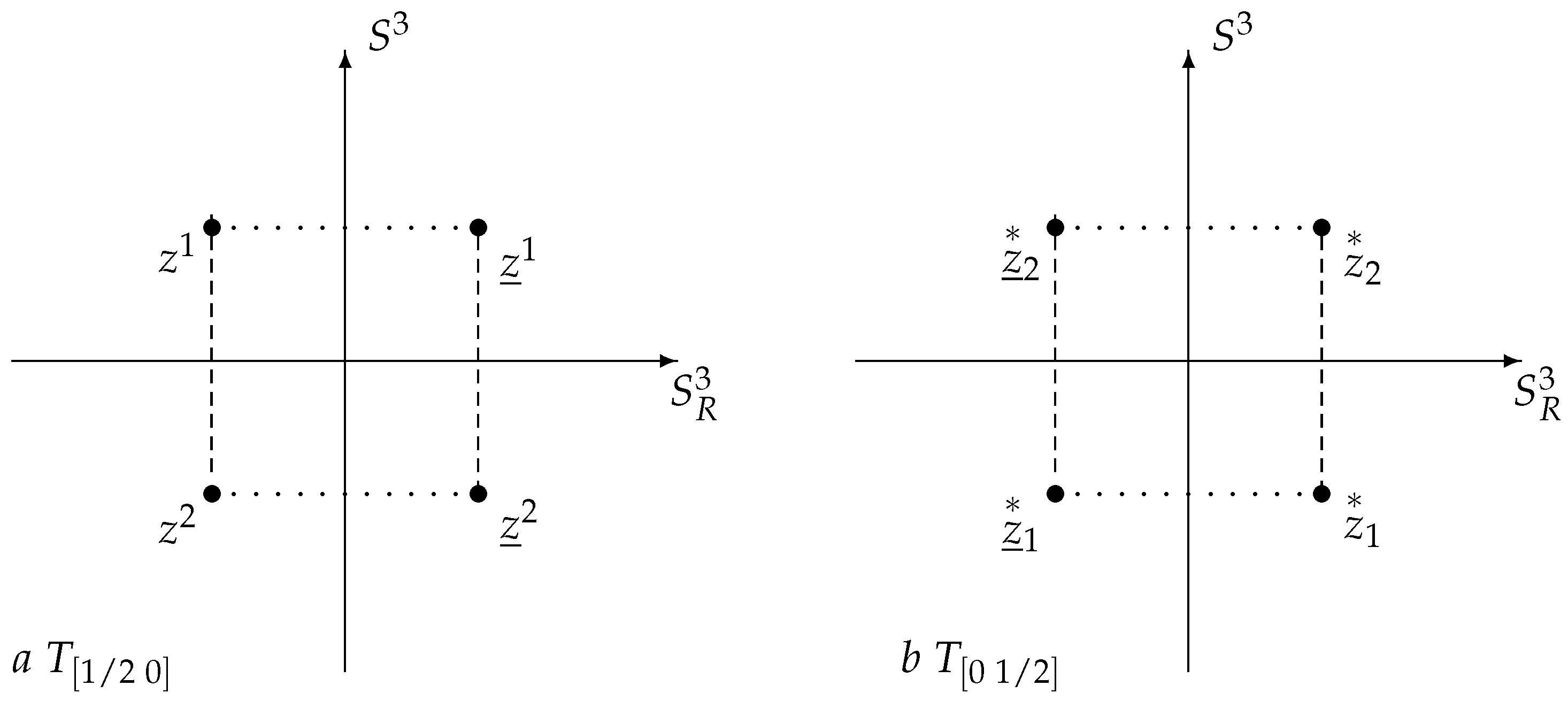
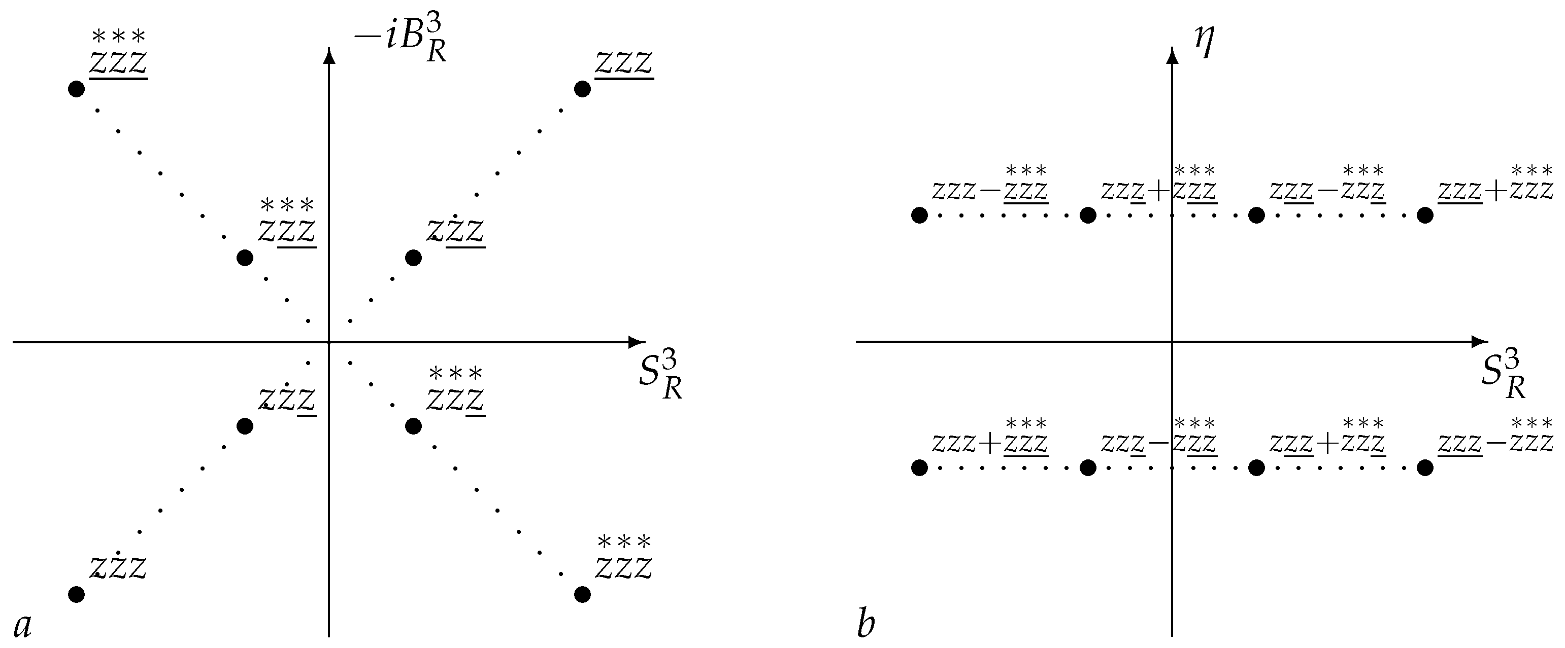
6.2. ${\mathit{j}}_{\mathbf{1}}+{\mathit{j}}_{\mathbf{2}}=\mathbf{1}/\mathbf{2}$, Spin 1/2

Consider the representations $T_{\left[{\displaystyle \frac{1}{2}}0\right]}$ and $T_{\left[0{\displaystyle \frac{1}{2}}\right]}$. The spin $S=1/2$, in the rest frame

$$\begin{array}{ccc}\hfill & S_R^3=-1/2& S_R^3=1/2\\ \eta =1\hfill & e^{-im{x}^0}(z^{\alpha }-{\stackrel{*}{\underline{z}}}_{\dot{\alpha }})& e^{-im{x}^0}({\underline{z}}^{\alpha }+{\stackrel{*}{z}}_{\dot{\alpha }})\\ \eta =-1\hfill & e^{-im{x}^0}(z^{\alpha }+{\stackrel{*}{\underline{z}}}_{\dot{\alpha }})& e^{-im{x}^0}({\underline{z}}^{\alpha }-{\stackrel{*}{z}}_{\dot{\alpha }})\end{array}$$

(40)

Each of the four functions corresponds to a point in Figure 2b. The different signs of the spin projection $S^3=\pm 1/2$ correspond to two possible values of the index $\alpha$ in Equation (40).

There are eight states, four particles; the particle states in the rest frame differ by their two possible spin projections.

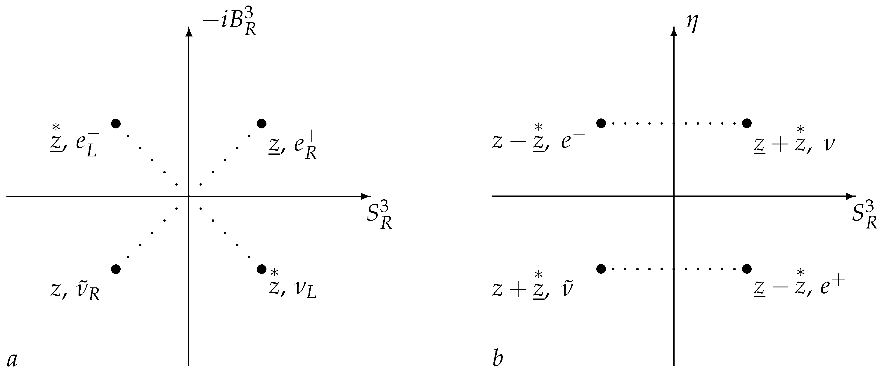
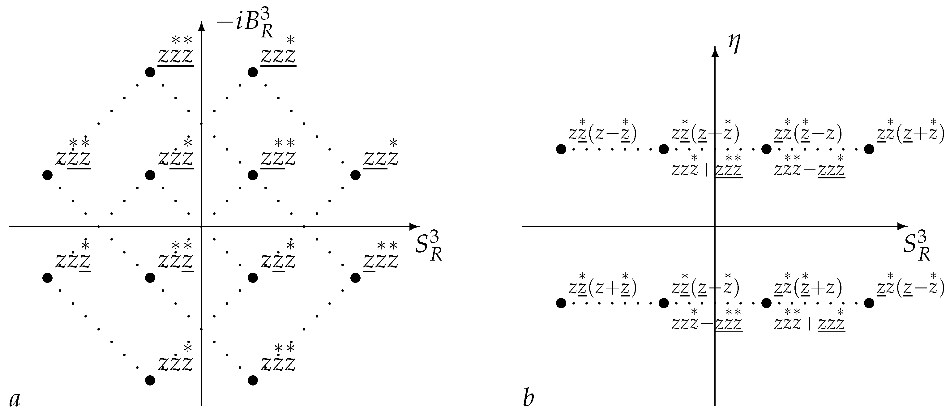
6.3. ${\mathit{j}}_{\mathbf{1}}+{\mathit{j}}_{\mathbf{2}}=\mathbf{1}$, Spin 1

The representations $T_{\left[10\right]}$ and $T_{\left[01\right]}$ are connected by space reflection, $S=j_1+j_2=1$. Each point in Figure 3b corresponds to three states with different spin projections.

$$\begin{array}{cccc}\hfill & S_R^3=-1& S_R^3=0& S_R^3=1\\ \eta =\pm 1\hfill & e^{-im{x}^0}(z^{\alpha }{z}^{\beta }\pm {\stackrel{*}{\underline{z}}}_{\dot{\alpha }}{\stackrel{*}{\underline{z}}}_{\dot{\beta }})& e^{-im{x}^0}(z^{(\alpha }{\underline{z}}^{\beta )}\mp {\stackrel{*}{z}}_{(\dot{\beta }}{\stackrel{*}{\underline{z}}}_{\dot{\alpha })})& e^{-im{x}^0}({\underline{z}}_{\alpha }{\underline{z}}_{\beta }\pm {\stackrel{*}{z}}_{\dot{\alpha }}{\stackrel{*}{z}}_{\dot{\beta }})\end{array}$$

(41)

Here, the parentheses around the indices indicate symmetrization.

There are 18 states, three particles; the particle states differ by parity $\eta =\pm 1$ and by three possible spin projection values in the rest frame.

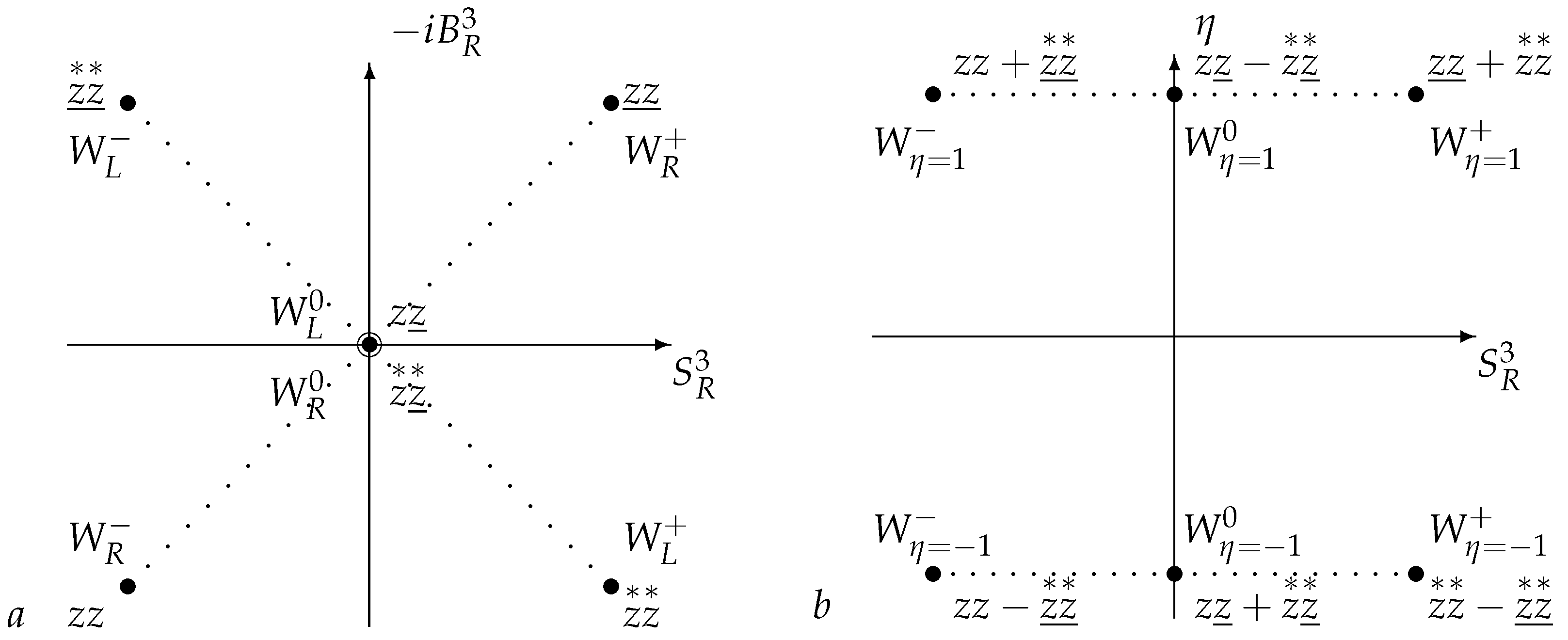
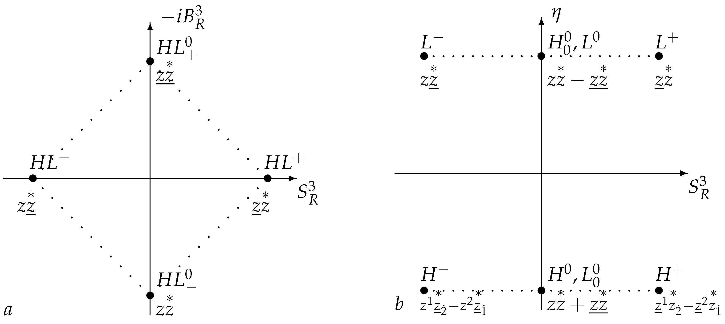
6.4. ${\mathit{j}}_{\mathbf{1}}+{\mathit{j}}_{\mathbf{2}}=\mathbf{1}$, Spin 0 and 1

The representation $T_{\left[{\displaystyle \frac{1}{2}}{\displaystyle \frac{1}{2}}\right]}$, 16 states in total. The four-dimensional representation, when reduced to a compact subgroup, decomposes into a scalar $(S=0)$ and a vector $(S=1)$.

For $S=0$, we have four particles, a singlet $H_0^0$, and a triplet $H^{-},H^0,H^{+}$ with respect to $SU{\left(2\right)}_{int}$. In the rest frame,

$$\begin{array}{cccc}\hfill & S_R^3=-1& S_R^3=0& S_R^3=1\\ S^R=1\hfill & e^{-im{x}^0}(z^1{\stackrel{*}{\underline{z}}}^{\dot{1}}+z^2{\stackrel{*}{\underline{z}}}^{\dot{2}})& e^{-im{x}^0}(z^1{\stackrel{*}{z}}^{\dot{1}}+z^2{\stackrel{*}{z}}^{\dot{2}}-{\underline{z}}^1{\stackrel{*}{\underline{z}}}^{\dot{1}}-{\underline{z}}^2{\stackrel{*}{\underline{z}}}^{\dot{2}})& e^{-im{x}^0}({\underline{z}}^1{\stackrel{*}{z}}^{\dot{1}}+{\underline{z}}^2{\stackrel{*}{z}}^{\dot{2}})\\ S^R=0\hfill & & e^{-im{x}^0}(z^1{\stackrel{*}{z}}^{\dot{1}}+z^2{\stackrel{*}{z}}^{\dot{2}}+{\underline{z}}^1{\stackrel{*}{\underline{z}}}^{\dot{1}}+{\underline{z}}^2{\stackrel{*}{\underline{z}}}^{\dot{2}})& \end{array}$$

(42)

Scalars represent the quadruplet of $SL{(2,C)}_{int}$. When reduced to the compact subgroup $SU{\left(2\right)}_{int}$, they split into a triplet $H^{-},H^0,H^{+}$ and a singlet $H_0^0$ (see Figure 4b). In the triplet $S_R^3=-1,0,+1$, corresponding—according to the empirical formula (25)—to the same values of electrical charge. With respect to the operator ${\hat{M}}_k$ algebra (see A7), the scalars form two doublets, $H^{-},H_{-}^0$ and $H_{+}^0,H^{+}$ (see Figure 4a).

We note that quantum numbers of the $H_0^0$ state (zero electric charge and the parity $\eta =1$) coincide with those of the Higgs boson.

For $S=1$, we also have four particles, a singlet $L_0^0$ and a triplet $L^{-},L^0,L^{+}$ with respect to $SU{\left(2\right)}_{int}$.

$$\begin{array}{cccc}\hfill & S^3=-1& S^3=0& S^3=1\\ L^{-},S_R^3=-1\hfill & e^{-im{x}^0}{z}^1{\stackrel{*}{\underline{z}}}^{\dot{2}}& e^{-im{x}^0}(z^1{\stackrel{*}{\underline{z}}}^{\dot{1}}-z^2{\stackrel{*}{\underline{z}}}^{\dot{2}})& e^{-im{x}^0}{z}^2{\stackrel{*}{\underline{z}}}^{\dot{1}}\\ L^{+},S_R^3=1\hfill & e^{-im{x}^0}{\stackrel{*}{z}}^1{\underline{z}}^{\dot{2}}& e^{-im{x}^0}({\stackrel{*}{z}}^1{\underline{z}}^{\dot{1}}-z^2{\stackrel{*}{\underline{z}}}^{\dot{2}})& e^{-im{x}^0}{\stackrel{*}{z}}^2{\underline{z}}^{\dot{1}}\\ L^0,S_R^3=0\hfill & e^{-im{x}^0}(z^1{\stackrel{*}{z}}^{\dot{2}}-{\underline{z}}^1{\stackrel{*}{\underline{z}}}^{\dot{2}})& e^{-im{x}^0}(z^1{\stackrel{*}{z}}^{\dot{1}}-z^2{\stackrel{*}{z}}^{\dot{2}}+{\underline{z}}^1{\stackrel{*}{\underline{z}}}^{\dot{1}}-{\underline{z}}^2{\stackrel{*}{\underline{z}}}^{\dot{2}})& e^{-im{x}^0}(z^2{\stackrel{*}{z}}^{\dot{1}}-{\underline{z}}^2{\stackrel{*}{\underline{z}}}^{\dot{1}})\\ L_0^0,S_R^3=0\hfill & e^{-im{x}^0}(z^1{\stackrel{*}{z}}^{\dot{2}}+{\underline{z}}^1{\stackrel{*}{\underline{z}}}^{\dot{2}})& e^{-im{x}^0}(z^1{\stackrel{*}{z}}^{\dot{1}}-z^2{\stackrel{*}{z}}^{\dot{2}}-{\underline{z}}^1{\stackrel{*}{\underline{z}}}^{\dot{1}}+{\underline{z}}^2{\stackrel{*}{\underline{z}}}^{\dot{2}})& e^{-im{x}^0}(z^2{\stackrel{*}{z}}^{\dot{1}}+{\underline{z}}^2{\stackrel{*}{\underline{z}}}^{\dot{1}})\end{array}$$

(43)

The case $S_R^3=0$ (fields $L^0$, $L_0^0$) corresponds to a truly neutral hypothetical particle, which is called the notoph in the literature [31,32,33] (in this case, the corresponding potentials are tensors transforming according to the representations $T_{\left[10\right]}$ and $T_{\left[01\right]}$).

Thus, just eight particles (states not connected by transformations $SL{(2,C)}_{ext}$) are associated with the representation $T_{{\displaystyle \frac{1}{2}}}\times T_{{\displaystyle \frac{1}{2}}}$.

The above can be summarized in Table 3. Each of the listed particles can be in several spin states; their number coincides with the dimension of the $SU{\left(2\right)}_{ext}$ representation.

Table 3. Classification of functions and their interpretation, $j_1+j_2\le 1$, $m\ne 0$.

Spin	$\mathit{\eta }$	$|{\mathit{j}}_1-{\mathit{j}}_2|$	Irreps of $\mathit{SL}{(\mathbf{2},\mathit{C})}_{\mathit{int}}$	Irreps of $\mathit{SU}{\left(\mathbf{2}\right)}_{\mathit{int}}\times \mathit{SU}{\left(\mathbf{2}\right)}_{\mathit{ext}}$ and Its Dimension		Dimension of $\mathit{SU}{\left(\mathbf{2}\right)}_{\mathit{int}}$ Irreps	Particles
${\displaystyle \frac{1}{2}}$	1	${\displaystyle \frac{1}{2}}$	$T_{\left[{\displaystyle \frac{1}{2}}0\right]},T_{[0,{\displaystyle \frac{1}{2}}]}$	$T_{{\displaystyle \frac{1}{2}}}\times T_{{\displaystyle \frac{1}{2}}}$	4	2	$e^{-},\nu$
${\displaystyle \frac{1}{2}}$	−1	${\displaystyle \frac{1}{2}}$	$T_{\left[{\displaystyle \frac{1}{2}}0\right]},T_{[0,{\displaystyle \frac{1}{2}}]}$	$T_{{\displaystyle \frac{1}{2}}}\times T_{{\displaystyle \frac{1}{2}}}$	4	2	$e^{+},\overline{\nu }$
1	±1	1	$T_{\left[10\right]},T_{[0,1]}$	$T_1\times T_1,$$T_1\times T_1$	18	3, 3	$W^{+},W^{-},W^0$
		0	$T_{\left[{\displaystyle \frac{1}{2}}{\displaystyle \frac{1}{2}}\right]}$		16
1	1	0		$T_1\times T_1$	9	3	$L^{+},L^{-},L^0$
1	−1	0		$T_1\times T_0$	3	1	$L^{00}$
0	−1	0		$T_0\times T_1$	3	3	$H^{+},H^0,H^{-}$
0	1	0		$T_0\times T_0$	1	1	$H^{00}$

6.5. ${\mathit{j}}_{\mathbf{1}}+{\mathit{j}}_{\mathbf{2}}=\mathbf{3}/\mathbf{2}$, Spin 1/2 and 3/2

The representations $T_{\left[{\displaystyle \frac{3}{2}}0\right]}$ and $T_{\left[0{\displaystyle \frac{3}{2}}\right]}$ are related by space reflection, $S=j_1+j_2=3/2$. There are 32 states in total and eight particles (states that are not connected by transformations $SL{(2,C)}_{int}$, differing by the values $S_R^3$$(\pm 1/2,\pm 3/2)$ and by the parity, corresponding to eight points in Figure 5b. Each point of the weight diagram (Figure 5b) corresponds to four states (according to the number of possible spin projections).

The representations $T_{\left[1{\displaystyle \frac{1}{2}}\right]}$ and $T_{\left[{\displaystyle \frac{1}{2}}1\right]}$ are related by a space reflection, $S=j_1+j_2=1$. There are 72 states in total. These are 12 spin $3/2$ particles, differing by the parity, by the values of $S_R$$(1/2,3/2)$ and $S_R^3$$(\pm 1/2,\pm 3/2)$, and 12 spin $1/2$ particles, differing by the parity, by the values of $S_R$$(1/2,3/2)$ and $S_R^3$$(\pm 1/2,\pm 3/2).$ The above can be summarized in Table 4.

Table 4. Classification of scalar functions, $j_1+j_2=3/2$, $m\ne 0$.

Spin	$\mathit{\eta }$	$|{\mathit{j}}_1-{\mathit{j}}_2|$	Irreps of $\mathit{SL}{(\mathbf{2},\mathit{C})}_{\mathit{int}}$	Irreps of $\mathit{SU}{\left(\mathbf{2}\right)}_{\mathit{int}}\times \mathit{SU}{\left(\mathbf{2}\right)}_{\mathit{ext}}$ and Its Dimension		Dimension of $\mathit{SU}{\left(\mathbf{2}\right)}_{\mathit{int}}$ Irreps
3/2	±1	${\displaystyle \frac{3}{2}}$	$T_{\left[{\displaystyle \frac{3}{2}}0\right]},T_{[0,{\displaystyle \frac{3}{2}}]}$	$T_{{\displaystyle \frac{3}{2}}}\times T_{{\displaystyle \frac{3}{2}}},T_{{\displaystyle \frac{3}{2}}}\times T_{{\displaystyle \frac{3}{2}}}$	32	4, 4
		${\displaystyle \frac{1}{2}}$	$T_{\left[{\displaystyle \frac{3}{2}}{\displaystyle \frac{1}{2}}\right]},T_{\left[{\displaystyle \frac{1}{2}}{\displaystyle \frac{3}{2}}\right]}$		72
3/2	1			$T_{{\displaystyle \frac{3}{2}}}\times T_{{\displaystyle \frac{3}{2}}},T_{{\displaystyle \frac{3}{2}}}\times T_{{\displaystyle \frac{3}{2}}}$	36	4, 4
3/2	−1			$T_{{\displaystyle \frac{3}{2}}}\times T_{{\displaystyle \frac{1}{2}}},T_{{\displaystyle \frac{3}{2}}}\times T_{{\displaystyle \frac{1}{2}}}$	16	2, 2
1/2	−1			$T_{{\displaystyle \frac{1}{2}}}\times T_{{\displaystyle \frac{3}{2}}},T_{{\displaystyle \frac{1}{2}}}\times T_{{\displaystyle \frac{3}{2}}}$	16	4, 4
1/2	1			$T_{{\displaystyle \frac{1}{2}}}\times T_{{\displaystyle \frac{1}{2}}},T_{{\displaystyle \frac{1}{2}}}\times T_{{\displaystyle \frac{1}{2}}}$	8	2, 2

7. The Ultra-Relativistic Limit

Let us consider a massive particle, moving along the axis $x^3$. Corresponding functions $f(x,z)$ can be obtained from functions in the rest frame by means of a Lorentz transformation $U\in SL(2,C)$,

$$\begin{array}{ccc}& & P=U{P}_0{U}^{†},Z=U{Z}_0,P_0=\mathrm{diag}\{m,m\},U=\mathrm{diag}\{e^a,e^{-a}\},\hfill \\ & & p_0=mcosh2a,p_3=msinh2a,e^{\pm a}=\sqrt{(p_0\pm p_3)/m}.\hfill \end{array}$$

(44)

For the orientation variables, we have the following:

$$(z^1,{\underline{z}}^1,{\stackrel{*}{z}}_2,{\stackrel{*}{\underline{z}}}_2)\to e^a(z^1,{\underline{z}}^1,{\stackrel{*}{z}}_2,{\stackrel{*}{\underline{z}}}_2),(z^2,{\underline{z}}^2,{\stackrel{*}{z}}_1,{\stackrel{*}{\underline{z}}}_1)\to e^{-a}(z^2,{\underline{z}}^2,{\stackrel{*}{z}}_1,{\stackrel{*}{\underline{z}}}_1).$$

If we apply these transformations to functions (40)–(43) and consider the ultra-relativistic limit, then only states for which helicity is equal to chirality will remain in it.

For example, applying these transformations to the state with $S_R^3=-1/2$, $\eta =1$ from (40), we find

$$\begin{array}{ccc}\hfill f(x,z)& \to & f^{\prime }(x,z)=e^{i(k_0{x}^0+k_3{x}^3)}\left(C_1(z^1{e}^a-{\stackrel{*}{\underline{z}}}_{\dot{1}}{e}^{-a})\right.+\left.C_2(z^2{e}^{-a}-{\stackrel{*}{\underline{z}}}_{\dot{2}}{e}^a)\right),\hfill \end{array}$$

(45)

where the first term corresponds to $S^3=1/2$, and the second term corresponds to $S^3=-1/2$. In the ultra-relativistic case with a positive a ($k_3>0$), there remain only two components:

$$f^{\prime }(x,z)\approx e^{i(k_0{x}^0+k_3{x}^3)}\left(C_1{z}^1{e}^a-C_2{\stackrel{*}{\underline{z}}}_{\dot{2}}{e}^a\right).$$

(46)

The first term corresponds to $S^3>0$ and chirality $\lambda =1/2$; the second term corresponds to $S^3<0$ and chirality $\lambda =-1/2$. We see that in the ultra-relativistic limit with $p_0>0$, the signs of chirality and helicity $\hat{\mathbf{p}}\hat{\mathbf{S}}$ are the same.

As should be expected, the results of this analysis of the ultra-relativistic case coincide with the conclusions on the chirality and helicity of a particle with spin 1/2, obtained on the basis of the Dirac equation.

For states (41) of spin 1 (representations of $T_{\left[10\right]}$ and $T_{\left[01\right]}$), only two terms remain in the ultra-relativistic limit—those with the same signs of helicity and chirality.

For states (43) of spin 1 (representation $T_{[{\displaystyle \frac{1}{2}},{\displaystyle \frac{1}{2}}]}$), only one term remains in the ultra-relativistic limit: the one with $S^3=0$ and zero chirality.

8. First-Order Left-Invariant Equations

In the case of massless particles, first-order equations in ${\hat{p}}^{\mu }$ appear within the framework of the classification of functions with respect to the irreps of the Poincaré group. In contrast, for massive particles, we have two second-order eigenvalue equations for the Casimir operators ${\hat{\mathit{p}}}^2$ and ${\hat{\mathit{W}}}^2$. For massive particles, it is impossible to construct first-order equations using only the generators of the Poincaré group. The desired equations must be invariant under the transformations $M{(3,1)}_{ext}$ and, for particles with a certain parity, also under space reflection. In this case, invariance with respect to $M{(3,1)}_{int}$ is not required; internal symmetries can be broken.

From the orientation variables z, one can construct operators that are transformed as vectors with respect to $M{(3,1)}_{ext}$ and $M{(3,1)}_{int}$, preserving the degree of polynomials in z (see Ref. [19]) as follows:

$$\begin{array}{ccc}\hfill {\hat{\Gamma }}^{\mu \underline{n}}& =& {\displaystyle \frac{1}{2}}\left({\overline{\sigma }}^{\mu \dot{\alpha }\beta }{\sigma }_{\underline{b}\dot{\underline{a}}}^{\underline{n}}{\stackrel{*}{z}}_{\dot{\alpha }}^{\dot{\underline{a}}}{\partial }_{\beta }^{\underline{b}}+{\sigma }_{\beta \dot{\alpha }}^{\mu }{\overline{\sigma }}^{\underline{n}\dot{\underline{a}}\underline{b}}{z}_{\underline{b}}^{\beta }{\partial }_{\dot{\underline{a}}}^{\dot{\alpha }}\right),\hfill \end{array}$$

(47)

$$\begin{array}{ccc}\hfill \hat{\underline{\Gamma }}{\phantom{\Gamma }}^{\mu \underline{n}}& =& {\displaystyle \frac{1}{2}}\left({\overline{\sigma }}^{\mu \dot{\alpha }\beta }{\sigma }_{\underline{b}\dot{\underline{a}}}^{\underline{n}}{\stackrel{*}{z}}_{\dot{\alpha }}^{\dot{\underline{a}}}{\partial }_{\beta }^{\underline{b}}-{\sigma }_{\beta \dot{\alpha }}^{\mu }{\overline{\sigma }}^{\underline{n}\dot{\underline{a}}\underline{b}}{z}_{\underline{b}}^{\beta }{\partial }_{\dot{\underline{a}}}^{\dot{\alpha }}\right),\hfill \end{array}$$

(48)

with one external (left) and one internal (right) index. Only the operators ${\hat{p}}_{\mu }{\hat{\Gamma }}^{\mu \underline{0}}$ and ${\hat{p}}_{\mu }\hat{\underline{\Gamma }}{\phantom{\Gamma }}^{\mu \underline{k}}$, $\underline{k}=1,2,3$ are invariant under the space reflection, and the associated four equations possess solutions with a definite inner parity.

Let us consider the following equation:

$${\hat{p}}^{\mu }{\hat{\Gamma }}^{\mu \underline{0}}f(x,z)={\varkappa }^{\underline{0}}f(x,z),$$

(49)

where

$$\begin{array}{ccc}\hfill 2{\hat{\Gamma }}^{\mu \underline{0}}& =& {\overline{\sigma }}^{\mu \dot{\alpha }\beta }({\stackrel{*}{z}}_{\dot{\alpha }}^{\dot{\underline{1}}}{\partial }_{\beta }^{\underline{1}}+{\stackrel{*}{z}}_{\dot{\alpha }}^{\dot{\underline{2}}}{\partial }_{\beta }^{\underline{2}})+{\sigma }_{\beta \dot{\alpha }}^{\mu }(z_{\underline{1}}^{\beta }{\partial }_{\dot{\underline{1}}}^{\dot{\alpha }}+z_{\underline{2}}^{\beta }{\partial }_{\dot{\underline{2}}}^{\dot{\alpha }})\hfill \\ & =& ({\overline{\sigma }}^{\mu \dot{\alpha }\beta }{\stackrel{*}{\underline{z}}}_{\dot{\alpha }}\partial /\partial z^{\beta }+{\sigma }_{\beta \dot{\alpha }}^{\mu }{z}^{\beta }\partial /\partial {\stackrel{*}{\underline{z}}}_{\dot{\alpha }})+({\overline{\sigma }}^{\mu \dot{\alpha }\beta }{\stackrel{*}{z}}_{\dot{\alpha }}\partial /\partial {\underline{z}}^{\beta }+{\sigma }_{\beta \dot{\alpha }}^{\mu }{\underline{z}}^{\beta }\partial /\partial \stackrel{*}{\phantom{z}}{z}_{\dot{\alpha }}).\hfill \end{array}$$

(50)

The set of the operators ${\hat{S}}^{\mu \nu }$ and ${\hat{\Gamma }}^{\mu \underline{0}}$ satisfies the commutation relations of the group $SO(3,2)$.

Obviously, Equation (49) is not invariant under right boosts, since the operator ${\hat{p}}_{\mu }{\hat{\Gamma }}^{\mu \underline{0}}$ does not commute with a part of the right generators, namely with $\hat{\mathbf{S}}\hat{\mathbf{B}}$, ${\hat{B}}_R^3$, and $p_{\mu }^R$. However, it commutes with ${\hat{\mathbf{S}}}^2-{\hat{\mathbf{B}}}^2$ and with generator $S_R^3$ of $SU{\left(2\right)}_{int}$, which is why particles described by Equation (49) may have certain values of $j_1+j_2$ and $S_R^3$. And if the parity operator connects only states with different signs of $j_1-j_2$, then the operator ${\hat{p}}_{\mu }{\hat{\Gamma }}^{\mu }$ connects states with all possible values of $j_1$ and $j_2$ for a fixed sum $j_1+j_2$.

Thus, the invariant subspaces of the operators ${\hat{\Gamma }}^{\mu \underline{0}}$ are subspaces of polynomials of degree $2(j_1+j_2)$ by z with fixed values of $S_R^3$. In particular, such subspaces are the spaces of polynomials $f(x,z,\stackrel{*}{\underline{z}})$ and $f(x,\underline{z}\phantom{z},\stackrel{*}{z})$ of degree $2(j_1+j_2)$, characterized by $S_R^3=\mp (j_1+j_2)$.

Let us take a closer look at the case of spin 1/2. Linear functions from the subspace $f(x,z,\stackrel{*}{\underline{z}})$ depend on four variables $z^{\alpha },{\stackrel{*}{\underline{z}}}_{\dot{\alpha }}$, $S_R^3=-1/2$. For them, we have two equations of the form (49) with different signs of the mass term. Each of these two equations combines two irreps of the improper Poincaré group, characterized by the same sign of $p_0\eta$. One can see that in the rest frame,

$${\varkappa }^{\underline{0}}=\epsilon ms,\epsilon =\eta \mathrm{sign}{p}_0\mathrm{sign}{S}_R^3.$$

(51)

In total, for functions linear in orientation variables, we have four equations; their solutions in the rest frame at $p_0>0$ are given by the formulas in (40). Although the particle and its antiparticle belong to different subspaces with $S_R^3=\pm 1/2$, they are described by equations with the same sign before the mass term.

Let us introduce the generator of the group $U\left(1\right)$ corresponding to phase transformations of orientation variables z:

$${\hat{\Gamma }}^5=\frac{1}{2}\left(z_{\underline{a}}^{\alpha }{\partial }_{\alpha }^{\underline{a}}-{\stackrel{*}{z}}_{\dot{\underline{b}}}^{\dot{\beta }}{\partial }_{\dot{\beta }}^{\dot{\underline{b}}}\right).$$

(52)

These transformations, along with external and internal automorphisms of the Poincaré group, can be considered as field symmetry transformations on the Poincaré group; see Ref. [19]. Polynomials of degree n in $z,\underline{z}$ and of degree m in $\stackrel{*}{z},\stackrel{*}{\underline{z}}\phantom{z}$ are eigenfunctions of the operator ${\hat{\Gamma }}^5$ with the eigenvalue $n-m$. In the subspaces of the functions $f(x,z,\stackrel{*}{\underline{z}})$ and $f(x,\underline{z},\stackrel{*}{z})$, its eigenvalues coincide with the chirality, defined as $j_1-j_2$. The chirality operator ${\Gamma }^5$ commutes with the right and the left generators of the Poincaré group but does not commute with ${\Gamma }^{\mu \underline{0}}$.

The matrix representation of the Dirac equation can be obtained from Equation (49) for the functions $f(x,z,\stackrel{*}{\underline{z}})$ and $f(x,\underline{z},\stackrel{*}{z})$, which are polynomials of the first order in z.

For example, substituting functions linear in z, corresponding to the spin $1/2$ from the subspace $f(x,z,\stackrel{*}{\underline{z}})$,

$$\begin{array}{ccc}& & f_D(x,z)={\chi }_{\alpha }\left(x\right)z^{\alpha }+{\stackrel{*}{\psi }}^{\dot{\alpha }}\left(x\right){\stackrel{*}{\underline{z}}}_{\dot{\alpha }}=Z_D{\Psi }_D\left(x\right),\hfill \\ & & Z_D=\left(z^{\alpha }{\stackrel{*}{\underline{z}}}_{\dot{\alpha }}\right),{\Psi }_D\left(x\right)=\left({\displaystyle \genfrac{}{}{0pt}{}{{\chi }_{\alpha }\left(x\right)}{{\stackrel{*}{\psi }}^{\dot{\alpha }}\left(x\right)}}\right),\hfill \end{array}$$

(53)

into Equation (49) and making a comparison of the coefficients at $z^{\alpha }$ and ${\stackrel{*}{\underline{z}}}_{\dot{\alpha }}$ in the left- and right-hand sides, we obtain the Dirac equation:

$$({\hat{p}}_{\mu }{\gamma }^{\mu }-\varkappa ){\Psi }_D\left(x\right)=0,$$

(54)

where $\varkappa =2{\varkappa }^{\underline{0}}$. The action of the chirality operator (52) amounts to the multiplication by ${\gamma }^5/2$, ${\gamma }^5=\mathrm{diag}\{{\sigma }^0,-{\sigma }^0\}$,

$${\hat{\Gamma }}^5{f}_D(x,z)={\displaystyle \frac{1}{2}}{Z}_D{\gamma }^5{\Psi }_D\left(x\right).$$

Similarly, considering polynomials of the second degree leads to the 10-component Duffin–Kemmer equations, while higher-degree polynomials lead to the Bhabha equations. Note that starting with second-order polynomials in z, states of the form (41) transforming according to representations of $T_{\left[j0\right]}$ or $T_{\left[0j\right]}$ are not, generally speaking, eigenfunctions of ${\hat{p}}^{\mu }{\hat{\Gamma }}^{\mu \underline{0}}$, and in the rest frame, solutions of these equations contain components that transform according to other representations.

9. Discussion and Conclusions

A classification of relativistic orientable objects and its connection to particle phenomenology is studied. This study is based on the possibility of describing these objects by a scalar field on the Poincaré group. Scalar functions $f\left(q\right)$, $q=(x,z)$, on the group depend on the Minkowski space coordinates $x=\left(x^{\mu }\right)=\left(x^0,\mathbf{x}\right),$ $\mathbf{x}=\left(x^k\right),$ as well as on the orientation variables $z=\left(z_{\alpha \beta }\right)$ given by elements of the matrix $Z\in SL(2,C)$. The functions have certain transformation properties with respect to both groups $M{(3,1)}_{ext}$ and $M{(3,1)}_{int}$; see Section 1. We classify them with the help of maximal sets of commuting operators constructed from generators of the groups $M{(3,1)}_{ext}$ and $M{(3,1)}_{int}$.

We suppose that different particles correspond to states described by functions $f(x,z)$ that are not connected by transformations from $M{(3,1)}_{ext}$ (i.e., by a change in the space-fixed reference frame). Such states are classified by eigenvalues of Casimir operators and some functions of the right generators of the group (i.e., generators of the group $M{(3,1)}_{int}$).

This way of classification, applied to linear and quadratic functions of z, allows one to identify some of them with known elementary particles of spin 0, ${\displaystyle \frac{1}{2}}$, and 1. Below, we list the results of such an identification (the enumeration is given by values of spin and chirality in the massless limit).

Spin 1/2, chirality $\pm \mathbf{1}/\mathbf{2}$. Such particles appear in quadruplets, but not in particle/antiparticle pairs.

In the massless case, we have four states and four particles—two $SL{(2,C)}_{int}$ doublets of chirality $\lambda =-1/2$ (particles) and $\lambda =-1/2$ (their antiparticles), interconnected by both space reflection and charge conjugation. The particle and the antiparticle differ in charge signs $S_R^3$, with each of them appearing in one chiral state only. When reduced to $SU{\left(2\right)}_{int}\subset SL{(2,C)}_{int}$, these two-dimensional representations remain irreducible.

In the real world, the four fundamental fermions (in massless limit) have identical properties, for example, $(e_L^{-},{\nu }_L)$ and $(e_R^{+},{\tilde{\nu }}_R)$ or $(d_L,u_L)$ and $({\tilde{d}}_R,{\tilde{u}}_R)$.

In the massive case, we have eight states and four particles, differing in sign $S_R^3$ and parity ($\eta =1$ corresponds to particles and $\eta =-1$ corresponds to antiparticles). In the rest frame, states of one particle differ by two spin projections $S_3=\pm 1/2$. The fours $(e^{-},\nu )$ and $(e^{+},\tilde{\nu })$ or $(d,u)$ and $(\tilde{d},\tilde{u})$ of fundamental fermions have analogous properties, excluding the equality of masses.

Spin 1, chirality $\pm \mathbf{1}$.

In the massless case, there appear six states and six particles: two $SO{(3,C)}_{int}\sim SL{(2,C)}_{int}$ triplets of chirality $\lambda =-1$ (particles) and $\lambda =1$ (antiparticles), interconnected by both space reflection and charge conjugation. Components of the triplets differ in charge $S_R^3=0,\pm 1$; each particle is in only one chiral state. When reduced to $SU{\left(2\right)}_{int}\subset SL{(2,C)}_{int}$, these three-dimensional representations remain irreducible.

In the massive case, we have 18 states and six particles, differing in quantum numbers $S_R^3=0,\pm 1$ and in parity, $\eta =1$ (three particles) and $\eta =-1$ (three antiparticles). In the rest frame, the states of one particle differ by three projections of spin, $S_3=0,\pm 1$.

These two triples differ only in the signs of chirality ($m=0$) or parity ($m\ne 0$). Therefore, if it turns out that the other charges of such particles are the same, then they can be considered as different polarization states of one particle. Under this interpretation, we have one triplet, each component of which has two ($m=0$) or six states ($m\ne 0$).

The triplet $(W^{-},W^0,W^{+})$ of vector bosons (in massless limit) has identical properties with the one considered above. In the massive case, the triplet $(W^{-},Z^0,W^{+})$ has similar properties, excluding the equality of masses.

Spin 1, chirality $\mathbf{0}$.

In the case $m\ne 0$, we have an $SO{(3,1)}_{int}\sim SL{(2,C)}_{int}$ quadruplet of particles, containing two truly neutral particles ($\eta =\pm 1$, $S_R^3=0$) and two charged particles ($\eta =1$, $S_R^3=\pm 1$). Each particle from the quadruplet can be in three states, which differ in the rest frame by three projections of the spin $S_3=0,\pm 1$. In the ultra-relativistic limit, there remains only one state with zero projection of the spin on the direction of motion.

The case $S_R^3=0$ corresponds to a truly neutral hypothetical particle, which is called the notoph in the literature.

Chirality $\mathbf{0}$. In the massless case, the $SO{(3,1)}_{int}\sim SL{(2,C)}_{int}$ quadruplet of particles contains two truly neutral particles ($S_R^3=0$), differing by the values of $B_3^R$, and two charged particles ($S_R^3=\pm 1$). Each particle from the quadruplet has only one chiral state with zero projection of the spin on the direction of motion.

Spin 0. Scalar particles are represented by a singlet (independent of z functions $f\left(x\right)$) and a quadruplet (second-order polynomials in z). The quadruplet consists of two truly neutral particles ($\eta =\pm 1$, $S_R^3=0$) and two charged particles ($\eta =-1$, $S_R^3=\pm 1$). The characteristics of the Higgs boson correspond to both the singlet and to the component of the quadruplet with $\eta =1$.

This list exhausts orientable objects described by polynomials of the zeroth, first, and second orders in orientation variables.

Among the states discussed above, there exist states with the same $S_R^3$ that differ only by signs of the chirality (or parity, for $m\ne 0$). This raises the question: should these states be interpreted as describing different particles, or merely different polarization states of one and the same particle? If we start only from the representation theory of the Poincaré group, we do not obtain any answer to such a question. But using the empirical formula (25), we see that in the case of spin 1/2, these states differ in the electric charge and, therefore, are states of different particles (electron and neutrino). At the same time, in the case of spin 1, Equation (25) does not prohibit interpreting them as different polarization states of one and the same particle (photon, W bosons).

When considering relativistic wave equations and particles described by them, only 8 out of 10 from the maximal set of commuting operators of the Poincaré group are usually used (six left generators and two of four functions of the right generators, with the latter defining the irrep of the Lorentz group $SL{(2,C)}_{int}$). Here, for the classification of the orientable objects, we have used all 10 operators from the maximal set.

We stress that the results of the developed classification do not contradict the phenomenology of elementary particles and, moreover, in some cases, present the corresponding group-theoretic explanation. In addition, the relationship between the spectra of the left and right generators allows us to give a possible explanation of the relationship between spin and the internal quantum numbers (charges) of particles, expressed in the positivity of R-parity.

In addition, it seems important to note that the composition and properties of particles predicted by the presented classification follow exclusively from the properties of the space–time and are, in a sense, model-independent.