Abstract
Solar flares are significant occurrences in solar physics, impacting space weather and terrestrial technologies. Accurate classification of solar flares is essential for predicting space weather and minimizing potential disruptions to communication, navigation, and power systems. This study addresses the challenge of selecting the most relevant features from multivariate time-series data, specifically focusing on solar flares. We employ methods such as Mutual Information (MI), Minimum Redundancy Maximum Relevance (mRMR), and Euclidean Distance to identify key features for classification. Recognizing the performance variability of different feature selection techniques, we introduce an ensemble approach to compute feature weights. By combining outputs from multiple methods, our ensemble method provides a more comprehensive understanding of the importance of features. Our results show that the ensemble approach significantly improves classification performance, achieving values 0.15 higher in True Skill Statistic (TSS) values compared to individual feature selection methods. Additionally, our method offers valuable insights into the underlying physical processes of solar flares, leading to more effective space weather forecasting and enhanced mitigation strategies for communication, navigation, and power system disruptions.
1. Introduction
Space weather refers to the environmental conditions in space as influenced by the Sun and the solar wind. These conditions can significantly impact technological systems and human activities on Earth and in space. One of the primary drivers of space weather is solar flares, which are sudden bursts of electromagnetic radiation emanating from the Sun’s surface. Solar flares can be observationally defined as a brightening of any emission across the electromagnetic spectrum occurring from minutes to hours. Most manifestations appear to be secondary responses to the initial energy release process, converting magnetic energy into particle energy, heat, waves, and motion [1]. Solar flares occur when magnetic energy that has built up in the solar atmosphere is suddenly released, causing a brightening in extreme ultraviolet (EUV) and X-ray emissions. These events can last a few minutes to several hours [2].
Solar flares play a crucial role in space weather and are often accompanied by coronal mass ejections (CMEs), which are large expulsions of plasma and the magnetic field from the Sun’s corona [3]. When these flares and CMEs interact with the Earth’s magnetic field, they can induce geomagnetic storms characterized by disturbances in the Earth’s magnetosphere. These disturbances lead to various space weather phenomena such as auroras, disruptions in communication systems, and impacts on power grids [2]. The Sun’s magnetic activity, which drives solar flares and CMEs, can produce severe disturbances in the upper atmosphere and near-Earth space environment. Strong auroral currents induced by these disturbances can disrupt and damage modern electric power grids and contribute to the corrosion of oil and gas pipelines. Magnetic-storm-driven ionospheric density disturbances can interfere with high-frequency (HF) radio communications and navigation signals from Global Positioning System (GPS) satellites. During severe polar cap absorption (PCA) events, HF communications along transpolar aviation routes can be completely blacked out, necessitating aircraft to be diverted to lower latitudes. Additionally, the exposure of spacecraft to energetic particles during solar energetic particle events and radiation belt enhancements can cause temporary operational anomalies, damage critical electronics, degrade solar arrays, and impair optical systems such as imagers and star trackers [4,5,6].
A historical example of the profound impact of space weather is the Carrington event in 1859. This event is often regarded as the most significant space weather event recorded. Triggered by a massive solar flare observed by Richard Carrington and Richard Hodgson, it led to a significant geomagnetic storm that induced strong currents in telegraph systems worldwide, causing widespread communication disruptions [7]. A few years after Carrington and Hodgson’s observations, the Sun was studied extensively in the hydrogen H line originating in the chromosphere, and reports of flares became much more frequent but also bewilderingly complex [8]. A 2008 report by the National Research Council concluded that a solar superstorm similar to the 1859 Carrington event could cripple the entire US power grid for months, resulting in economic damages estimated between 1 to 2 trillion dollars [4].
Given the potential impacts of space weather, the development of reliable solar flare prediction models is crucial. However, the relationship between the photospheric and coronal magnetic fields during a solar flare is not fully understood. Flare prediction has thus far relied predominantly on classifiers that attempt to automatically find such relationships rather than purely theoretical considerations [9]. Machine learning, mainly supervised classifiers, has been employed to predict flares by identifying patterns in the magnetic field data. These linear or nonlinear classifiers attempt to segregate active regions into those likely to produce flares and those that are not, based on their magnetic characteristics [9]. Additionally, the goal is to predict, days in advance, the onset time, intensity, and duration of geomagnetic storms on Earth. These storms are characterized by a sudden injection of particles into the magnetosphere, causing a significant disturbance in the Earth’s magnetic field. The major contributor to intense geomagnetic storms is not solar flares, as commonly believed, but coronal mass ejections (CMEs) [3].
Feature selection for multivariate time-series (MVTS) classification is essential in handling high-dimensional datasets, such as those used for solar flare class prediction. Feature selection is critical in managing MVTS data, as it helps identify the most relevant features while removing redundant or irrelevant ones. Several methods have been proposed for effective feature selection. Mutual Information (MI) is one such method, known for its ability to measure the mutual dependence between variables. MI helps identify features that maximize the information shared with the target variable, enhancing classification results. Studies have shown that MI-based feature selection significantly improves the accuracy and effectiveness of classification models in solar flare class prediction [10]. Another effective method is Minimum Redundancy Maximum Relevance (mRMR), which balances the relevance and redundancy of features by selecting those that have the maximum relevance to the target variable while ensuring minimal redundancy among the selected features. This approach has proven effective in improving classification performance for time-series data, as it enhances the diversity and relevance of the selected features, thereby boosting the model’s ability to classify solar flares [11] accurately. Additionally, Euclidean Distance is used to rank features based on their separability. This method evaluates the distance between features to determine their importance, with higher distances ranked higher. By focusing on these highly separable features, the method improves classification results while reducing computational load. This approach has been particularly effective in high-dimensional datasets like those used for solar flare class prediction [12].
Various classifiers have been applied to the solar flare class prediction task, each offering unique strengths. Rocket and MiniRocket classifiers have shown significant promise in handling MVTS data. MiniRocket, in particular, has demonstrated superior performance compared to other classifiers like Long Short-Term Memory (LSTM), Fast Time-Series Classification with Symbolic Representations (Mr-SEQL), Support Vector Machine (SVM), and Canonical Interval Forest (CIF). Experimental findings indicate substantial improvements in the True Skill Statistic (TSS) and Heidke Skill Score (HSS2), highlighting the classifier’s capability to manage MVTS data complexities and improve space weather prediction results [13]. Random Forest is another classifier known for its robustness and ability to handle high-dimensional data effectively. It manages feature selection outputs efficiently and provides reliable classification results for solar flare occurrences. This ensemble learning method is valuable in space weather prediction due to its consistent performance and adaptability to various datasets [14,15].
Comparative studies underscore the effectiveness of different feature selection methods and classifiers [16]. For instance, research using the MiniRocket classifier for the SWAN-SF dataset showed consistent improvement in classification results over other classifiers, emphasizing the importance of excluding less significant flare classes (e.g., B- and C-class flares) to maximize performance [13]. Additionally, feature subset selection methods like MI, mRMR, and Euclidean Distance have been shown to outperform traditional methods such as Recursive Feature Elimination (RFE) and Fisher Criterion (FC) in terms of classification performance and computational efficiency [17,18].
This study introduces a novel ensemble feature selection method that combines Mutual Information, mRMR, and Euclidean Distance with classifiers such as MiniRocket, Rocket, and Random Forest. Our approach leverages consecutive data partitions to maintain temporal continuity, ensuring that the models are trained and tested in a manner that closely mimics real-world scenarios. This is the first attempt to perform feature selection without employing sampling techniques, thereby representing real-world scenarios more accurately. Through this methodology, we aim to provide a robust and comprehensive evaluation of the feature selection methods and classifiers, addressing the variability and uncertainty in the data.
2. Dataset
The Space-Weather ANalytics for Solar Flares (SWAN-SF) is an open access, comprehensive multivariate time-series dataset [19]. This dataset primarily utilizes data from the Solar Dynamics Observatory Helioseismic and Magnetic Imager (SDO/HMI) Active Region Patches (SHARPs) [20], managed by the Joint Science Operations Center (JSOC). It also includes Geostationary Operational Environmental Satellite (GOES) flare records, enhanced with additional data from Hinode-XRT to ensure precise flare location verification. Spanning from 1 May 2010 to 31 August 2018, the dataset is meticulously curated to provide high-quality inputs essential for solar flare prediction. Available through Harvard Dataverse [21], it comprises 4098 instances, each featuring 51 time-series parameters recorded at 12 min intervals. Of these, 24 parameters specifically relate to magnetic fields, crucial for understanding and predicting solar flare activities due to their significant role in magnetic reconnection processes [2]. Since solar flares are considered magnetic phenomena, accurately forecasting and classifying flares relies on the selection of appropriate magnetic field properties and prediction methods [22,23,24,25,26,27]. We focus on these 24 magnetic parameters, as shown in Table 1.

Table 1.
Magnetic field parameters.
When comparing the SWAN-SF dataset to other commonly used datasets, such as those provided by the Space Weather Prediction Center (SWPC), SWAN-SF demonstrates a higher number of flare detections. This is largely due to its integration of a broader range of data sources and its ability to capture data at 12 min intervals. SWAN-SF utilizes a sliding observation window of 12 h, shifting forward by one hour to capture the next data sample. This technique ensures continuous tracking of solar flare activity and increases the dataset’s flare detection rate by providing more granular observations [33]. Additionally, SWAN-SF ensures accurate alignment of spatial and temporal data across multiple platforms, minimizing the chances of duplicate entries. Each flare detection is cross-verified with data from various observation platforms to ensure accuracy. The precise 12 min timestamps for each data point enable detailed tracking and analysis of solar flare activity, improving the dataset’s reliability and utility [2].
Solar flares in this dataset are classified into five categories: B, C, M, X, and FQ (Flare Quiet). These classifications follow a logarithmic scale based on their peak X-ray flux: A, B, C, M, and X. The GOES flare catalog provides comprehensive information for each flare, including start, peak, and end times, GOES class, peak X-ray flux, spatial location on the solar disk, and the associated NOAA active region (AR) number when available. The Sun’s background X-ray radiation usually corresponds to A- or B-class flares, making it challenging to capture all flares of these classes during high-activity phases of the solar cycle. Conversely, C-, M-, and X-class flares are rarely missed, except during periods of intense solar activity [2]. Flare Quiet (FQ) periods represent times when no significant flaring activity is detected, serving as a control or baseline state against which flare activity is contrasted. A-class flares are excluded from the SWAN-SF dataset due to significant detection challenges. Being the smallest and least intense, A-class flares often fall below the detection threshold of the instruments used, particularly during periods of high solar activity when background radiation levels are elevated. This exclusion is intentional to ensure the dataset’s quality and reliability by avoiding the inclusion of undetected or misclassified low-intensity events [2].
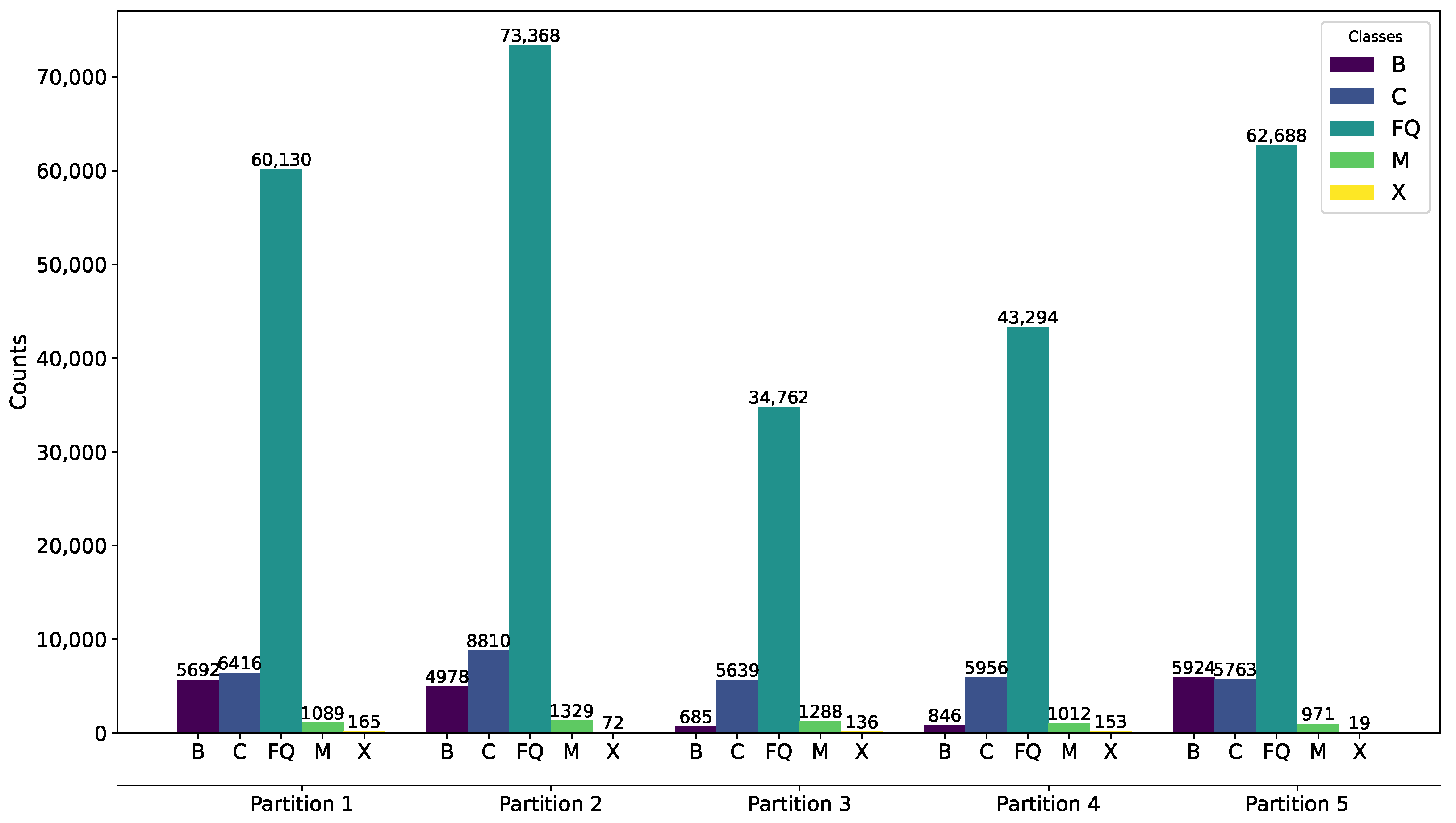
When the frequency of one class is significantly higher or lower than the others, the data are considered imbalanced [34]. The SWAN-SF dataset exhibits a high degree of imbalance, primarily due to the uneven frequency of flare classes. To address this and ensure balanced representation, the dataset is strategically divided into five partitions, each defined by specific time periods that contain a roughly equal number of significant flare events, such as M- and X-class flares. These partitions correspond to different phases of Solar Cycle 24, with the first partition covering the period from 1 May 2010 to 12 March 2012. The second extends from 2 March 2012 to 28 October 2013. The third spans from 17 October 2013 to 14 June 2014. The fourth is from 2 June 2014 to 18 March 2015, and the fifth and final partition ranges from 7 March 2015 to 16 August 2018. This structured partitioning aids in maintaining dataset balance, facilitating more effective training and testing of the prediction models. Figure 1 illustrates the distribution of flare classes across these partitions, highlighting the strategic data management employed.
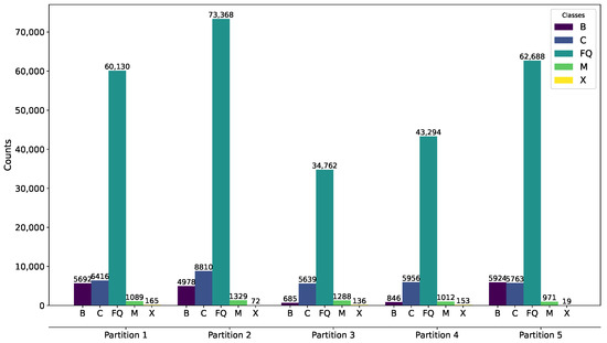
Figure 1.
SWAN-SF flare class distribution.
Data Pre-Processing
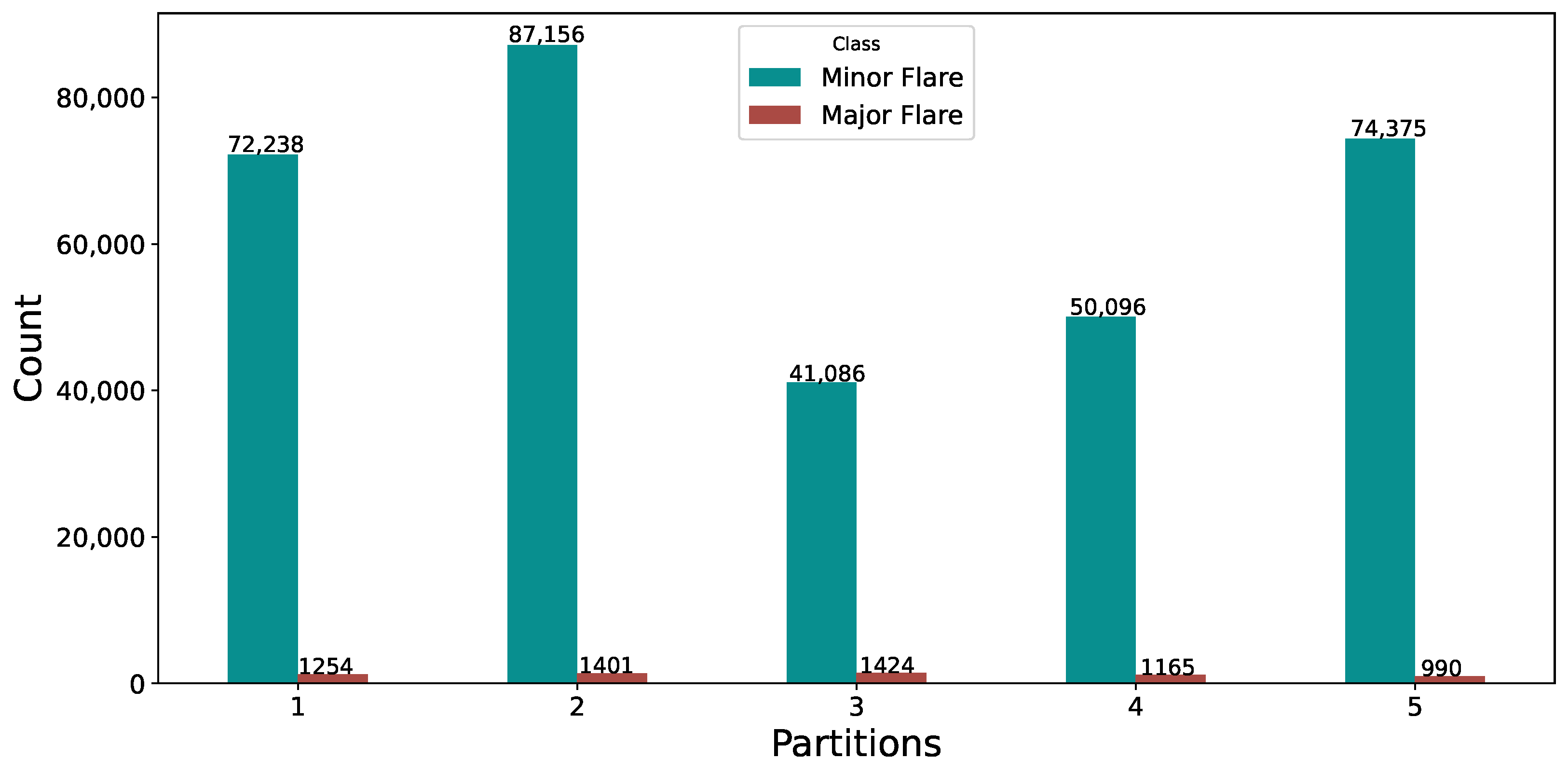
For this study, the SWAN-SF dataset has been restructured into a binary class format. Major flare classes that are significant enough to impact space weather, specifically M and X classes, are consolidated into a single category labeled as ‘1’, indicating the presence of active flare events. Concurrently, less intense B and C class flares, along with Flare Quiet (FQ) periods, are grouped under the label ‘0’, representing minor flare instances, as shown in Figure 2.

Figure 2.
SWAN-SF flare class distribution after binary conversion.
This conversion is necessary to address the significant class imbalance and improve model performance. As noted by He et al. [35], class imbalance poses a challenge in machine learning by making it difficult for the model to learn effectively from underrepresented classes. In the original multiclass setup, the disparity between the frequent B- and C-class flares and the rarer M- and X-class flares made it challenging for the model to accurately distinguish between them, potentially leading to biased predictions. By converting to binary classification, the model focuses on the fundamental distinction between major flare and minor flare events, simplifying the classification task and enabling more reliable and interpretable results [36]. In our refined approach, B and C class flares, as well as Flare Quiet (FQ) periods, are categorized as ‘Minor Flares’ events to prevent the misclassification of less intense flares as significant events. Only M- and X-class flares, known for their intensity and reliable detection, are classified as ‘Major Flare’ events. This methodical segregation helps maintain the integrity of our predictions by ensuring they are based on robust and accurately detected flare activities.
Data Imputation: The Fast Pearson Correlation-based K-nearest neighbors (FPCKNN) imputation method was employed to address any missing values in the dataset. FPCKNN is based on the K-nearest neighbors (KNNs) imputation, which fills in missing data by considering the values of the nearest neighbors [37]. This method ensures that the imputed values are consistent with the surrounding data points, preserving the integrity of the dataset for further analysis.
Normalization: The normalization of the dataset is performed using the Log, Square root, Box–Cox, Z-score, and MinMax (LSBZM) normalization method. This technique involves multiple steps: log transformation, square root transformation, Box–Cox transformation, z-score normalization, and min-max normalization. These steps are applied based on the skewness and standard deviation of each feature in the dataset [37]. The entire processed dataset is available at [38]. The comprehensive normalization process ensures that the data are appropriately scaled and transformed, which is crucial for improving the performance of the classifiers.
3. Methodology
The goal is to improve solar flare classification by utilizing feature selection methods and classifiers, integrating them into an ensemble approach, as shown in Figure 3. The methodology involves four key steps—baseline feature selection, classifier training and evaluation, and ensemble feature weight calculation—as outlined in Algorithm 1.
| Algorithm 1 Feature Weight Calculation |
|
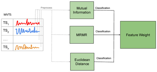
Figure 3.
Ensemble architecture.
3.1. Baseline Feature Selection Methods
- Mutual Information (MI): MI measures the mutual dependence between two variables, indicating how much information one variable contains about the other. For feature and target variable Y, MI is defined as follows:where is the joint probability distribution of and Y, and and are the marginal probability distributions.
- Minimum Redundancy Maximum Relevance (mRMR): mRMR aims to select features with high relevance with the target variable and low redundancy among themselves. For a feature subset S, mRMR is defined as follows:where is the relevance of feature to the target Y, and is the redundancy between features and .
- Euclidean Distance: This method selects features based on the Euclidean Distance between feature vectors in the feature space, aiming to maximize the separation between different classes. The Euclidean Distance between two points X and Y in an n-dimensional space is given by the following:
3.2. Classifier Training and Evaluation
The selected features are utilized to train and evaluate three classifiers: MINIROCKET, ROCKET, and Random Forest. Each was chosen for its distinct advantages in handling the challenges of solar flare classification, particularly in the context of large-scale, imbalanced datasets.
MINIROCKET and ROCKET: MINIROCKET and ROCKET are advanced time-series classifiers that leverage convolutional kernel transformations to capture and process complex temporal patterns in the data effectively. MINIROCKET, a streamlined variant of ROCKET, is designed for efficiency, allowing it to handle large datasets with minimal computational overhead while maintaining high accuracy. These classifiers have demonstrated superior performance compared to traditional neural networks, such as LSTM [39], particularly in solar flare prediction tasks where rapid processing and accuracy are critical [13]. The ability of these classifiers to operate without extensive pre-processing, such as normalization or balancing of class distributions, further enhances their suitability for this study.
Random Forest: Random Forest is an ensemble learning method that constructs multiple decision trees during training, aggregating their outputs to improve prediction accuracy and robustness. This method is particularly effective in handling high-dimensional data and modeling complex interactions between features. Random Forest’s resistance to overfitting, especially in imbalanced datasets, makes it a reliable choice for solar flare classification. Additionally, it provides valuable insights into feature importance, helping to identify which solar magnetic parameters are most predictive of flare events [14]. This interpretability, combined with its strong performance across various classification tasks, justifies its inclusion in the ensemble of classifiers used in this study.
3.3. Evaluation Metric
Selecting the appropriate evaluation metric is crucial in assessing classifier performance, mainly when dealing with highly imbalanced datasets. Traditional metrics such as accuracy often fail to provide a meaningful evaluation in these contexts because they tend to disproportionately reflect the performance on the majority class, leading to potentially misleading conclusions about a model’s effectiveness. In the case of solar flare classification, where flare events are rare compared to minor flare events, accuracy can overestimate a model’s performance by emphasizing its ability to correctly classify the dominant minor flare class while ignoring its shortcomings in identifying the minority flare class. This necessitates using more robust metrics that offer a balanced evaluation of both positive and negative predictions.
The True Skill Statistic (TSS) is particularly well-suited for such scenarios, as it integrates Sensitivity (true positive rate) and Specificity (true negative rate) into a single, coherent measure. TSS is calculated as follows:
where is the number of true positives, is the number of false negatives, is the number of false positives, and is the number of true negatives.
The primary strength of TSS lies in its independence from the base rate, ensuring that the metric remains consistent regardless of the class distribution within the dataset [40,41]. This property makes TSS a reliable choice for evaluating model performance in imbalanced datasets, such as those used in solar flare prediction, where the accurate identification of rare events is critical. In contrast, while valuable for understanding the performance on the positive class, metrics like Precision and Recall do not account for the correct classification of negative cases, potentially leading to an incomplete assessment of the model’s overall performance [35]. The F1-score, which balances Precision and Recall, similarly fails to consider the negative class, making it less suitable in highly imbalanced scenarios. The Heidke Skill Score (HSS), although comprehensive in considering the entire confusion matrix, is sensitive to the underlying class distribution, which can result in biased evaluations when the dataset is skewed [42]. Consequently, TSS is favored for its ability to provide a more accurate, stable, and interpretable assessment of classifier performance in environments where rare and common event detection is crucial.
3.4. Ensemble Feature Weight Calculation
The ensemble method aims to enhance the robustness of solar flare classification by integrating multiple feature selection techniques and classifiers. The feature weights are calculated using the following formula:
where is the final weight of feature f. is the median TSS score for the method-classifier combination across all subsets. is the median TSS score for feature f within the method-classifier combination across the subsets where feature f is present.
This method is designed to result in a more robust and generalizable model by balancing the contributions of diverse methods and classifiers. It achieves this by calculating the TSS for each method-classifier combination across various feature subsets, with the median TSS serving as the weight for each combination. This median captures consistent performance and reduces the influence of outliers. For individual features, the TSS is calculated specifically for subsets where the feature is present, and the median TSS of these subsets is taken as the feature score. By multiplying the feature score by the method-classifier weight, the final feature weight is derived, prioritizing features identified by more reliable combinations. This method is designed to result in a more robust and generalizable model by balancing the contributions of diverse methods and classifiers, potentially leading to improved performance on unseen data.The detailed algorithm for calculating the feature weights is as shown in Algorithm 1.
4. Experiments
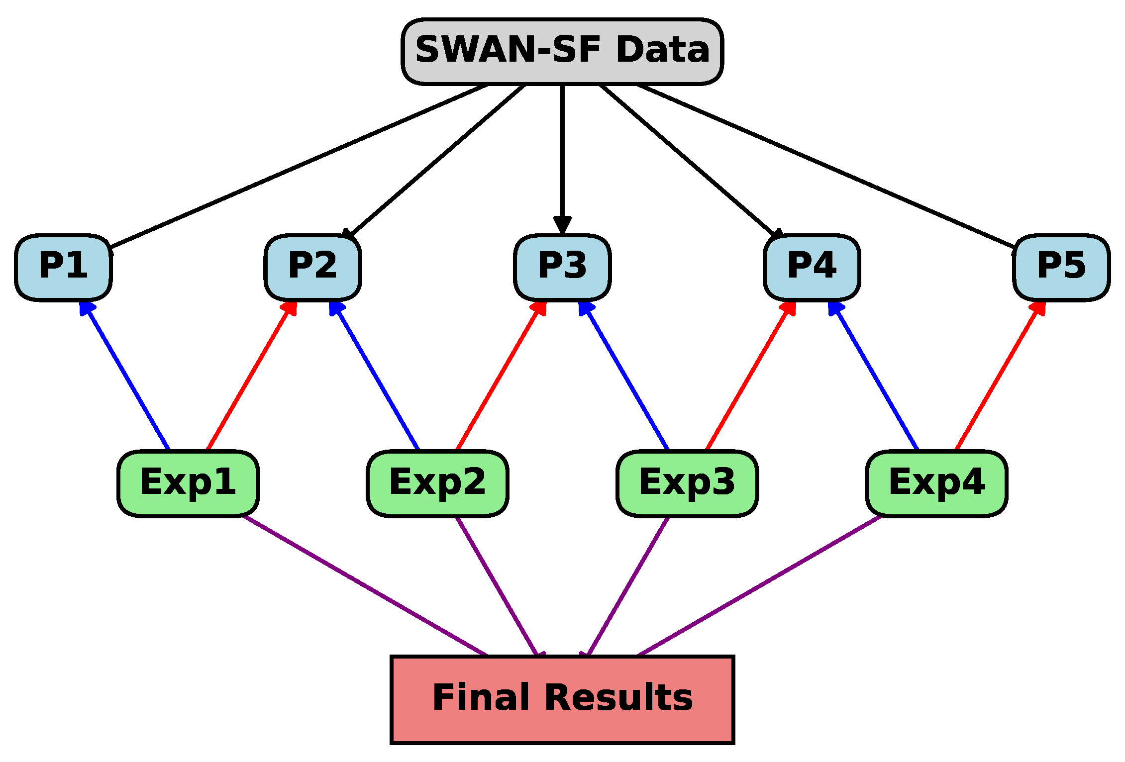
The SWAN-SF dataset is partitioned into five consecutive sections, with a systematic training and testing strategy. Initially, Partition 1 is used for training, while Partition 2 serves as the testing set. In the next iteration, Partition 2 becomes the training set, and Partition 3 is used for testing. This process continues sequentially, with Partition 3 used for training and Partition 4 for testing, followed by Partition 4 for training and Partition 5 for testing.
The rationale for this experimental setup is that using consecutive partitions maintains the natural order of the data, which is crucial in time-series analysis, as past events often influence future outcomes. Training on one partition and testing on the next ensures that the model learns to forecast future values based on the most relevant preceding information, closely replicating real-world scenarios where future data points succeed past ones.
Testing on the subsequent partition evaluates the model’s robustness to new, unseen conditions. This approach checks the model’s ability to adapt to changing situations it has not encountered during training, providing a substantial measure of its generalization to new data.
This method reflects the practical use of models in real-time applications. In many real-world scenarios, models are trained on historical data and are expected to make predictions on future data. By structuring experiments in this way, the model’s performance offers a realistic estimate of its effectiveness in operational environments.
To ensure stability and standardize the results, we conducted hold-out validation on each experiment five times. The outcomes of these validations were averaged to obtain a mean result. Subsequently, the results from all the experiments were combined based on the length of the subset for each classifier, as shown in Figure 4. This aggregation provided a comprehensive evaluation of the feature selection methods across different partitions, ensuring that the final results are robust and accurately reflect the model’s performance over the entire dataset.

Figure 4.
Experiment structure.
5. Results
The performance of the classifiers (MINIROCKET, ROCKET, and Random Forest) combined with different feature selection methods (Mutual Information, mRMR, Euclidean Distance, and Ensemble) was evaluated using the TSS metric. The mean TSS values were calculated for each feature selection method and classifier. It is important to note that the TSS values used to calculate the mean are not normally distributed.
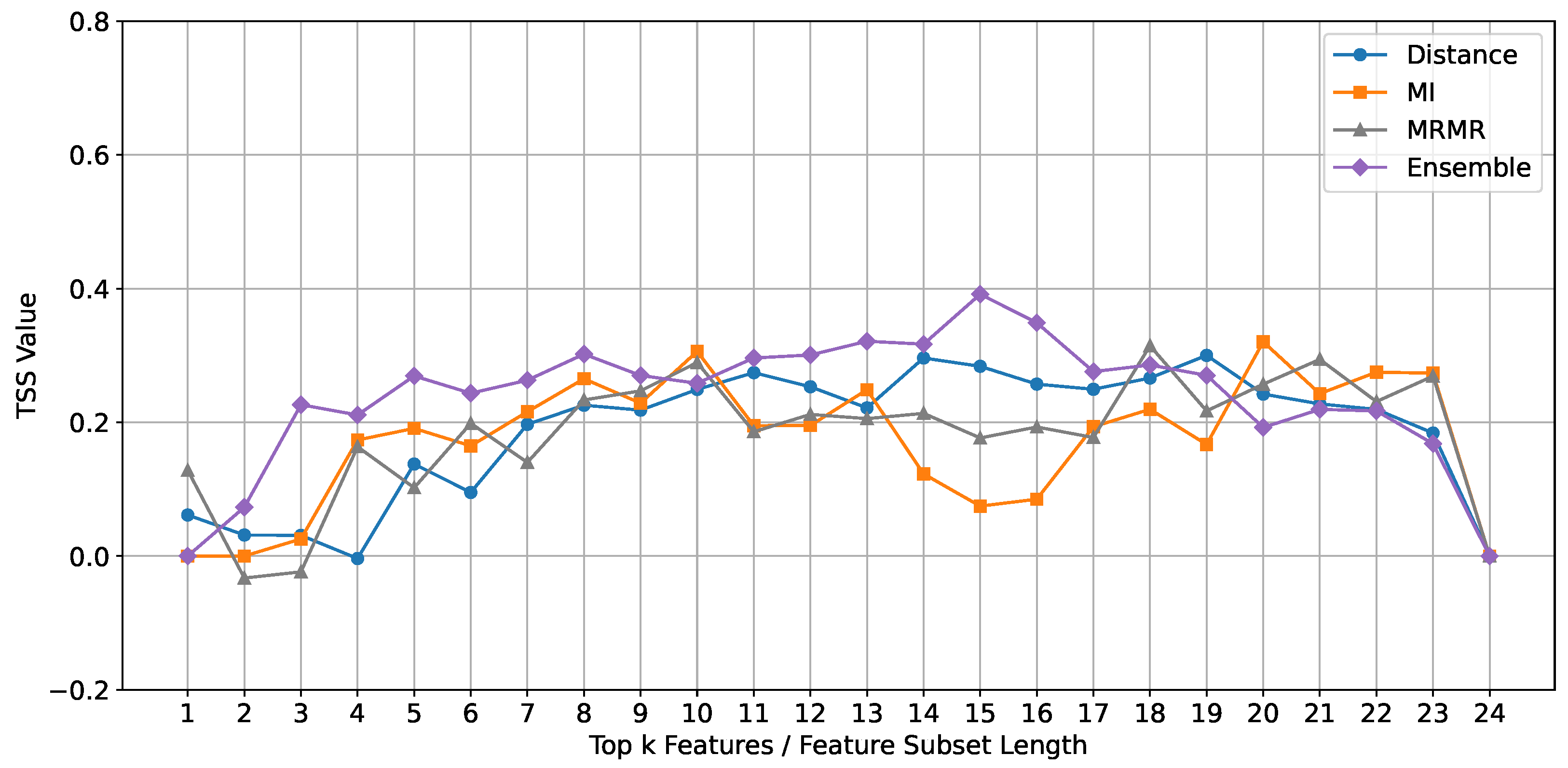
ROCKET: The performance of the ROCKET classifier, evaluated using the TSS metric, is depicted in Figure 5. The results indicate that the ensemble feature selection method consistently outperforms the individual methods (Mutual Information, mRMR, and Euclidean Distance) across different feature subset lengths.
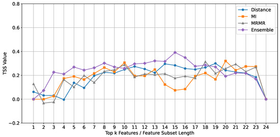
Figure 5.
Comparison of TSS mean values across different feature subset lengths for different feature selection methods using the Rocket classifier.
Upon closer examination, we observe that the ensemble method shows a notable improvement in TSS values for feature subset lengths ranging from 10 to 15. This suggests that the optimal subset range for the ROCKET classifier lies within 10 to 15 features. This range is significant because it balances complexity and simplicity, both too complex to cause overfitting and too simple to result in underfitting.
For the baseline methods, while there is a decline in the performance curves after ten features, we observe an interesting trend. After 19 features, there is an increase in the TSS values again. This indicates that while the performance initially drops due to potential noise and redundancy, including additional features beyond a certain point might capture some previously missed relevant information, improving classification performance.
However, the ensemble method clearly declines performance after 15 features. This highlights that including too many features beyond this point introduces unnecessary complexity and noise, which negatively impacts the classifier’s performance. Therefore, the feature subset length of 10 to 15 is optimal for achieving high classification accuracy with the ROCKET classifier using the ensemble method.
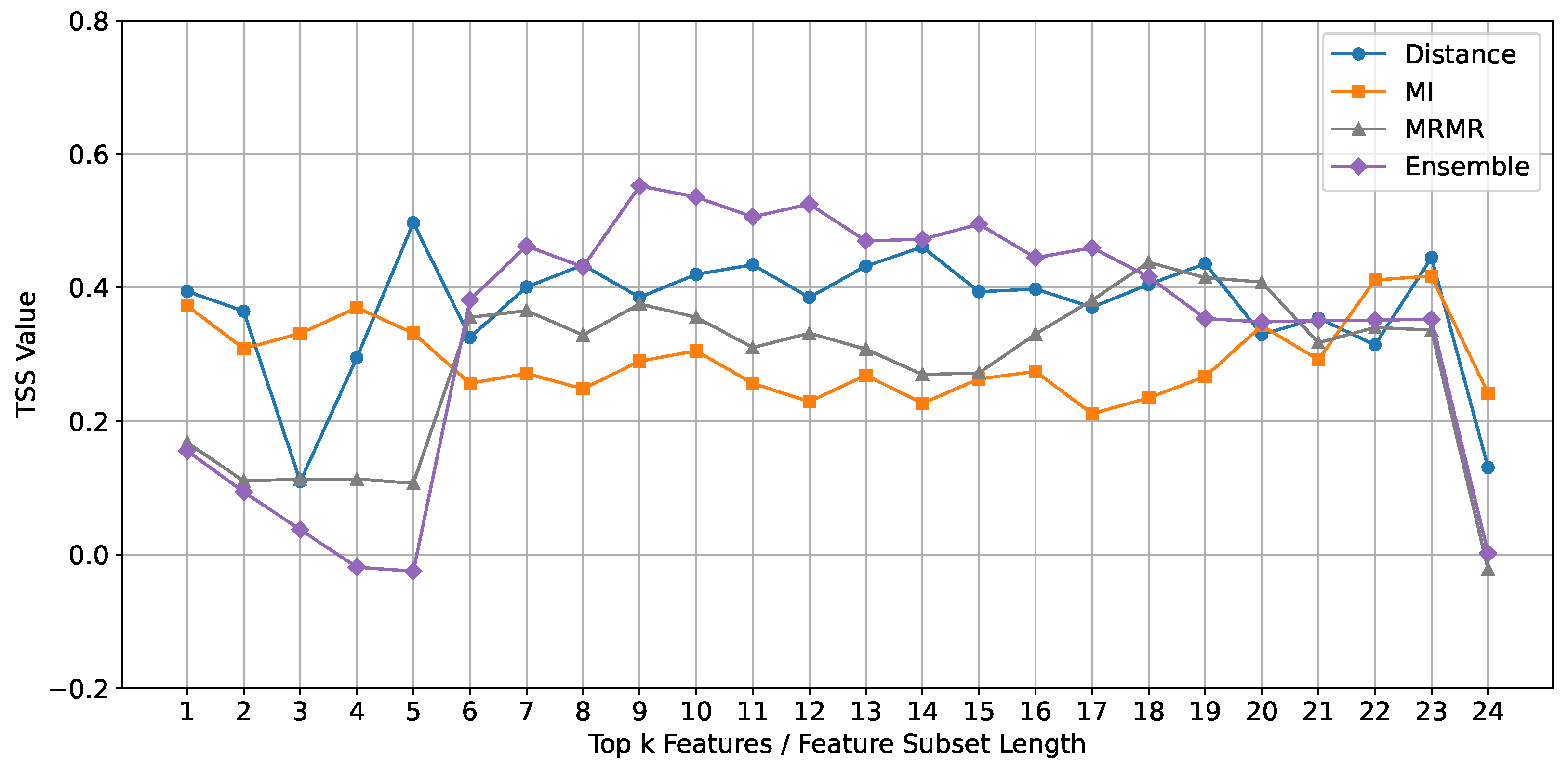
Random Forest Classifier: The performance of the Random Forest classifier, evaluated using the TSS metric, is depicted in Figure 6. The results indicate that the ensemble feature selection method consistently outperforms the individual methods (Mutual Information, mRMR, and Euclidean Distance) across different feature subset lengths.
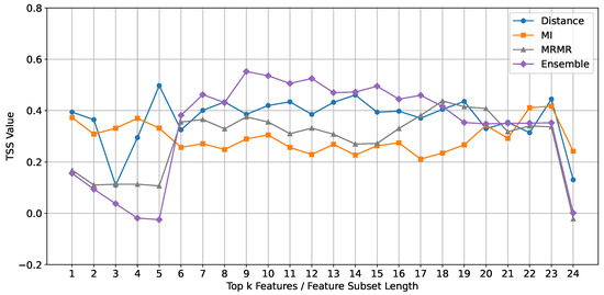
Figure 6.
Comparison of TSS mean values across different feature subset lengths for different feature selection methods using the Random Forest classifier.
Upon closer examination, we observe that the ensemble method shows a notable improvement in TSS values for feature subset lengths ranging from 9 to 15. This suggests that the optimal subset range for the Random Forest classifier lies within 9 to 15 features. This range is significant because it balances complexity and simplicity.
For the ensemble method, performance clearly declines after 15 features, indicating that including too many features beyond this point introduces unnecessary complexity and noise, which negatively impacts the classifier’s performance. In contrast, for the baseline methods (mRMR and Mutual Information), the performance curves increase after 15 features. This suggests that additional features may capture relevant information that is not apparent, leading to improved classification performance.
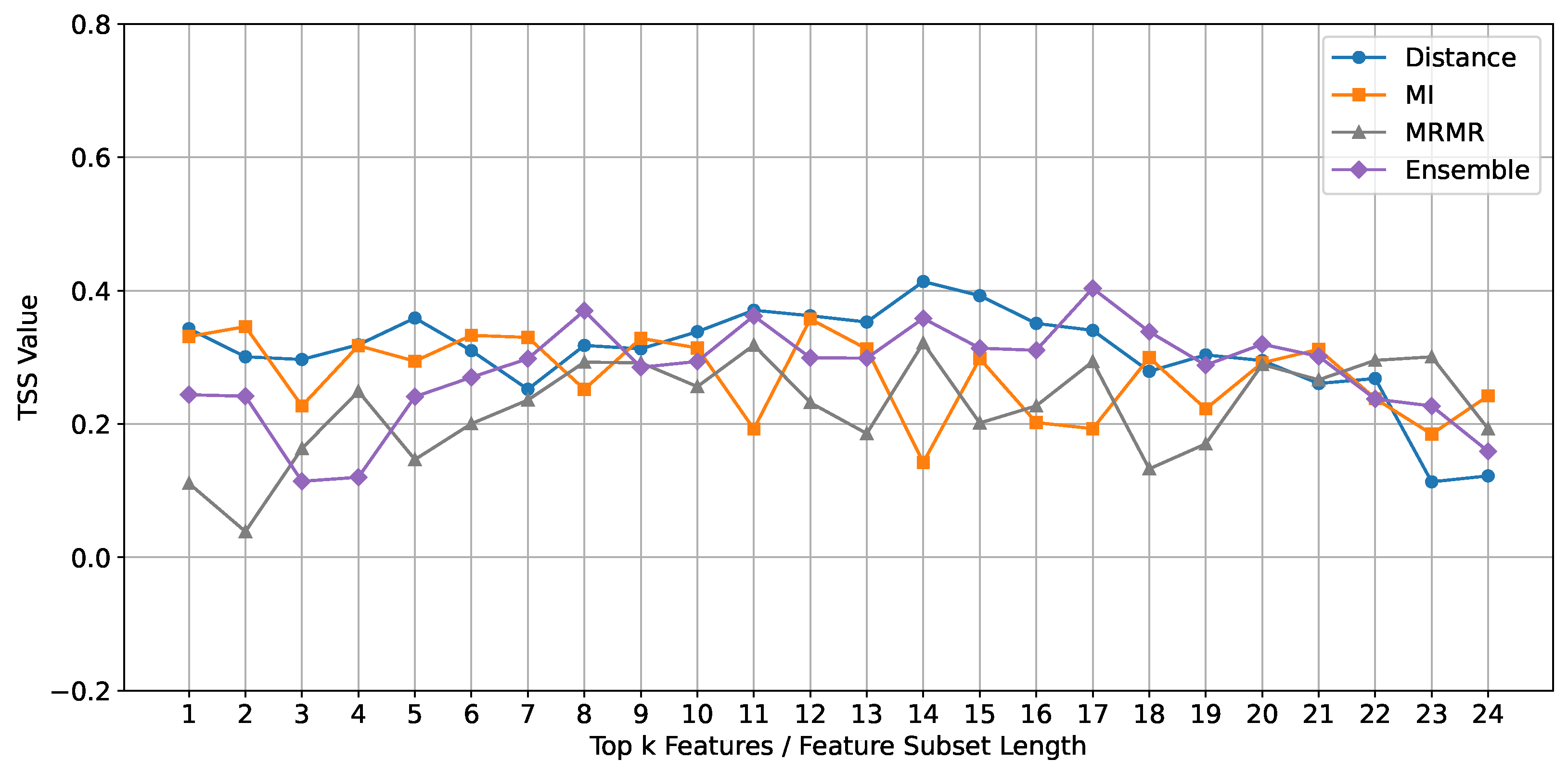
MINIROCKET Classifier: The performance of the MINIROCKET classifier, evaluated using the TSS metric, is depicted in Figure 7. Unlike the ROCKET and Random Forest classifiers, the ensemble feature selection method does not consistently outperform the individual methods (Mutual Information, mRMR, and Euclidean Distance) for MINIROCKET. Instead, the Euclidean Distance method shows better performance across feature subset lengths ranging from 10 to 15.
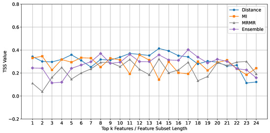
Figure 7.
Comparison of TSS mean values across different feature subset lengths for different feature selection methods using the MINIROCKET classifier.
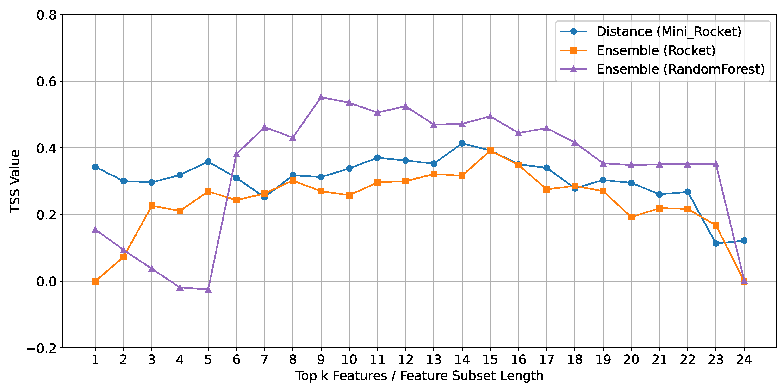
Despite the overall effectiveness of the ensemble method with ROCKET and Random Forest, MINIROCKET achieved a similar performance using the Euclidean Distance method, demonstrating its unique suitability for this classifier. The Euclidean Distance method calculates the straight-line distance between data points in a multi-dimensional space, effectively identifying and prioritizing the most relevant features for classification. When comparing the best results from each classifier in Figure 8, Random Forest produced the highest overall performance, followed by MINIROCKET, and then ROCKET. Notably, the Euclidean Distance method using MINIROCKET outperformed the ensemble method used with ROCKET, illustrating that even though MINIROCKET did not excel with the more complex ensemble method, it still delivered superior results, highlighting the potential advantages of a more straightforward feature selection strategy in specific scenarios.
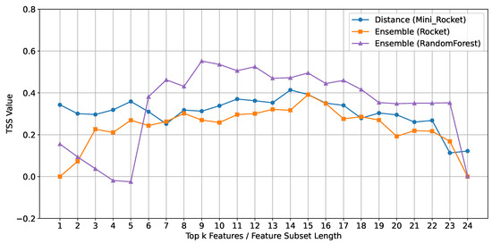
Figure 8.
Comparison of mean TSS values across feature subset lengths for best feature selection methods by classifier.
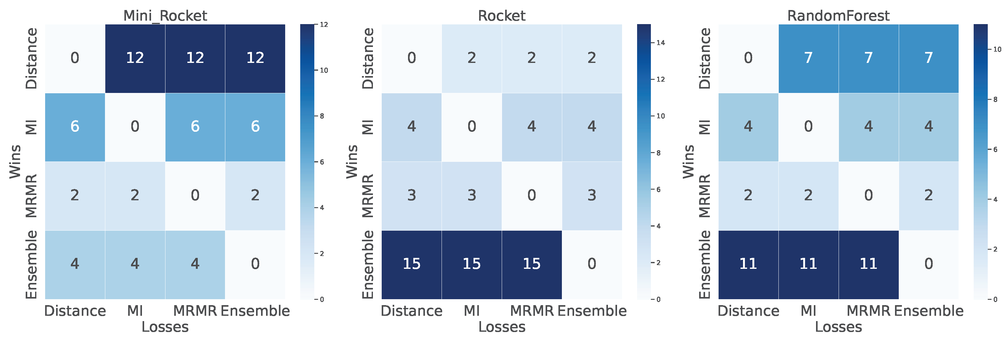
To provide a comprehensive comparison of the feature selection methods across different classifiers, a win–loss heat map was employed, as depicted in Figure 9. This heat map illustrates the number of times each feature selection method (Mutual Information, mRMR, Euclidean Distance, and Ensemble) outperformed the others across the three classifiers (MINIROCKET, ROCKET, and Random Forest). Each cell in the heat map represents the count of wins and losses for a specific feature selection method against another method for a given classifier, with darker shades indicating a higher count of wins.
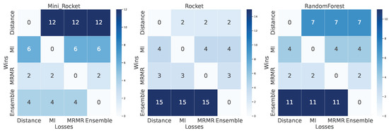
Figure 9.
Pairwise comparison of wins and losses among feature selection methods across different classifiers (MiniRocket, Rocket, Random Forest).
For the MINIROCKET classifier, the Euclidean Distance method showed the highest count of wins, suggesting its effectiveness in capturing relevant features for this classifier. In contrast, the ensemble method had relatively fewer wins for MINIROCKET, indicating it may not be as suitable for this specific classifier. For the ROCKET and Random Forest classifier, the ensemble method demonstrated the highest count of wins, showcasing its ability to enhance classification accuracy by effectively selecting relevant features.
As shown in Figure 9, the win–loss heat map highlights the relative performance consistency of each feature selection method across different classifiers. The ensemble method consistently showed a high count of wins across the ROCKET and Random Forest classifiers but less for MINIROCKET. The Euclidean Distance method demonstrated high variability, performing well for MINIROCKET but less consistently for the other classifiers. This comparative analysis underscores the strengths and weaknesses of each method, guiding future research in selecting appropriate feature selection techniques based on the classifier and dataset characteristics.
6. Discussion
The ensemble approach involves calculating feature weights based on TSS values obtained from classifiers. While this methodology theoretically enhances classifier performance, the practical outcomes vary. Empirically, ROCKET and Random Forest show improved performance with the ensemble-enhanced feature set. ROCKET’s architecture, characterized by random convolutional kernels, and Random Forest’s ensemble of decision trees effectively utilize diverse and comprehensive features. This allows for capturing a wide array of patterns and making more accurate splits, thereby enhancing classification accuracy and stability. Conversely, MINIROCKET, which employs a small, fixed set of convolutional kernels optimized for efficiency, encounters difficulties with the complexity introduced by the ensemble method. The fixed and deterministic nature of MINIROCKET’s kernels might limit its ability to adapt to the varied and enriched feature set, resulting in suboptimal performance. These findings indicate that the practical efficacy of the ensemble approach is significantly influenced by the classifiers’ intrinsic adaptability and architectural design.
The top 15 features selected through the ensemble method capture critical aspects of solar magnetic field dynamics. Helicity-related features, such as ABSNJZH (absolute value of the net current helicity), TOTUSJH (total unsigned current helicity), and MEANJZH (mean current helicity, Bz contribution), are crucial in identifying regions with significant magnetic twist and shear. According to Leka et al. [28], net current helicity is a significant indicator of the magnetic complexity and twist within active regions. High helicity values are associated with regions that have stored significant magnetic energy, making them more likely to produce solar flares. This relationship is critical for understanding the potential for flare activity, as regions with higher helicity are often sites of intense magnetic activity.
Magnetic free energy parameters, including TOTPOT (total photospheric magnetic free energy density) and MEANPOT (mean photospheric magnetic free energy), quantify the available magnetic energy in the photosphere. Schrijver et al. [32] states that higher values in these features correlate with an increased likelihood of energy release events, making them pivotal for reliable solar flare predictions. These features are essential for assessing flare potential because they measure the stored magnetic energy in the solar atmosphere. High magnetic free energy densities suggest that a significant amount of energy is available for release, thus increasing the probability of flare occurrence.
Magnetic current and flux parameters such as SAVNCPP (sum of the modulus of the net current per polarity), TOTUSJZ (total unsigned vertical current), and USFLUX (total unsigned flux) identify regions with intense magnetic activity and stress, essential precursors to flare initiation. The sum of flux near polarity inversion lines is particularly significant for identifying regions prone to magnetic reconnection, a fundamental process in flare genesis. These features help pinpoint areas of high magnetic stress and potential energy release. High values in these parameters indicate regions where the magnetic field is highly complex and dynamic, often leading to solar flares.
The Lorentz force components (TOTFX, TOTFY, TOTFZ) and the total magnitude of the Lorentz force (TOTBSQ), along with the sum of the z-component of normalized Lorentz force (EPSZ), provide a comprehensive view of the forces acting within the magnetic field. Fisher et al. [29] emphasize that these forces are critical in destabilizing the magnetic configuration, facilitating the release of stored magnetic energy, which indicates flare triggers. Understanding the distribution and magnitude of the Lorentz force is crucial for identifying regions where the magnetic field is likely to become unstable and release energy in the form of flares.
Magnetic field topology parameters such as MEANALP (mean characteristic twist parameter, ) and MEANGAM (mean angle of the field from radial) describe the configuration and orientation of the magnetic field. High values of these parameters reflect significant magnetic twists and inclinations, essential for understanding the buildup of magnetic energy and the potential for reconnection events. The fraction of area with shear more significant than 45 degrees (SHRGT45) identifies regions with significant shear, often associated with magnetic instability and flare activity. Wang et al. [31] note that high shear values indicate areas where the magnetic field lines are highly stressed and likely to reconnect.
7. Conclusions
In this study, we developed an ensemble approach that integrates feature selection methods and classifiers to improve solar flare classification. We employed feature selection techniques, including Mutual Information (MI), Minimum Redundancy Maximum Relevance (mRMR), and Euclidean Distance, to identify the most relevant magnetic field parameters from multivariate time-series data. These methods helped us reduce the dimensionality of the data and focus on the features most strongly correlated with solar flare activity.
The ensemble approach was then applied, combining the outputs of these feature selection methods with multiple classifiers ROCKET, MINIROCKET, and Random Forest. By integrating the strengths of both the feature selection methods and the classifiers, we were able to create a robust framework that leverages the unique capabilities of each component. This approach allowed us to capture complex patterns in the data and improve the overall predictive performance of the models.
Our results showed that this ensemble method significantly enhanced the accuracy of solar flare classification. The ROCKET and Random Forest classifiers, in particular, demonstrated substantial improvements in True Skill Statistic (TSS) values, reflecting their ability to utilize the optimized feature sets effectively. MINIROCKET also benefited from the ensemble approach, although its performance was slightly less notable due to its fixed kernel structure.
In conclusion, this research has shown that an ensemble approach that incorporates both feature selection methods and classifiers can significantly improve solar flare classification accuracy. The methodologies developed in this study provide a solid foundation for future research in space weather forecasting, offering a versatile and effective strategy for enhancing predictive models in the face of complex and imbalanced datasets.
Author Contributions
Conceptualization, Y.V., P.H. and S.F.B.; methodology, Y.V. and S.F.B.; software, Y.V.; validation, P.H. and S.F.B.; formal analysis, Y.V.; investigation, Y.V.; resources, S.F.B. and S.M.H.; data curation, Y.V.; writing—original draft preparation, Y.V.; writing—review and editing, P.H. and Y.V.; visualization, Y.V.; supervision, S.F.B. and S.M.H.; project administration, S.F.B.; funding acquisition, S.F.B. All authors have read and agreed to the published version of the manuscript.
Funding
This project has been supported in part by funding from CISE and GEO Directorates under NSF awards #2204363, #2240022, #2301397, and #2305781.
Data Availability Statement
Data derived from public domain resources. See related links and references cited in the main text of the paper.
Conflicts of Interest
The authors declare no conflicts of interest.
References
- Benz, A.O. Flare Observations. Living Rev. Sol. Phys. 2017, 14, 1–59. [Google Scholar] [CrossRef]
- Angryk, R.A.; Martens, P.C.; Aydin, B.; Kempton, D.; Mahajan, S.S.; Basodi, S.; Ahmadzadeh, A.; Cai, X.; Filali Boubrahimi, S.; Hamdi, S.M.; et al. Multivariate Time Series Dataset for Space Weather Data Analytics. Sci. Data 2020, 7, 227. [Google Scholar] [CrossRef] [PubMed]
- Howard, T. Coronal Mass Ejections: An Introduction; Springer Science & Business Media: New York, NY, USA, 2011; Volume 376. [Google Scholar] [CrossRef]
- National Research Council. Severe Space Weather Events: Understanding Societal and Economic Impacts: A Workshop Report; The National Academies Press: Washington, DC, USA, 2009. [Google Scholar] [CrossRef]
- Hosseinzadeh, P.; Boubrahimi, S.F.; Hamdi, S.M. Improving solar energetic particle event prediction through multivariate time series data augmentation. Astrophys. J. Suppl. Ser. 2024, 270, 31. [Google Scholar] [CrossRef]
- Hosseinzadeh, P.; Filali Boubrahimi, S.; Hamdi, S.M. Toward enhanced prediction of high-impact solar energetic particle events using multimodal time series data fusion models. Space Weather 2024, 22, e2024SW003982. [Google Scholar] [CrossRef]
- Hapgood, M.A. Towards a Scientific Understanding of the Risk from Extreme Space Weather. Adv. Space Res. 2011, 47, 2059–2072. [Google Scholar] [CrossRef]
- Carrington, R.C. Description of a Singular Appearance Seen in the Sun on September 1, 1859. Mon. Not. R. Astron. Soc. 1859, 20, 13–15. [Google Scholar] [CrossRef]
- Bobra, M.G.; Couvidat, S. Solar Flare Prediction Using SDO/HMI Vector Magnetic Field Data with a Machine-Learning Algorithm. Astrophys. J. 2015, 798, 135. [Google Scholar] [CrossRef]
- Ircio, J.; Lojo, A.; Mori, U.; Lozano, J.A. Mutual Information-Based Feature Subset Selection in Multivariate Time Series Classification. Pattern Recognit. 2020, 108, 107525. [Google Scholar] [CrossRef]
- He, C.; Huo, X.; Zhu, C.; Chen, S. Minimum Redundancy Maximum Relevancy-Based Multiview Generation for Time Series Sensor Data Classification and Its Application. IEEE Sens. J. 2024, 24, 12830–12839. [Google Scholar] [CrossRef]
- Patel, S.P.; Upadhyay, S.H. Euclidean Distance Based Feature Ranking and Subset Selection for Bearing Fault Diagnosis. Expert Syst. Appl. 2020, 154, 113400. [Google Scholar] [CrossRef]
- Saini, K.; Alshammari, K.; Hamdi, S.M.; Filali Boubrahimi, S. Classification of Major Solar Flares from Extremely Imbalanced Multivariate Time Series Data Using Minimally Random Convolutional Kernel Transform. Universe 2024, 10, 234. [Google Scholar] [CrossRef]
- Ma, R.; Boubrahimi, S.F.; Hamdi, S.M.; Angryk, R.A. Solar Flare Prediction Using Multivariate Time Series Decision Trees. In Proceedings of the 2017 IEEE International Conference on Big Data (Big Data), Boston, MA, USA, 11–14 December 2017; pp. 2569–2578. [Google Scholar] [CrossRef]
- Filali Boubrahimi, S.; Neema, A.; Nassar, A.; Hosseinzadeh, P.; Hamdi, S.M. Spatiotemporal Data Augmentation of MODIS-Landsat Water Bodies Using Adversarial Networks. Water Resour. Res. 2024, 60, e2023WR036342. [Google Scholar] [CrossRef]
- EskandariNasab, M.; Raeisi, Z.; Lashaki, R.A.; Najafi, H. A GRU–CNN model for auditory attention detection using microstate and recurrence quantification analysis. Sci. Rep. 2024, 14, 8861. [Google Scholar] [CrossRef] [PubMed]
- Yang, K.; Yoon, H.; Shahabi, C. A Supervised Feature Subset Selection Technique for Multivariate Time Series. In Proceedings of the Workshop on Feature Selection for Data Mining: Interfacing Machine Learning with Statistics, Newport Beach, CA, USA, 21–23 April 2005; pp. 92–101. [Google Scholar]
- Yin, L.; Ge, Y.; Xiao, K.; Wang, X.; Quan, X. Feature Selection for High-Dimensional Imbalanced Data. Neurocomputing 2013, 105, 3–11. [Google Scholar] [CrossRef]
- Muzaheed, A.A.M.; Hamdi, S.M.; Boubrahimi, S.F. Sequence Model-Based End-to-End Solar Flare Classification from Multivariate Time Series Data. In Proceedings of the 2021 20th IEEE International Conference on Machine Learning and Applications (ICMLA), Pasadena, CA, USA, 13–16 December 2021; pp. 435–440. [Google Scholar] [CrossRef]
- Hoeksema, J.T.; Liu, Y.; Hayashi, K.; Sun, X.; Schou, J.; Couvidat, S.; Norton, A.; Bobra, M.; Centeno, R.; Leka, K.D.; et al. The Helioseismic and Magnetic Imager (HMI) Vector Magnetic Field Pipeline: Overview and Performance. Sol. Phys. 2014, 289, 3483–3530. [Google Scholar] [CrossRef]
- Angryk, R.; Martens, P.; Aydin, B.; Kempton, D.; Mahajan, S.; Basodi, S.; Ahmadzadeh, A.; Cai, X.; Filali Boubrahimi, S.; Hamdi, S.M.; et al. SWAN-SF. Harvard Dataverse, 2020; V1. [Google Scholar] [CrossRef]
- Cui, Y.; Li, R.; Zhang, L.; He, Y.; Wang, H. Correlation Between Solar Flare Productivity and Photospheric Magnetic Field Properties: 1. Maximum Horizontal Gradient, Length of Neutral Line, Number of Singular Points. Sol. Phys. 2006, 237, 45–59. [Google Scholar] [CrossRef]
- Cui, Y.; Li, R.; Wang, H.; He, H. Correlation Between Solar Flare Productivity and Photospheric Magnetic Field Properties II. Magnetic Gradient and Magnetic Shear. Sol. Phys. 2007, 242, 1–8. [Google Scholar] [CrossRef]
- Georgoulis, M.K. On Our Ability to Predict Major Solar Flares. In The Sun: New Challenges: Proceedings of Symposium 3 of JENAM 2011; Springer: Berlin/Heidelberg, Germany, 2012. [Google Scholar] [CrossRef]
- Ahmed, O.W.; Qahwaji, R.; Colak, T.; Higgins, P.A.; Gallagher, P.T.; Bloomfield, D.S. Solar Flare Prediction Using Advanced Feature Extraction, Machine Learning, and Feature Selection. Sol. Phys. 2013, 283, 157–175. [Google Scholar] [CrossRef]
- Barnes, G.; Leka, K.D.; Schrijver, C.J.; Colak, T.; Qahwaji, R.; Ashamari, O.W.; Yuan, Y.; Zhang, J.; McAteer, R.T.J.; Bloomfield, D.S.; et al. A Comparison of Flare Forecasting Methods. I. Results from the “All-Clear” Workshop. Astrophys. J. 2016, 829, 89. [Google Scholar] [CrossRef]
- Su, Y.; Gan, W.Q.; Li, Y.P. A Statistical Study of RHESSI Flares. Sol. Phys. 2006, 238, 61–72. [Google Scholar] [CrossRef]
- Leka, K.; Barnes, G. Photospheric Magnetic Field Properties of Flaring Versus Flare-Quiet Active Regions. II. Discriminant Analysis. Astrophys. J. 2003, 595, 1296. [Google Scholar] [CrossRef]
- Fisher, G.H.; Bercik, D.J.; Welsch, B.T.; Hudson, H.S. Global Forces in Eruptive Solar Flares: The Lorentz Force Acting on the Solar Atmosphere and the Solar Interior. Sol. Phys. 2012, 277, 59–76. [Google Scholar] [CrossRef]
- Leka, K.; Skumanich, A. On the Value of ‘αAR’ from Vector Magnetograph Data. Sol. Phys. 1999, 188, 3–19. [Google Scholar] [CrossRef]
- Wang, J.; Shi, Z.; Wang, H.; Lue, Y. Flares and the Magnetic Nonpotentiality. Astrophys. J. 1996, 456, 861. [Google Scholar] [CrossRef]
- Schrijver, C.J. A characteristic magnetic field pattern associated with all major solar flares and its use in flare forecasting. Astrophys. J. 2007, 655, L117. [Google Scholar] [CrossRef]
- Ahmadzadeh, A.; Aydin, B.; Georgoulis, M.K.; Kempton, D.J.; Mahajan, S.S.; Angryk, R.A. How to train your flare prediction model: Revisiting robust sampling of rare events. Astrophys. J. Suppl. Ser. 2021, 254, 23. [Google Scholar] [CrossRef]
- Kubat, M.; Matwin, S. Addressing the Curse of Imbalanced Training Sets: One-Sided Selection. In Proceedings of the International Conference on Machine Learning, San Francisco, CA, USA, 8–12 July 1997; Volume 97, pp. 1–10. [Google Scholar]
- He, H.; Garcia, E.A. Learning from Imbalanced Data. IEEE Trans. Knowl. Data Eng. 2009, 21, 1263–1284. [Google Scholar] [CrossRef]
- Weiss, G.M. Mining with rarity: A unifying framework. ACM Sigkdd Explor. Newsl. 2004, 6, 7–19. [Google Scholar] [CrossRef]
- EskandariNasab, M.; Hamdi, S.M.; Filali Boubrahimi, S. SWAN-SF Data Preprocessing and Sampling Notebooks (v1.0.0). Zenodo 2024. [Google Scholar] [CrossRef]
- EskandariNasab, M.; Hamdi, S.M.; Filali Boubrahimi, S. Cleaned SWANSF Dataset (v1.0.0). Zenodo 2024. [Google Scholar] [CrossRef]
- Alshammari, K.; Hamdi, S.M.; Boubrahimi, S.F. Feature Selection from Multivariate Time Series Data: A Case Study of Solar Flare Prediction. In Proceedings of the 2022 IEEE International Conference on Big Data (Big Data), Osaka, Japan, 17–20 December 2022; pp. 4796–4801. [Google Scholar] [CrossRef]
- Bloomfield, D.S.; Higgins, P.A.; McAteer, R.T.J.; Gallagher, P.T. Toward Reliable Benchmarking of Solar Flare Forecasting Methods. Astrophys. J. Lett. 2012, 747, L41. [Google Scholar] [CrossRef]
- Woodcock, F. The Evaluation of Yes/No Forecasts for Scientific and Administrative Purposes. Mon. Weather Rev. 1976, 104, 1209–1214. [Google Scholar] [CrossRef]
- Ferri, C.; Hernández-Orallo, J.; Modroiu, R. An Experimental Comparison of Performance Measures for Classification. Pattern Recognit. Lett. 2009, 30, 27–38. [Google Scholar] [CrossRef]
Disclaimer/Publisher’s Note: The statements, opinions and data contained in all publications are solely those of the individual author(s) and contributor(s) and not of MDPI and/or the editor(s). MDPI and/or the editor(s) disclaim responsibility for any injury to people or property resulting from any ideas, methods, instructions or products referred to in the content. |
© 2024 by the authors. Licensee MDPI, Basel, Switzerland. This article is an open access article distributed under the terms and conditions of the Creative Commons Attribution (CC BY) license (https://creativecommons.org/licenses/by/4.0/).

