Article

Insect Diversity in the Coastal Pinewood and Marsh at Schinias, Marathon, Greece: Impact of Management Decisions on a Degraded Biotope

1
Laboratory of Entomology, Hellenic Agricultural Organization—“Demeter”, Institute for Mediterranean Forest Ecosystem Research, Terma Alkmanos, 11528 Athens, Greece
2
Laboratory of Forest Management and Economics, Hellenic Agricultural Organization—“Demeter”, Institute for Mediterranean Forest Ecosystem Research, Terma Alkmanos, 11528 Athens, Greece
3
Laboratory of Forest Ecology, Hellenic Agricultural Organization—“Demeter”, Institute for Mediterranean Forest Ecosystem Research, Terma Alkmanos, 11528 Athens, Greece
4
Hellenic Agricultural Organization—“Demeter”, Forest Research Institute, 57006 Vassilika, Thessaloniki, Greece
5
Water and Management Research Centre, Faculty of Engineering, University of Bristol, Bristol BS8 1TR, UK
*
Author to whom correspondence should be addressed.
Forests 2023, 14(2), 392; https://doi.org/10.3390/f14020392
Submission received: 16 December 2022 / Revised: 5 February 2023 / Accepted: 13 February 2023 / Published: 15 February 2023
(This article belongs to the Special Issue Management and Restoration of Post-disturbance Forests)

Abstract

:
The insects trapped in 63 plots positioned in a mixed pinewood and a marsh in Schinias, Marathon, Greece is studied relative to the anthropogenic disturbance. The last anthropogenic impact was recently intensified because of the Olympic Games in the area. One hundred and forty insect species were found that had abundances greater than two individuals in each sampling session in all plots. Seven insect community types were found using cluster analysis. The types, which corresponded to recognized habitats, re-emerged in a non-metric multidimensional scaling ordination. It was also found that insects tended to dwell in different plots, even in the same habitat. The invading P. halepensis Mill., which replaces P. pinea L., changed the entomofauna. The seven habitats had different numbers of bioindicators out of 74 insect species, not in general correlated with human impact. Three components of insect diversity were measured, and the temporal species turnover was consistently higher than the spatial one. In this sense, pine habitats were rated first in terms of overall insect diversity. In terms of biodiversity, the impact on the various biotopes was assessed utilizing the diversity–equitability index V, which indicated that the two P. halepensis-dominated habitats have negative V values together with the habitat dominated by Tamarix hampeana Nied. The conservation of P. pinea and the marsh habitats is recommended for conserving local entomofauna and stopping the progression of P. halepensis. The optimization of management strategies to meet the management goals of all elements of this degraded ecosystem seems to be crucial.

1. Introduction

Coastal sand dunes are among the most widespread habitats worldwide. Although sand dunes are among the first studied ecosystems (as early as 1835, according to Martinez and Psuty [1]), they are poorly known. This contrasts with their considerable socioeconomic value [2] and the fact that they are biotopes with highly evolved and adapted specialist species capable of occupying very fragile ecosystems of oscillating environmental variables, e.g., [3].
Their ability to respond to human-induced disturbance and climate changes and their proximity to human settlements make them good systems for the study of plant and insect communities [4,5,6,7,8,9,10], as well as individual species [11,12,13,14,15,16]. They are also used in the implementation of nature conservation measures [17]. The degradation of dune slacks continues apace, leading to the reduction in the area of coastal dune grasslands, together with a severe change to their geomorphology [5,12]. This is due to human draining projects that lower the water table and change the water availability to all successional dune stages. In addition, sand dunes and all successional stages show changes caused by human impact irrespective of the degree of resilience or sensitivity [4]. In Attica, Greece, the densely forested Holocene landscape with many coastal salt marshes and sandy plains [17] has over time degraded or been converted to agricultural land. This resulted from a series of occupations of the country by foreign forces and was followed by a final population increase and the associated construction works, of which salt marshes and littoral ecosystems were the first casualties [18]. The Marathon plain and Schinias escaped tourism and residential/holiday developments before the 1960s because of the presence of mosquitos. Since then, extensive control of the mosquito population by insecticide spraying led to intensified agricultural activities (authors’ observation).
The Schinias area is made up of biotopes that belong to endangered ecosystems of the Mediterranean [18]. Most of these coastal biotopes have already been destroyed (more than 90%—a fact that results in the area needing immediate conservation). For that reason, it has been included in the list of National Parks of Greece (in 2002), in the CORINE biotopes, and in the network of the Natura 2000 biotopes [19]. Unfortunately, the increased tourism value associated with the battlefield (590 BC) led to the selection of the area for the construction of the canoeing and rowing center for the 2004 Olympics. This accelerated the degradation of local ecosystems.
Conservation of insects can only be achieved through indirect measures that protect the biotopes where the species live [6,18,20,21]. The selection of the species and sites to be protected should be based on the current evaluation of the quantity and quality of biodiversity [22,23]. This information is generally lacking for many insects in Greece. This current work establishes the background for an objective risk assessment of the endangered species further to indirect conservation strategies [22]. For this, the biotic communities must be described, and the characteristic insect species that indicate the properties of each community type must be listed. This is achieved by finding the major community types of the studied area and the indicator species for each of these. Biotic communities should emerge from a set of plots. Description of these types is usually done by measuring the nestedness within this set of plots and the occurrence patterns of indicator species [24]. Biodiversity, as a property of communities, should be partitioned into spatial and temporal components [25]. The biodiversity of each plot, and the specificity of insect species within each habitat, give a good description of the insect communities [26].
The purpose of this paper is to find the types and properties of local insect communities and the necessary ecological regime leading to the development of efficient conservation strategies. The geomorphological history of Schinias is well-documented [27], together with the flora, entomofauna, and vegetation [18,28,29]. For this, Schinias is an ideal case for the analysis of human impacts on insect communities. In this research, the following aims were established: (a) to identify insect communities and the coherence with the classification of plots based on plant species, (b) to analyze the affinities of the insect communities and explore the effect of human impact on them and their response, (c) to identify the indicator insect species of the delimited biotic communities, and (d) to assess the functional role of the indicator species and their relationship with the anthropogenic impact type and amount in each habitat.

2. Materials and Methods
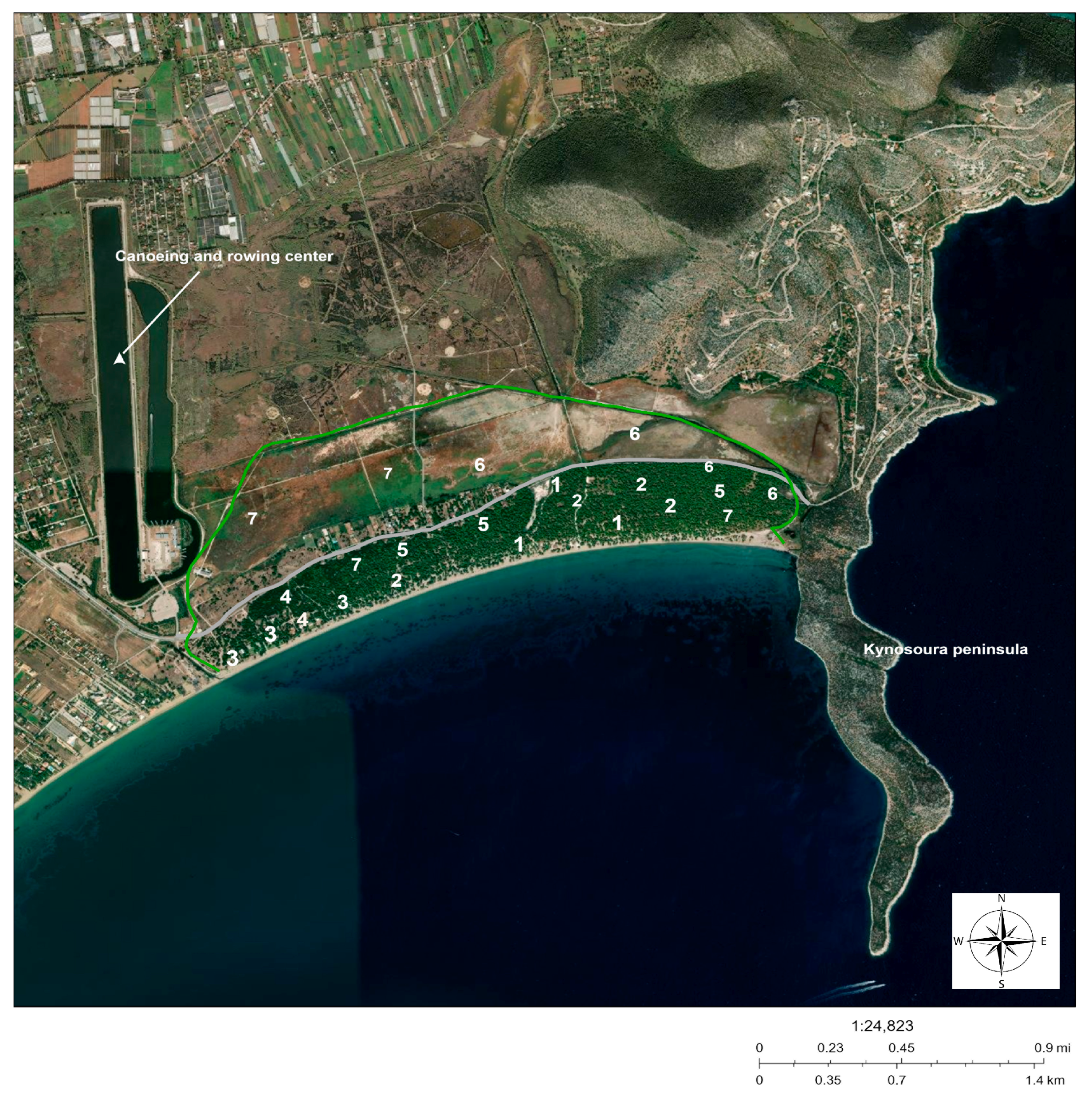
2.1. Study Area

Schinias is in the coastal area of Marathon village (E 24° 3′, N 38° 8′). The studied site includes dunes, coastal pinewood, and all successional stages between them, together with inland salt marsh (Figure 1). For the dune system, the terminology follows that of Knott and Warren [30]. The name of the area is derived from the dominant shrub Pistacia lentiscus (= Pa. lentiscus), Anacardiaceae; Greek name is schinon (pl. schina, adj. schinias). In the past, Pa. lentiscus formed dense thickets. The site is located in the northeastern part of the Attica Peninsula. Schinias is a typical east-Mediterranean area with high plant [18,31], insect [28,29], fish [32], and bird diversity [33]. Schinias is a biotope of ecological significance, despite its proximity to Athens, and is included in the biotopes of the NATURA network (code: GR3000003 in [19]). The biotope is characterized by a high diversity of habitat and vegetation types with 22 habitat types of European importance (Appendix A of Directive 92/43/EEC “on the conservation of natural habitats and of wild fauna and flora”, Table 1, (Figure A2). The area of Schinias presents a great variety of vegetation, which reflects the various soil and water conditions that prevail at this site. At the same time, however, it presents a strong picture of degradation and decline, which is associated with reckless human activity. There are four vegetation units: (1) the vegetation of sandy beaches, (2) the vegetation of wetlands, (3) the shrubs and the P. pinea forest, and (4) the P. halepensis forest. The ecological and cultural importance of the area is due to the Marathon battle in 490 BC (Pausanias 160 BC). This attracts a great number of visitors, which has recently further increased following the construction of the ‘canoeing and rowing center’ for the 2004 Olympic Games and all the construction related to the visitors.
Two springs, named Makaria and Drakonera, reduce the salinity of the marsh, while seawater increases it. Several small streams drain the marsh in springtime. In May, the entire marsh is dry, except for some small pools in the northern part of the marsh. The drainage ditch in the eastern part at the base of the Kynosoura Peninsula (Figure 1) creates ideal spawning grounds for many fishes and attracts many birds, while it sustains a multitude of plant associations [28,33,34].

2.2. Insect and Vegetation Sampling

Insects were sampled in 63 square plots, each one having sides of 5 m, randomly positioned with the aid of a random generator. Points that fell on unsuitable spots, such as houses, roads, and sea, or were closer than 50 m to other points, were discarded (Figure 1). Each plot had one side parallel to the shoreline. In the middle of each plot and at the four corners, pitfall traps were used to collect the ground fauna (= five per plot). Pitfall traps functioned all year round and were emptied and serviced once a week. The pots had a diameter of 12 cm and were filled with ethylene glycol: water 1:1 solution 3 cm deep. The lower vegetation layers were swept fortnightly for up to 5 min per plot, with an insect net having a diameter of 22 cm and a depth of 50 cm. Up to 4 window traps and 2 eclector traps [35] were set in each plot, where there was a pine-tree. This tree was used to sample bark beetles and dead wood dwelling (saproxylic) insects (bioform Dr. J. Schmidl e.k., Germany). Twice a year in April–May and September–October, a Malaise flight interception trap was set for 6 h in each plot (between 1000–1800 h) to collect all passing flying insects. Eight Malaise traps (7 traditional 6 m traps with two collecting jars and one Townes style) were used to sample each plot on one day. All plots were sampled within one week. A flight interception window trap was used fixed on tree trunks. The glass window was a 30 cm × 40 cm quadrilateral. Once a year, in late spring or early summer, in each plot, we performed mist-blowing on the tallest tree or shrub by applying paraffinic white oil (Sun Oil 7E, Sunoil, Belgium) as a degradable insecticide. The falling insects were collected in a piece of plasticized cloth for 1 h after mist blowing [36,37,38]. All insect-collecting methods were applied as much as possible in the same way in all plots. Since weather conditions and time did not permit a strict homogeneity of insect sampling in each plot, we grouped all catches in bi-monthly intervals. This grouping is known to represent the insect species content that characterizes each plot. Insect numbers collected with different methods were not compared. Insect species captured once (singletons) or twice (doubletons) in all plots were discarded in this work, as it is believed that they do not convey ecological information [39]. Insects were identified in the laboratory and stored as voucher specimens in the collections of IMFE, Athens, Greece, and the museum of the National and Kapodistrian University of Athens. Nomenclature follows de Jong [40] for all insect groups. In all plots, plant cover was measured using the point quadrat method [41] for all major plant species with cover greater than 5%. The method was automated using a laser emitter that shows the leaves that must be removed for the estimation of the cover of higher strata up to 20 m. Profile values were converted into percentage cover, which as a rule exceeded 100%.

2.3. Similarity Analysis of Plots

The similarity analysis of the plots was done with two methods. The first method was the hierarchical analysis of similarities of plots described in terms of the insects captured in them. This analysis was performed through the clustering of plots with a minimum variance joining method (Ward method [42]). The optimal number of clusters that would correspond to the number of different habitats recognizable by the insects was found. We employed this method by plotting the root mean squared standard deviation (RMSSD) of each cluster against the number of clusters [43].
To analyze the differences among plot clusters and check their correspondence with the plant succession status and the existence of major trends among plot groups, we employed non-metric multidimensional scaling (NMDS) as an ordination technique. This is because it can accommodate some degree of nonlinearity and performs well in dimension reduction in high-dimensional data (general account [44]; ecological applications [42]; application in the conservation of invertebrates [24]). The ordination was computed on a Bray–Curtis dissimilarity matrix. When the groups of plots are reproduced in the ordination diagram, then we may conclude that they are formatted based on insect preferences and presumably are consistent and distinct from other groups. As a test for the statistical significance of the difference between clusters, we employed the ANOSIM test [45,46]. The method produces an R statistic and an empirical distribution of R obtained by a permutation to assess the significance (1000 permutations). The dissimilarities within clusters are tested against the ones between clusters. In addition, ‘anosim’ tests the significance of differences in the faunal composition of plots [47] between those that regularly receive the bulk of human impact and those lightly impacted. The package ‘vegan’ was used for that purpose [48,49].

2.4. Diversity Analysis

We applied the methodology of Tylianakis et al. [26] to take into account the periodicity of the human impact on the coastal pinewood, dunes, and marsh. The method also covers multiple spatial and time scales. This method performs additive partitioning of the observed diversity. The turnover of insect species is conceived both as temporal and spatial, and in this sense, it was decomposed in a way that considers the hierarchical levels revealed by the similarity analysis of plots above [50]. The method can be summarized in the formula:
γ h = α h + β Τ h + β S h and β T h = m e a n ( β T p )  
where γh: gamma diversity of habitat h; αh: mean number of insect species per plot per bimonthly period for habitat h; βTp: temporal turnover of species between bimonthly periods for plot p; βTh: mean of all βTp for a given habitat h; βSh: the spatial turnover of insect species among the plots of habitat h calculated as the difference between the number of species found in habitat h over the entire year and the mean number of species per plot per habitat. Equation (1) involves all diversity quantities for a specific habitat type. As alpha (α-) and beta (β-) diversities are estimated by operations on all plots of habitat h, they can be expressed as proportions of gamma diversity. The diversity of habitat types was calculated with the diversity–equitability index (Ewens–Caswell V statistic). This measure allows the standardized measurement of the deviation of a real sample from the one predicted by the Ewens–Caswell neutral community model. This model is neutral for all forms of interspecific interaction (including predator–prey, herbivore–plant, host–parasite, symbiosis, and competition) and interspecific differences in response to the environment. The formula for the calculations is:
V = [ H E ( H ) ]   /   S D   ( H )
where H′ = Shannon diversity index; E (H′) = diversity predicted by the neutral model; SD (H′) = standard deviation of Shannon diversity. It has been empirically shown in many ecological studies (some of them involving insects [51,52]), that this index can predict the survival of populations based on the abundance of resources (V > 0), and density lowering or population crashes (V < 0) caused by processes like competitive exclusion or disturbance. In sampling units with labile populations, the V-statistic becomes even more negative and increases again when populations recover. This property of V is expected to describe communities better than more traditional indices, such as Simpson’s D or % dominance of the commonest species index. Meanwhile, it is closely related to the Shannon index because this index is already calibrated against neutrality [50]. All calculations for V were performed with the ‘Biodiversity Pro’ program (Version 1.2, London, Scottish Association for Marine Science and Natural History Museum, UK) [53].

2.5. Nestedness

We performed a nested analysis of similarity to detect whether small assemblages were parts of larger ones. In general, the risk in conservation studies lies in what assemblage to protect. For this, nestedness is quite common in bipartite, usually mutualistic, networks, such as plants and their insect pollinators or seed dispersers [54]. Moreover, it is believed that disturbance regimes produce nested distributions [54,55,56]. For this analysis, we used the function ‘nestedtemp’ and its types (e.g., nestedNODF) in the R package ‘vegan’ [48], which can identify the cases with a completely random pattern. We also used the package ‘NODF’ [57,58] with the ss constraint. This means that the observed row and column abundance totals are retained when individuals of insect species are placed in a clear matrix at the beginning of the analysis. In addition, this function provides measures that describe the co-occurrence patterns of species in the plots. For instance, the CU number, i.e., checkerboard units, provides the number of insect species that never co-occur [59]. If CU and the related C-score are higher than expected by chance, afterward, one can conclude that species tend not to co-occur. In addition, with the use of the ‘oecosimu’ function, we applied the quasiswap method of building a null model for the estimation of the z score and the associated probability P. A call to quasiswap produces a matrix by inspection of 2 × 2 random sub-matrices that is independent of previous matrices and has the same marginal totals as the original data [48]. The significance of CU is declared if it is higher than what is expected by chance after 1000 iterations (declared in the ‘oecosimu’ function). In this case, both species tend to occupy different sites [24] (Table 2).

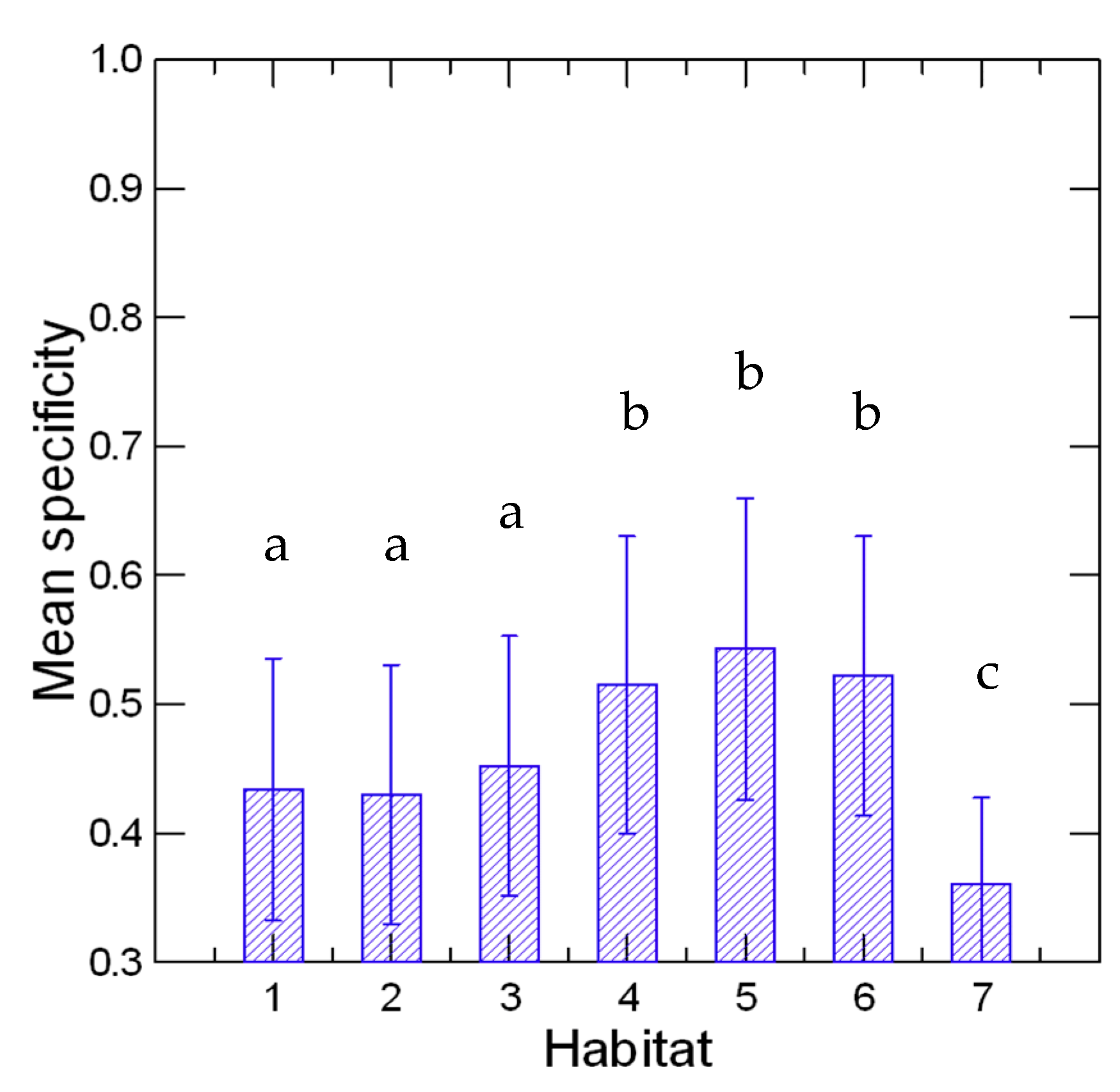
2.6. Habitat Specificity Analysis

An index showing the specificity of each species for each habitat was estimated according to the method proposed by Tylianakis et al. [26]. This index indicates the deviation of the abundance of each species from what would be expected under the null hypothesis of random distribution. The following formula describes in detail the index HSih of species i with habitat h:
H S i h = l o g ( O i j h / E i j h + 1 )
where Oijh and Eijh are the observed and expected number of individuals of species i in plot j, which belongs in habitat h; the expectation is under the null hypothesis of random distribution of the species, which is the total number of individuals of species i in all habitats multiplied by the fraction of individuals of all species found in plot j.
The habitat specificity of insect species was compared across habitats employing a Friedman nonparametric ANOVA [26]. The significance probability is calculated assuming an χ2 distribution for species abundances. The results are tabulated for insect families and family groups since, in general, co-familial species have similar ecological requirements. Whilst the data used in these tests are referred to species, the groups of species are considered here as blocks of cases and the habitats as groups of variables.

2.7. Indicator Species

The determination of diagnostic species was performed by employing the software R package ‘indicspecies’ [60]. The method considers that niche breadth varies among species. In effect, a species would be tested as an indicator of a set of several biotopes, depending on its niche breadth. The method operates on a grouping of biotopes, i.e., plots in this study, obtained with the minimum variance joining method explained in the similarity analysis above. According to Caceres and Legendre [61], the method can interpret the set of sites even in the case where they are characterized by crossed factors [60]. The method was exemplified with a beetle assemblage in a set of sites in which the crossed factors were the wildfire regime (three levels) and the altitude (three levels). The significance of the indication value was assessed with permutations (5000 permutations).
The R package ‘labdsv’ [62] was also employed for verification-only purposes. This package made possible the estimation of the IndVal, i.e., indicator value, of species. The inclusion of a species in both significance-indicator species sets, i.e., found with both packages, strengthens the ability of an insect species to serve as an indicator.

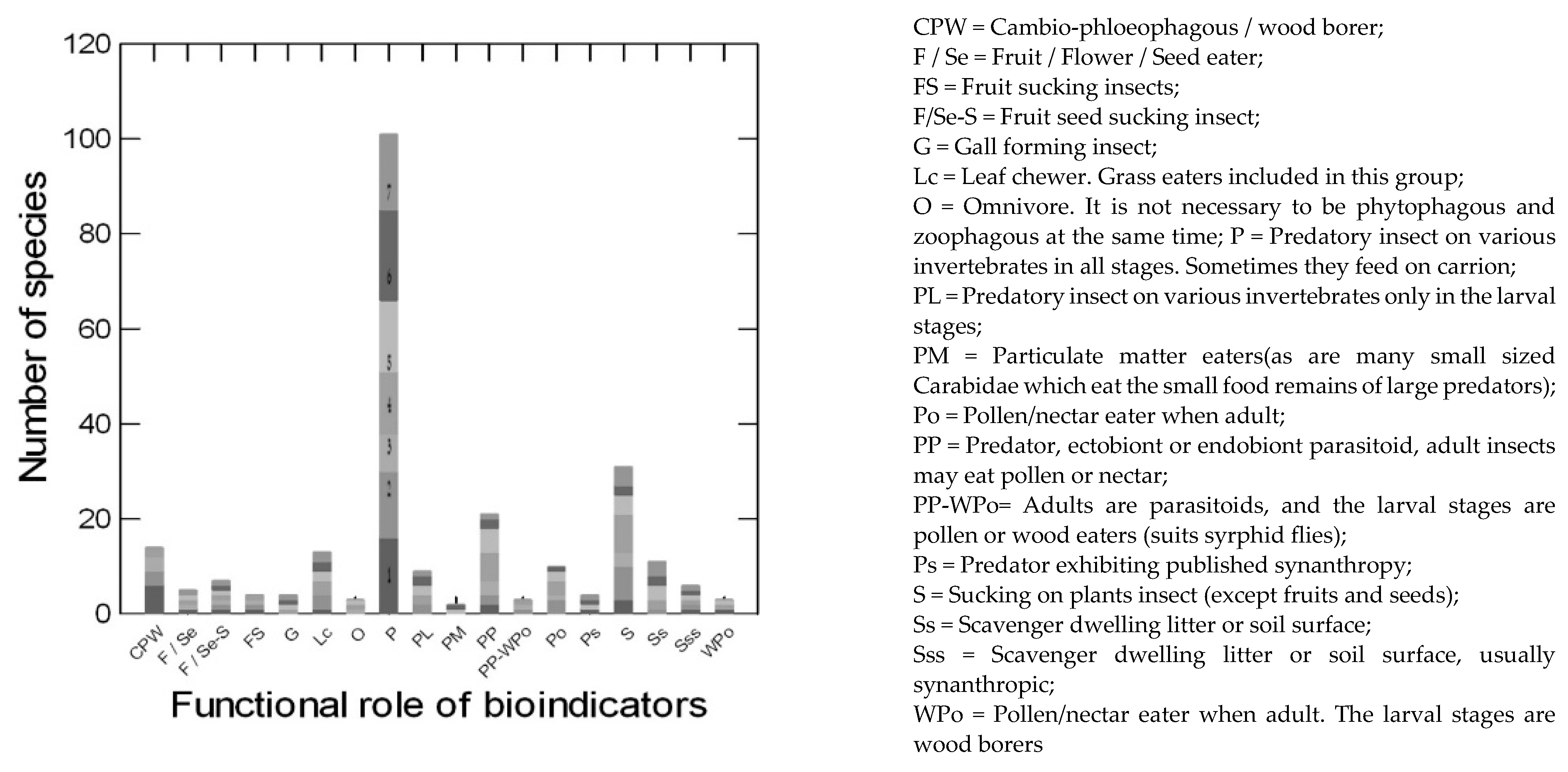
2.8. Functional Roles of Insect Species

Whilst it is known that insect indicator species diagnose habitats, it would be informative if their functional role is used to characterize the impact status of the respective sites. For this purpose, all insect species were categorized into 18 functional roles, and Figure 2 illustrates their numbers in each plant community. These roles are related to the position of each insect in the trophic structure of the eco-system and the way they transform the energy in the feeding substrate [22]. All functional roles are described in Figure 2.
The status of each habitat was measured using three variables commonly used to describe the impact [63] and the specific anthropogenic influences received by the plots. The variables were ‘naturalness’, ‘anthropic elements’, and ‘earthworks’. The last variable is used because of the widespread influence of this activity to cover the needs of the ‘rowing center’. In each plot, a square frame with size 1 m2 was randomly dropped at 12–16 places, depending on the presence of each impact type was recorded by 0/1 notation. Then, the average of the 0/1 triplets was estimated and expressed as a percentage triplet for each plot. We estimated the habitat impact by taking the mean triplet of all constituent plots. The following meanings are attached to the variables: (a) ‘naturalness’ is evidenced when there are (i) old floristic elements, (ii) there are no signs of human presence, (iii) absence of natural exports from forbs, trees, and non-wood products, i.e., the resin of P. halepensis or soil under Pa. lentiscus, and disasters such as forest fires, (iv) absence of fragmentation, (v) presence of laying or standing dead wood; (b) ‘anthropic elements’ are evidenced when (i) there are traces of herb collecting, (ii) human-generated garbage, (iii) past or present human artifacts, (iv) paths generated by browsing sheep/goat flocks, (v) human pathways and traces, and (vi) game traces or hunting remains; (c) ‘earthworks’ are evidenced when soil masses are removed from or brought into the plot, up to 5 years previously. These three impact types are not mutually exclusive, and a specific 1 m2 frame can be characterized by a triplet of 0/1 values summing up to 3, e.g., (0, 1, 1). In essence, the method is similar in the way it measures the three impact measures to the one presented by Hill et al. [64]. However, it operates on a much smaller scale and is adapted to the area of this study.

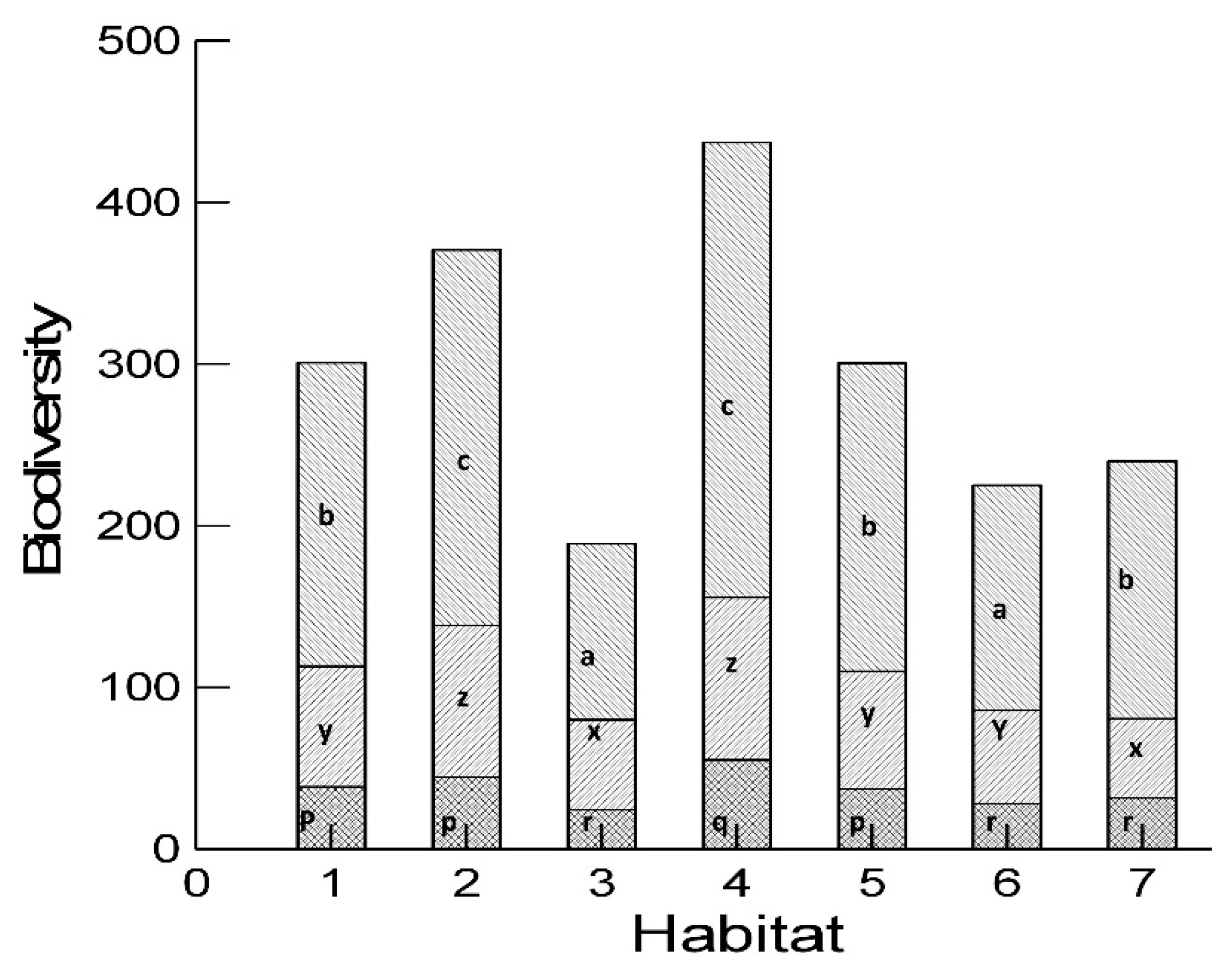
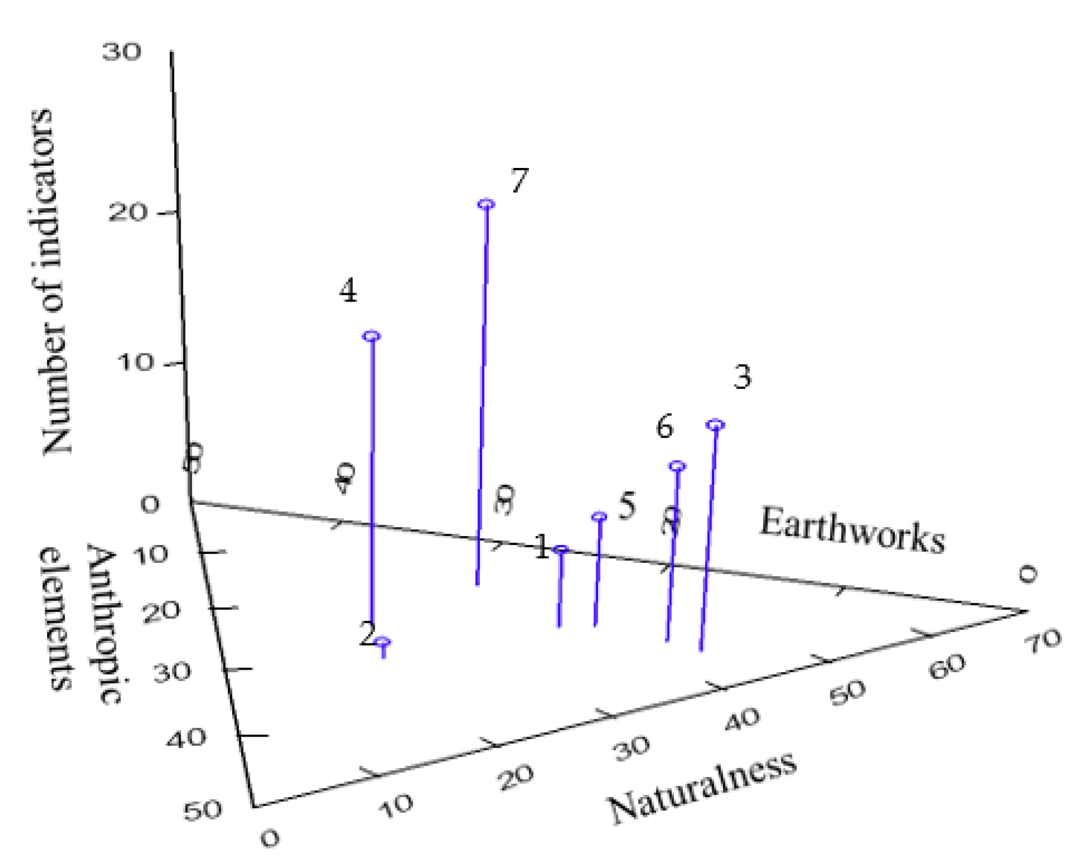
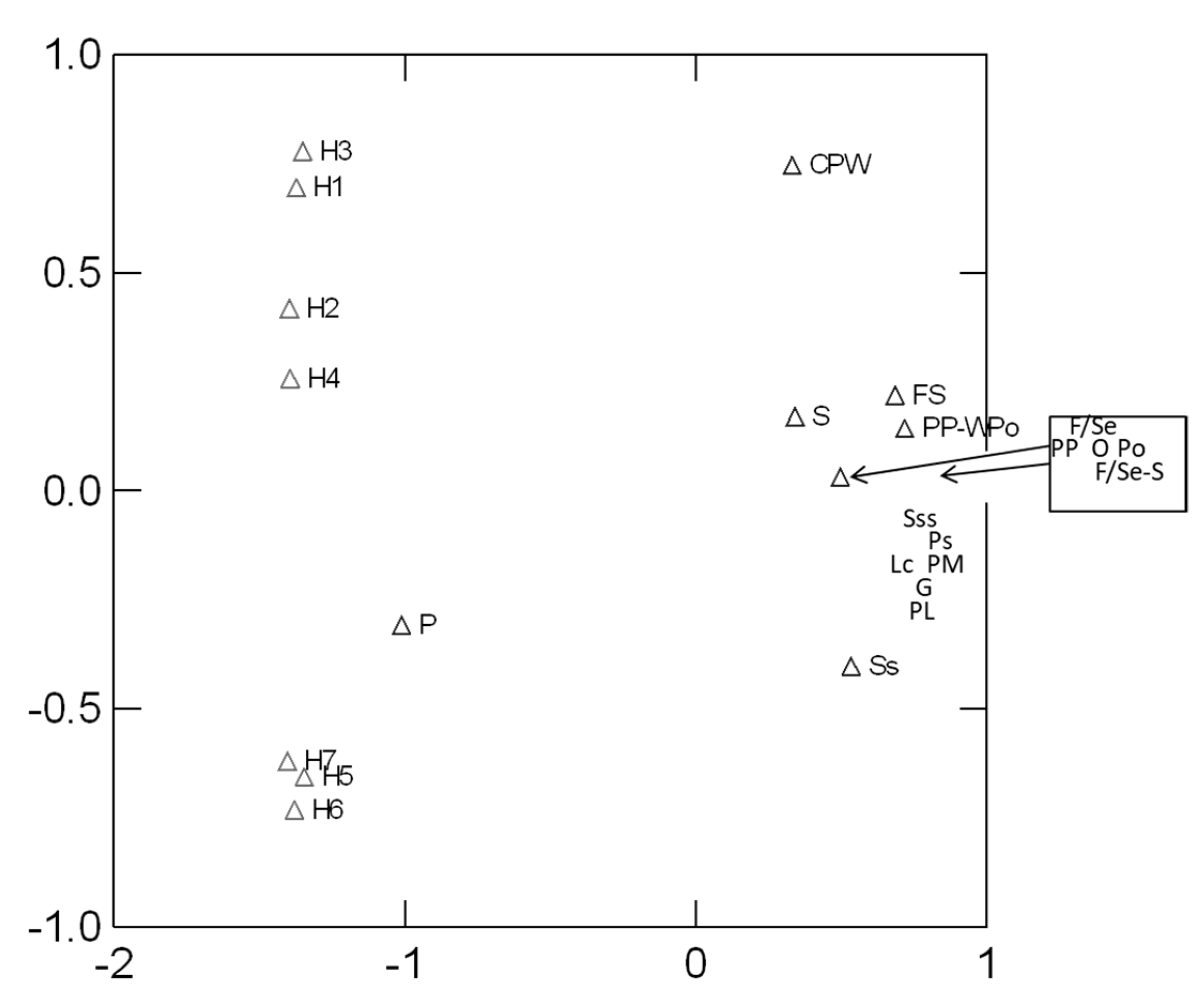
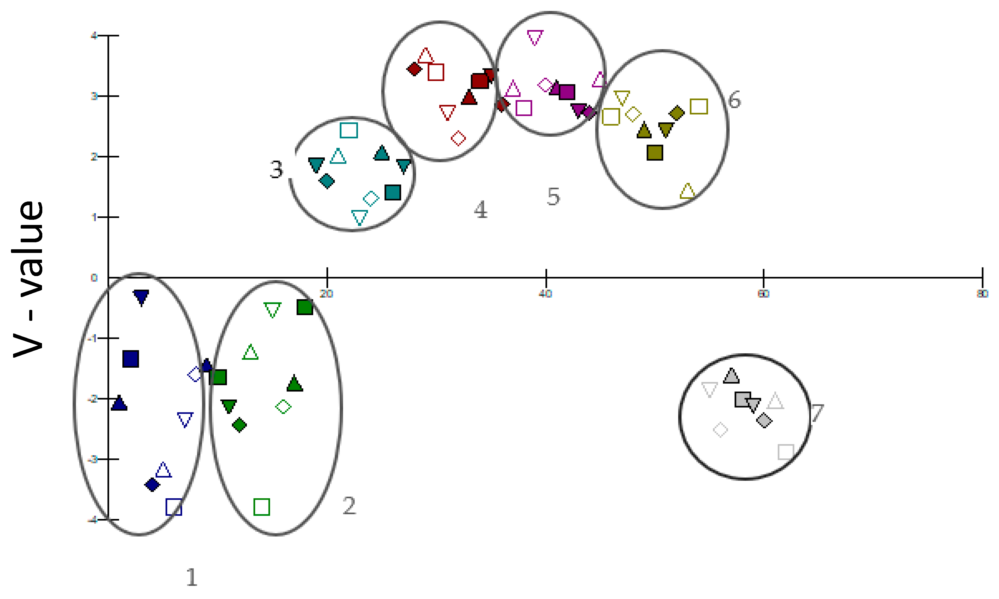
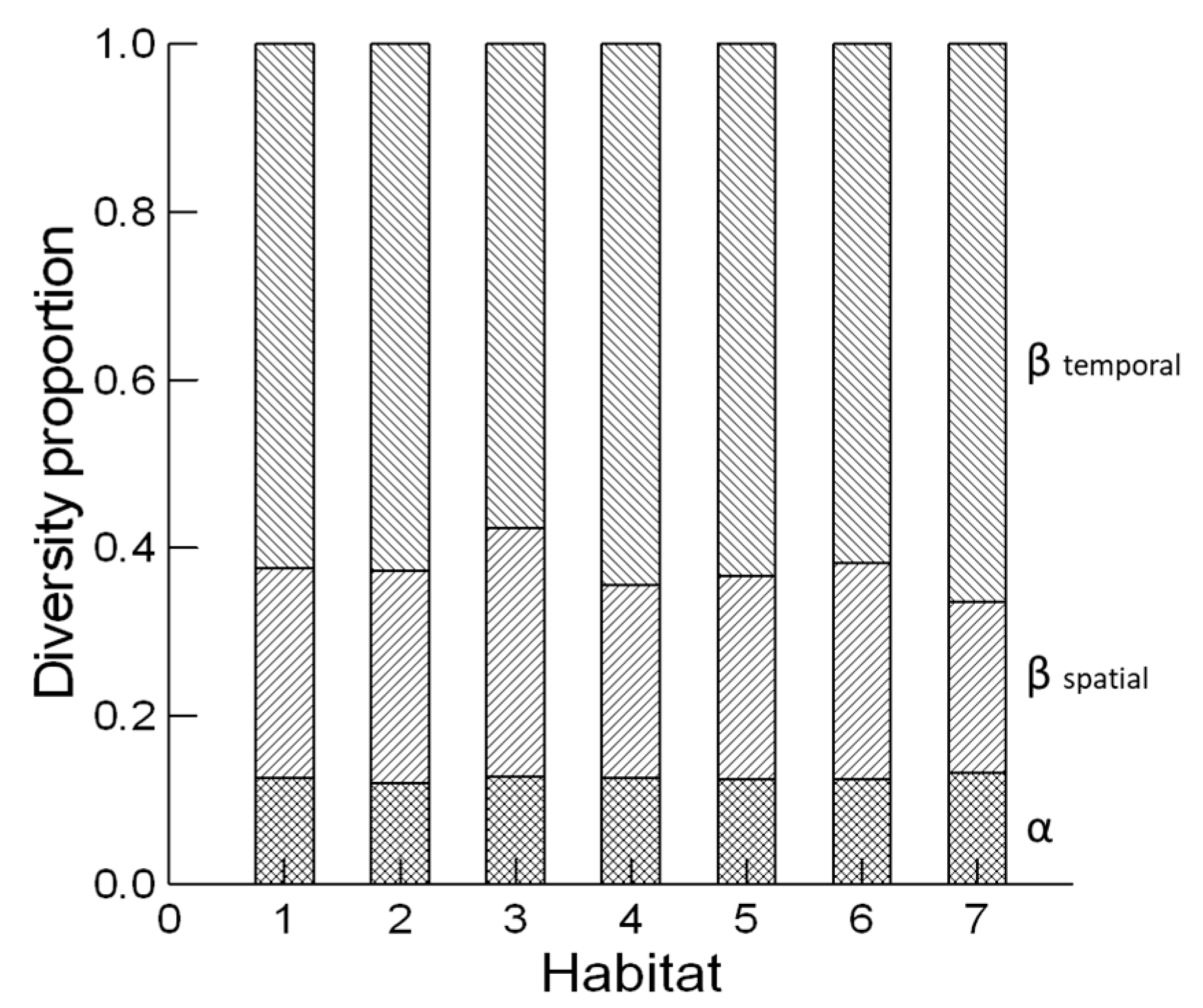
3. Results and Discussion

There are seven habitat types, as indicated by the cluster analysis of the 63 plots. The names and dominant plants of each habitat type are shown in Table 1. A combined NMDS diagram, which includes habitat types as the group indicator, and the functional roles of insects found in the plots, can be seen in Figure A1. The NMDS analysis was successful, with a stress value = 0.02 and a percentage-explained variance of 0.98. In this diagram, the x-axis separates the habitat types from the bulk of insects. Only predatory species (P) fell in the negative x-semiaxis. Importantly, the pine-bearing habitats (H1–H4) were located together in the third quadrant, while the other three habitats H5–H7 fell together in the fourth quadrant. The insects in the CPW (cambio-phloeophagous/wood borer) functional role separated from the rest. All other types, except P, fell together at the far positive end of the x-semiaxis. This diagram shows that there is no preference of any functional role of insects for a habitat type. Only CPW insects behaved differently from the rest and took almost the same y values as pine habitats, accompanied by J. macrocarpa and A. hermaniae. The gradual disappearance of these woody plants from the area removes CPW insects, rather than the spread of P. pinea.
To find the significant associations between the impact type and the functional roles of the bioindicator insect species, we applied the following method. We submitted the matrices of (habitats) × (functional roles of bioindicators) and (habitats) × (impact types and amount) to the ‘adonis’ [65] function of the ‘vegan’ package. This procedure performs a partitioning of the sum of squares, and in this sense, it is analogous to the multivariate analysis of variance. McArdle and Anderson [64] refer to it as a “permutational MANOVA”. This method uses a pseudo-statistic to perform the statistical test of the significance of the interaction of variables describing the habitats of the matrices. It has been used in several ecological works in a mode remarkably similar to redundancy analysis [66].
The Holocene geomorphological evolution of the Schinias area is well-known [27,67,68]. The proposed scenario (Figure 3) includes the initial stage of the formation of an island in front of the plain. It also includes the successive fluvial deposits and sediments, which formed the temporary swamp. The initial profile of the area is a flat-floored depression within karst limestone (marbles). The action of the Makaria and Draconera springs symbolized with ‘x’ at the easternmost edge of the plain (Figure 1) together with the restrictive drainage by surface water courses, gave the area the present configuration (open polje) with an extensive island that has closed the past lagoon (before 3000 BC) bearing a dune system stabilized by pines.
Because of the dunes, these systems are considered protective formations of urban areas [69], while biotic communities on them indicate their status [7,10]. Archaeophytes (established before 1500 AD) indicate relatively undisturbed areas, while neophytes (after 1500 AD) signify human-disturbed dunes. Holocene dunes, such as those found on Schinias, are dominated by archaeophytes, and the insect communities on them are similarly populated by native insects [28,33]. Alien insects prefer dunes among other habitats [7,15]. In Schinias, they prefer stabilized dunes and nearby hilly areas like the ones that surround the pinewood and the marsh in Schinias (Figure 1). From the fact that disturbed dunes offer resources to all types of plants since disturbance creates additional niches for herbivorous insects and their predators, it becomes evident that these habitats cannot be differentiated based on insect species content.
On the other hand, the mean specificity of habitats (Figure 4) and all types of biodiversity (Figure 5) were reduced in P. halepensis- and T. hampeana-dominated habitats. Moreover, the V-statistic shows clearly that these habitats are more disturbed than the more typical habitat of Schinias (Figure 6).
In general, ecologists consider P. halepensis as a post-disturbance pioneer of Mediterranean coastal areas, and records of its recent expansion span over a century of forest surveys in the Mediterranean Basin [70]. This pine replaces P. pinea in all Greek biotopes (e.g., Skiathos Isl. West Peloponnissos) because of a combination of properties, the most important of which is the germination ability immediately after the firing of numerous seeds. Other properties that determine mainly the invasiveness and fire-evader strategy are seroteny (strong in P. halepensis and rare in P. pinea) and early flowering of P. halepensis [71] for invasiveness in South African scrubland [72]. In Schinias, P. halepensis occupied more than 70% of the original P. pinea forest in the 20th century. Although P. halepensis is more susceptible to fire and natural enemies than P. pinea, the previously mentioned ecophysiological properties make the first species able to replace the second from all biotopes where they co-occur [73,74]. Enclosures around seedlings of P. pinea showed that this pine is competitively replaced by the other pine species since it cannot tolerate the shading from the rapidly germinating seedlings of P. halepensis after an ecosystem perturbation (personal observation PVP). The insects associated with the plots where these pines predominate follow this pattern. Plots belonging to habitats 3 and 4 exhibit more specificity than habitats 1 and 2 (Figure 5). This is because P. halepensis invades the sites of P. pinea and removes the insects of P. pinea and the associated shrubs, which are more specialized to cope with the antifeedant essential oils in the resin [73]. For example, the P. pinea phenotype in Schinias is not infested by Marchalina hellenica Gennadius, unlike P. halepensis, because of the sizable percentage of limonene [73]. This causes a momentous change in the entomofauna of plots since the pine scale is followed by scolytids and their natural enemies. In effect, this causes a reduction in the fauna of the ground layer [29]. The concentration of habitats 1, 2, and 4 in the first quarter of the NMDS plain (Figure A1) reflects the condition of the invasion of P. halepensis and the lack of a shrub layer in P. pinea-dominated habitat 3.
The insects that indicate the two P. pinea habitats (3, 4) are more than the ones indicating P. halepensis habitats (1, 2) (Table 1). This proves that the incoming invading pine species does not belong to the Schinias flora. In addition, the insects indicating habitats 1 and 2 are influenced by nearby agricultural activities (C. perla, B. variegator, and E. urozonus) or specializing in exploiting pine tissues (G. staurus pine needles, and T. piniperda cambium and phloem). The insects indicating P. pinea habitats (3 and 4) are predators, but they also include many exploitation niches (e.g., pollen eaters, cambio-phloeophagous, xylophagous, seed eaters, sucking insects, and needle eaters). In both habitat groups, the ripening of pine seeds in the third year (which is unusual among pines) [74] increases the availability of seed resources for exploiting insects and other animals such as rodents and seed-eating passerines. This adds to the replacement of P. pinea by P. halepensis and not by other pine species. Another capability of the P. halepensis is withstanding the lowering of the water table, which is inevitable in the evolution of dunes. Pinus pinea exploits saline water when rainfall water is depleted [75], but P. halepensis, as a drought invader, can withstand even the lowering of brackish and saline water. However, the insect fauna does not follow the replacement in the same time scale, hence the scanty set of indicators (Table A1).
In addition to all these, the nestedness and co-occurrence analysis shows (Table 2) that insect species tended not to co-exist, as indicated by the C-score and CU, which are highly significant. Of course, this can be the outcome of several ecological processes, but here, only the habitat requirements and the competition can be invoked [24,25]. For that reason, the excessive number of predators, as Figure 2 and Table A1 show, cannot suppress the populations of herbivorous insects.
The other three habitats (5, 6, and 7) had a similarly large number of bioindicators with 11, 7, and 24 insect species, respectively. We can observe the superficial paradox that many insects indicate the heavily impacted habitat 7. Even if the three T. hampeana monophagous insects are removed (T. tamaricicola, O. stictogalus, and C. tamaricis), 21 species remain as habitat 7 indicators. Not all insects are freshwater specialists, such as A. imperator, S. falleni, G. lacustris, H. sahlbergi, and C. lateralmarginalis. Among them, L. decipiens, B. mucronata, O. olens, and Quedius sp. are detritivorous or occasionally carcass eaters or even predators, and the other insects belong to a variety of niches. They were found in the macchia and pseudomacchia vegetation on the hills that border Schinias. This means either that most insect indicators are coming from other nearby areas and avoid the other habitats, or that T. hampeana prefers to grow on advanced dune successional stages, which harbor a multitude of specialized indicators [16]. In addition, habitat 7 has the highest α and βΤ diversities and the lowest βS diversity. This means that there is a high turnover of species that increases the richness of the plots. However, these insects are very mobile and do not differentiate plots from one another. This fact is also responsible for the low mean specificity of this habitat, together with the fact that T. hampeana insects occupy trees in all plots of the habitat.
Habitat 7 received the bulk of earthworks from the construction phase of the ‘canoeing and rowing center’. As a result, it is expected to bear pioneer herbs and grasses and all the insects associated with herbaceous (though not exclusively) vegetation like E. fasciata, N. aduncus, R. consors, and L. macaronius. As a result, the diversity is expected to be based on time rather than on space, hence the proportionally lowest βS and the proportionally highest βΤ (Figure 7) but the lowest overall γ diversity (=βS + α) (Figure 5).
Regarding the functional roles of insect bioindicators, the number of bioindicators (Figure 8) was not related to the impact status of the habitat. It is the taxonomic status of the plant that grows and dominates the habitat, rather than its status, which configures the number of bioindicators. In effect, habitat 7 dominated by T. hampeana bears the unique entomofauna of this taxonomically isolated tree that can grow on recently imported soils from other sites in the area. Almost all insect species found on this tree are within the group of bioindicators of habitat 7 (Table A1).
Habitats 3 and 4 with P. pinea and the old habitats 5 and 6, which are closer to the natural vegetation of Schinias according to Figure 6 and Figure 2, harbored the highest numbers of parasitoid and sucking insects.
The measures of the disturbance of the habitats interacted significantly, as is the case of most of the proposed measures. These measures are complicated quantities estimated from disturbed biological communities [64]. Because of this, it is difficult to find a prominent pattern except for the one found in the previous paragraph. For instance, from the predatory trophic level, only parasitoids (PP), predators at larval stages (PL), and synanthropic predators (Ps) differed significantly among habitats, unlike all-stage predators (P). Workers on the composition patterns of a river catchment Heteroptera, in Hungary, stated that the distribution pattern of predaceous Heteroptera could be influenced by various factors [76] eventually, not solely by the ones measured in this study. On the other hand, in the small scale of this study, the successional status of a particular plot may be disturbed by summer visitors who walk on paths under the old P. pinea trees. This creates early successional vegetation stages mingled with the late ones. So, the insects of the respective plots are influenced by disturbed succession in addition to interrupted connectivity.
The vicinity of the area to agricultural land further complicates the analysis since there are many corridors that mix the entomofauna. In this way, the specificity of each habitat, both in terms of species and in 18 functional roles, is severely reduced. The reduction in the vegetation is behind the spread of grass-dominated corridors within all habitats in Schinias. The development of understory shrubs is perhaps a defense of the existing plants. These grassland corridors and dikes (of a river system instead of a marsh) were also found to be important insect corridors that enlarge habitats and reduce fragmentation [76]. On the other hand, grassland corridors are probably early secondary successional stages or primordial revegetated fragmentation [77] and do not increase the colonization of plots, which becomes zero by rare species [78]. In this sense, grassland corridors do not directly affect the constitution of habitats in functional insect types. The influence of corridors is exerted solely through the reduction in vegetation.

4. Conclusions

In conclusion, the pinewood and marsh area at Schinias receives ongoing human impact in many forms. (a) Urbanization is prominent in the area between the marsh and pinewood and the northern part. This changed insect communities both in terms of constituent insect species and their abundance. These changes were mediated by changing the plant communities of Schinias. (b) Tourism-related construction was evidenced in the ‘canoeing and rowing center’ in the western part, but the earthworks were transported all over the area. These activities also changed the insect communities in a qualitative and quantitative sense. The results showed that no insect species can solely respond to the per se construction works. An exception is perhaps the CPW (cambio-phloeophagous and wood-boring) insects, which were associated with P. halepensis and avoided P. pinea. (c) Finally, the restriction of the marsh seems to change the entomofauna of habitats. It is done either directly by both changing the marsh vegetation and favoring the replacement of P. pinea by P. halepensis or by creating open ground that is covered by P. halepensis seedlings. In addition, it lowers the water table. This last event is a prerequisite for the germination of P. pinea seeds. (d) Finally, the indicator values of insect species show what functional roles of insects are important indicators in each plant community.
The implementation of conservation tools in the area and their dynamic adaptation to local social conditions seem crucial. This degraded biotope must be rehabilitated through ecological management to guarantee long-term sustainability and the maintenance of its ecosystem services. Additionally, the rehabilitation must consider the socioeconomic, political, and cultural needs. The lessons from Schinias can be extended to other P. pinea forests since all area habitats share a common natural history.

Author Contributions

Conceptualization, P.V.P., P.P.K. and A.D.S.; methodology, P.V.P.; software, P.V.P.; validation, P.V.P., I.S., K.S. and A.F.; formal analysis, P.V.P.; investigation, all authors; resources, P.V.P., P.P.K. and I.S.; data curation, P.P.K. and A.D.S.; writing—original draft preparation, P.V.P., P.P.K. and A.D.S.; writing—review and editing, P.V.P. and P.P.K.; visualization, P.P.K. and A.D.S.; supervision, P.V.P.; project administration, P.V.P., K.S. and I.S.; funding acquisition, P.V.P. All authors have read and agreed to the published version of the manuscript.

Funding

This research was partly funded by the EU program “Greece-Korea: Secondary metabolites of Hypericum species”, and the Hellenic Ministry of Food and Rural Development program of ‘Surveys 2009–2012 of quarantine organisms’.

Institutional Review Board Statement

Not applicable.

Informed Consent Statement

Not applicable.

Data Availability Statement

All data used in this study can be found in the Institute of Mediterranean Forest Ecosystems, ELGO-Demeter.

Acknowledgments

Theodoros Kritikos and Kosmas Albanis are thanked for helping in data collection and mist-blowing operations. Thanks, are also due to Anastasios Legakis, Yiannis Anastasiou, Apostolis Trihas, Spyros Sphendourakis, Sinos Giokas, George Karetsos, Valia Daskalakou, Kostas Thanos, the mayor of the city of Marathon Spyros Zaggaris, the authority of Kato Souli village Themistocles Anastasiadis, the late shepherd Pandos, and all students and foresters who aided in sampling and talking. Vassilios Roussis and the late Costas Vagias helped in many good overnight discussions. The late Sakis Drosopoulos contributed to many parts of insect identification. Funds for this work came from the Hellenic Ministry of the Environment, the Secretariat for Research and Technology, EU program ‘Greece-Korea: Secondary metabolites of Hypericum species, and the Hellenic Ministry of Food and Rural Development program of ‘Surveys 2009–2012 of quarantine organisms’.

Conflicts of Interest

The authors declare no conflict of interest.

Appendix A

Table A1. Insect species that are significant indicators of plot groups. Eighty species out of 140 are significant indicators and are shown in this table. The probability of having a smaller indicator value is 0.05 or smaller. The last column describes the functional role of each insect species. The explanations of symbols are given in Figure 2.
Site GroupInsect SpeciesIndicator Value
(Higher for ‘Good’ Indicator)
P Functional Role
1Grypotes staurus0.6950.02*S
Tomicus piniperda0.6930.043*CPW
Lionychus (Lionychus) quadrillum0.6170.021*P
Chrysopa perla0.5730.038*PL
Bracon variegator0.5240.002**PP
2Eupelmus urozonus0.6180.045*PP
3Acupalpus (Acupalpus) maculatus1.0000.001***P
Rhagium (Rhagium) inquisitor1.0000.001***CPW
Pissodes (Pissodes) gyllenhali1.0000.001***CPW
Raphidia (Raphidia) ophiopsis mediterranea1.0000.001***P
Mantis religiosa1.0000.001***P
Ulrike attica0.80.008**P
Acanthocinus reticulatus0.7980.001***CPW
Orthotomicus erosus0.7580.029*CPW
Trechus (Trechus) subnotatus0.730.001***Ps
Bacillus atticus0.7270.02*Lc
Panorpa germanica graeca0.720.015*P
Dromius (Dromius) agilis0.6880.001***P
Melanophila cuspidata0.6820.036*CPW
Anthaxia (Melanthaxia) corinthia0.6320.039*WPo
4Brachymeria tibialis1.0000.001***PP
Clanoptilus (Clanoptilus) elegans0.8280.001***Po
Urophora cardui0.8060.001***G
Tentyria rotundata0.7640.001***Ss
Dolichomitus sericeus0.7140.023*PP
Bombus terrestris0.7020.023*Po
Chorthippus (Glyptobothrus) brunneus brunneus0.6960.015*Lc
Scaeva albomaculata0.690.012*PL
Lygaeus pandurus ssp. pandurus0.6870.016*FS
Philaenus spumarius0.6750.01**S
Ancyrosoma leucogrammes0.6640.007**S
Loxocnemis dentator0.6590.044*S
Centrocoris spiniger0.6570.048*S
Staria lunata0.6510.049*S
Messsor sp. 0.6210.029*S
Oedemera (Oedemera) flavipes0.6180.048*Po
Hypophloeus linearis0.5850.039*P
Calathus (Calathus) fuscipes graecus0.5370.015*P
5Lestes barbarus1.0000.001***P
Sympetrum striolatum1.0000.001***P
Libellula depressa1.0000.001***P
Chironomus sp. 1.0000.001***PM
Sympetrum meridionale0.7870.001***P
Lissonota (Loxonota) histrio0.7260.001***PP
Sympetrum fonscolombii0.7230.001***P
Dasypogon melanopterus0.7150.001***P
Hypera sp. 0.680.023*Lc
Harpalus (Artabas) dispar splendens0.5760.022*O
Pimelia (Camphonota) subglobosa0.5450.037*Sss
6Syromastus rhombeus0.8720.001***F/Se
Henestaris halophilus0.8420.001***Se
Aphaenogaster subterranea0.8380.001***O
Trichograma sp. 0.8150.001***PP
Paragus tibialis0.7270.004**PP-WPo
Diadegma trochanteratum0.6790.027*PP
Ischnura elegans0.6320.036*P
7Anax imperator1.0000.001***P
Opsius stactogalus1.0000.001***S
Tuponia tamaricicola1.0000.001***S
Notonecta (Notonecta) maculata1.0000.001***P
Myopa buccata1.0000.001***PP-WPo
Coniatus (Coniatus) tamarisci0.9880.001***F/Se
Loboptera decipiens0.9540.001***Ss
Sigara (Subsigara) falleni0.9480.001***P
Calomera littoralis nemoralis0.870.001***P
Dociostaurus maroccanus0.8660.001***Lc
Hesperocorixa sahlbergi0.8530.001***P
Gerris (Gerris) costae fieberi0.8120.001***P
Empusa fasciata0.810.001***P
Neides aduncus0.7460.001***S
Acinopus (Acinopus) subquadratus0.7450.001***P
Cephalota (Taenidia) circumdata circumdata0.7350.001***P
Libelloides macaronius0.720.001***P
Blaps mucronata0.6920.001***Ss
Aciura coryli0.6890.001***F
Carabus (Tomocarabus) convexus0.6470.001***P
Ocypus (Ocypus) olens0.6040.036*P
Quedius sp. 0.5920.023*P
Cybister (Scaphinectes) lateralimarginalis0.5450.048*P
Rhyparochromus consors0.5180.001***F/Se-S
*** p < 0.001; ** p < 0.01; * p < 0.05.
Figure A1. Diagram of the non-metric multidimensional analysis of habitats and the functional roles of insects according to their insect species content. The diagram space is partitioned in four quadrants. The bulk of the functional roles fall to the positive x-semiaxis. Habitats H1-H4 fall in the second and the rest of habitats fall in the third one together with the predatory insects.
Forests 14 00392 g0a1
Figure A2. Brief photos of important plants and their habitats at Schinias: 1. Elymus farctus, 2. Echium arenarium, 3. Salicornia fruticose, 4. Limonium bellidifolium, 5. Juniperus phoenicea, 6. Pistacia lentiscus, 7. Lagurus ovatus, 8. Trifolium campestre, 9. Pinus pinea, 10. Pinus halepensis, 11. Smilax aspera, 12. Cistus criticus, 13. Piptatherum miliaceum, 14. Brachypodium retusum, 15. Muscari commosum, and 16. Erodium cicutarium (photo credit: A. solomou).
Forests 14 00392 g0a2

References

  1. Martínez, J.; Psuty, N.P. (Eds.) Coastal Dunes: Ecology and Conservation; Springer: Berlin/Heidelberg, Germany, 2004. [Google Scholar]
  2. Everard, M.; Jones, L.; Watts, B. Have We Neglected the Societal Importance of Sand Dunes? An Ecosystem Services Perspective. Aquat. Conserv. Mar. Freshw. Ecosyst. 2010, 20, 476–487. [Google Scholar] [CrossRef]
  3. Vassallo, P.; Paoli, C.; Fabiano, M. Ecosystem Level Analysis of Sandy Beaches Using Thermodynamic and Network Analyses: A Study Case in the NW Mediterranean Sea. Ecol. Indic. 2012, 15, 10–17. [Google Scholar] [CrossRef]
  4. Rust, I.C.; Illenberger, W.K. Coastal dunes: Sensitive or not? Landsc. Urban Plan. 1996, 34, 165–169. [Google Scholar] [CrossRef]
  5. Sýkora, K.; van den Bogert, J.C.J.M.; Berendse, F. Changes in soil and vegetation during dune slack succession. J. Veg. Sci. 2004, 15, 209–218. [Google Scholar] [CrossRef]
  6. Spanou, S.; Verroios, G.; Dimitrellos, G.; Tiniakou, A.; Georgiadis, T. Willdenowia, Bd. 36, H. 1; Special Issue: Festschrift Werner; Botanic Garden and Botanical Museum: Berlin, Germany, 2016; pp. 235–246. [Google Scholar]
  7. Acosta, A.; Carranza, M.L.; Izzi, C.F. Community types and alien species distribution in Italian coastal dunes. In Biological Invasions: From Ecology to Conservation; Rabitsch, W., Essl, F., Klingenstein, F., Eds.; Pensof Publishers: Sofia, Bulgaria, 2007; pp. 96–104. [Google Scholar]
  8. Clarke, D.; Sanitwong Na Ayutthaya, S. Predicted Effects of Climate Change, Vegetation and Tree Cover on Dune Slack Habitats at Ainsdale on the Sefton Coast, UK. J. Coast. Conserv. 2010, 14, 115–125. [Google Scholar] [CrossRef]
  9. Psuty, N.P.; Silveira, T.M. Global Climate Change: An Opportunity for Coastal Dunes? J. Coast. Conserv. 2010, 14, 153–160. [Google Scholar] [CrossRef]
  10. Weeda, E.J. The Role of Archaeophytes and Neophytes in the Dutch Coastal Dunes. J. Coast. Conserv. 2010, 14, 75–79. [Google Scholar] [CrossRef] [Green Version]
  11. Diogo, A.C.; Vogler, A.P.; Gimenez, A.; Gallego, D.; Galian, J. Conservation genetics of Cicindeladeserticoloides, an endangered tiger beetle endemic to southeastern Spain. J. Insect Conserv. 1999, 3, 117–123. [Google Scholar] [CrossRef]
  12. Maes, D.; Ghesquiere, A.; Logie, M.; Bonte, D. Habitat Use and Mobility of Two Threatened Coastal Dune Insects: Implications for Conservation. J. Insect Conserv. 2006, 10, 105–115. [Google Scholar] [CrossRef]
  13. Salz, A.; Fartmann, T. Coastal Dunes as Important Strongholds for the Survival of the Rare Niobe Fritillary (Argynnis niobe). J. Insect Conserv. 2009, 13, 643–654. [Google Scholar] [CrossRef]
  14. Rooney, P. Changing Perspectives in Coastal Dune Management. J. Coast. Conserv. 2010, 14, 71–73. [Google Scholar] [CrossRef] [Green Version]
  15. Howe, M.A.; Knight, G.T.; Clee, C. The importance of coastal sand dunes for terrestrial invertebrates in Wales and in the UK, with particular reference to aculeate Hymenoptera (bees, wasps & ants). J. Coast. Conserv. 2010, 14, 91–102. [Google Scholar]
  16. Wünsch, Y.; Schirmel, J.; Fartmann, T. Conservation Management of Coastal Dunes for Orthoptera Has to Consider Oviposition and Nymphal Preferences. J. Insect Conserv. 2012, 16, 501–510. [Google Scholar] [CrossRef]
  17. Choi, Y.D.; Temperton, V.M.; Allen, E.B.; Grootjans, A.P.; Halassy, M.; Hobbs, R.J.; Naeth, M.A.; Torok, K. Ecological Restoration for Future Sustainability in a Changing Environment. Ecoscience 2008, 15, 53–64. [Google Scholar] [CrossRef]
  18. Economidou, E. The Attic Landscape throughout the Centuries and Its Human Degradation. Landsc. Urban Plan. 1993, 24, 33–37. [Google Scholar] [CrossRef]
  19. Dafis, S.; Papastergiadou, K.; Georghiou, D.; Babalonas, T.; Georgiadis, T.; Papageorgiou, M.; Lazaridou, T.; Tsiaousi, V. Directive 92/43/EEC The Greek “Habitat” Project NATURA 2000: An overview. In Life Contract B4-3200/94/756, Commission of the European Communities DG XI; The Goulandris Natural History Museum-Greek Biotope/Wetland Centre: Athens, Greece, 1996. [Google Scholar]
  20. Stewart, A.J.A.; New, T.R. Insect Conservation in temperate biomes; issues, progress and prospects. In Insect Conservation Biology; Stewart, A.J.A., New, T.R., Lewis, O.T., Eds.; Proceedings of the Royal Entomological Society: London, UK, 2007; pp. 1–33. [Google Scholar]
  21. Schaffers, A.P.; Raemakers, I.P.; Sykora, K.V.; ter Braak, C.J.F. Arthropod Assemblages Are Best Predicted By Plant. Ecology 2008, 89, 782–794. [Google Scholar] [CrossRef]
  22. Speight, M.R.; Hunter, M.D.; Watt, A.D. Ecology of Insects: Concepts and Applications; Wiley-Blackwell: Oxford, UK, 2008. [Google Scholar]
  23. Feest, A.; Eyre, M.D.; Aldred, T.D. Measuring carabid beetle biodiversity quality: An example of setting baseline biodiversity indices. Curr. Trends Ecol. 2011, 2, 11–23. [Google Scholar]
  24. Carvalho, J.C.; Cadoso, P.; Cespo, L.C.; Henriques, S.; Carvalho, R.; Gomes, P. Biogeogrphic paterns of spiders in coastal dunes along a gradient of mediterraneity. Biodivers. Conserv. 2011, 20, 873–894. [Google Scholar] [CrossRef]
  25. Spanos, K.A.; Petrakis, P.V.; Daskalakou, E. Salient points on the assessment and monitoring of forest biodiversity. Bioremedation Biodivers. Bioavailab. 2010, 4, 1–7. [Google Scholar]
  26. Tylianakis, J.M. Spatiotemporal variation in the diversity of Hymenoptera across a tropical habitat gradient. Ecology 2005, 86, 3296–3302. [Google Scholar] [CrossRef] [Green Version]
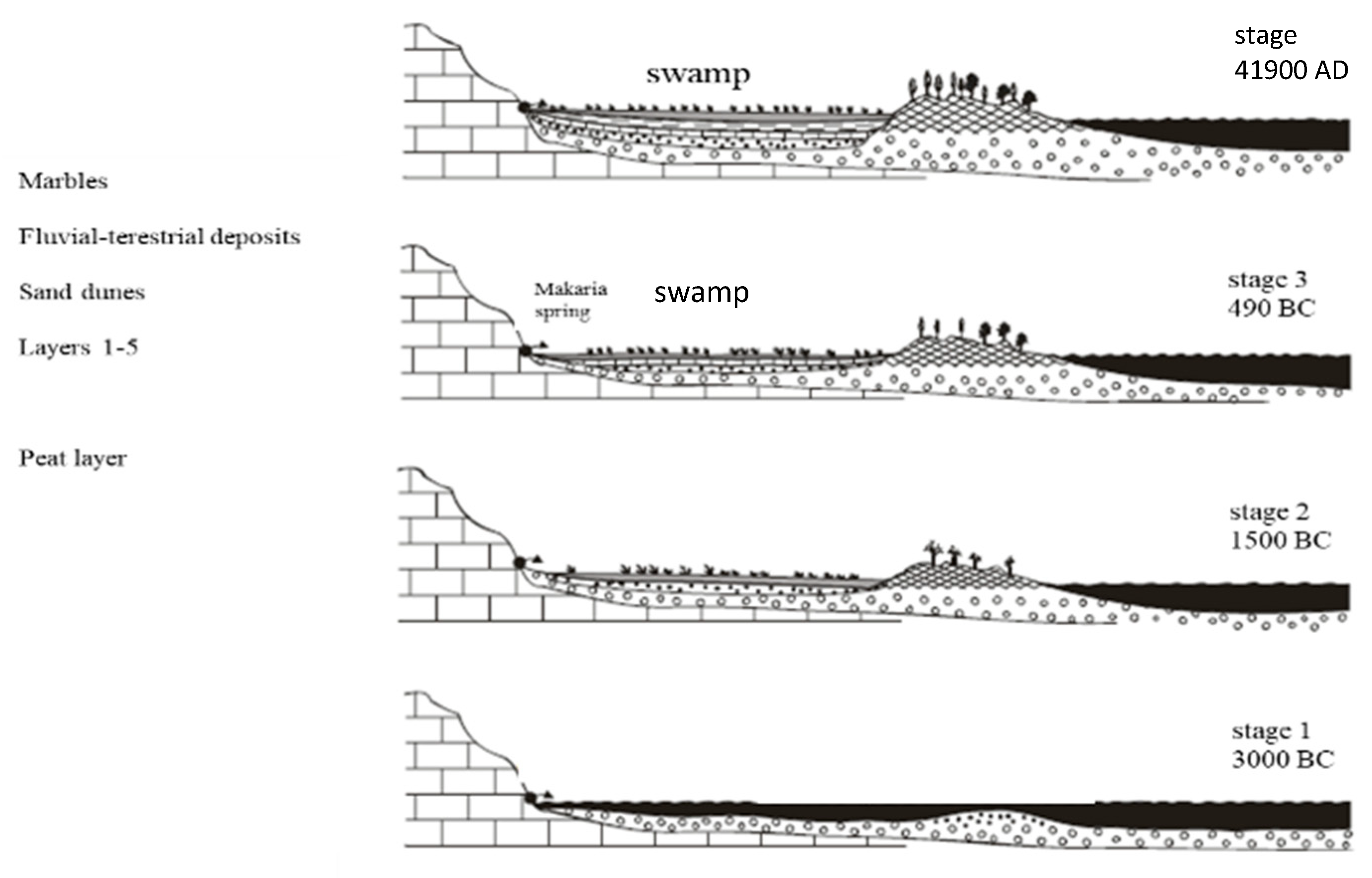
  27. Pavlopoulos, K.; Karkanas, P.; Triantaphyllou, M.; Karymbalis, E.; Tsourou, T.; Palyvos, N. Paleoenvironmental Evolution of the Coastal Plain of Marathon, Greece, during the Late Holocene: Depositional Environment, Climate, and Sea Level Changes. J. Coast. Res. 2006, 22, 424–438. [Google Scholar] [CrossRef]
  28. Petrakis, P.V. Plant–Heteroptera Associations in an East -Mediterranean Ecosystem: An Analysis of Structure, Specificity and Dynamics. Ph.D. Thesis, University of Cardiff, Wales, UK, 1991. [Google Scholar]
  29. Petrakis, P.V.; Spanos, K.; Feest, A. Insect Biodiversity Reduction of Pinewoods in Southern Greece Caused by the Pine Scale (Marchalina hellenica). For. Syst. 2011, 20, 27. [Google Scholar] [CrossRef] [Green Version]
  30. Knott, P.; Warren, A. Aeolian processes. In Geomorphological Techniques; Goudie, A., Ed.; George Allen and Unwin: London, UK, 1981; pp. 226–246. [Google Scholar]
  31. Diapoulis, C. The Hellenic Flora: Identification Keys of Greek Plants; University of Athens: Athens, Greece, 1949. (In Greek) [Google Scholar]
  32. Economidis, P.S. Check List of Freshwater Fishes of Greece; Hellenic Society for the Protection of Nature: Athens, Greece, 1991. [Google Scholar]
  33. Gaitlich, M.; Dragoumis, F. The Ecological Value of Small Wetlands; Bulletin of the Hellenic Ornithological Society: Athens, Greece, 1985; Issue 2. (In Greek) [Google Scholar]
  34. Spanou, S.; Tiniakou, A.; Nikolaidis, V.; Georgiadis, T. Comparative study of protected areas in Greece: The case-study of three littoral Pinus pinea (stone pine) forests. Fresenius Env. Bull 2007, 16, 1335–1344. [Google Scholar]
  35. Alinvi, O.; Ball, J.P.; Danell, K.; Hjältén, J.; Pettersson, R.B. Sampling Saproxylic Beetle Assemblages in Dead Wood Logs: Comparing Window and Eclector Traps to Traditional Bark Sieving and a Refinement. J. Insect Conserv. 2007, 11, 99–112. [Google Scholar] [CrossRef]
  36. Southwood, T.R.E.; Henderson, P.A. Ecological Methods: With Particular Reference to the Study of Insect Populations; Blackwell Science: Oxford, UK, 2000. [Google Scholar]
  37. Floren, A.; Gogala, A. Heteroptera from beech (Fagus sylvatica) and silver fir (Abies alba) trees of the primary forest reserve RajhenavskiRog, Slovenia. Acta Entomololica Slov. 2002, 10, 25–32. [Google Scholar]
  38. Ozanne, C.M.P. Techniques and methods for sampling canopy insects. In Insect Sampling in Forest Ecosystems; Leather, S., Ed.; Blackwell Publishing: Hoboken, NJ, USA, 2005; pp. 146–167. [Google Scholar]
  39. Novotný, V.; Basset, Y. Rare species in communities of tropical insect herbivores: Pondering the mystery of singletons. Oikos 2000, 89, 564–572. [Google Scholar] [CrossRef] [Green Version]
  40. De Jong, Y.S.D.M. (Ed.) Fauna Europaea Version 2.4.Web Service. Available online: http://www.faunaeur.org/ (accessed on 15 October 2011).
  41. Aber, J.D. A Method for Estimating Foliage-Height Profiles in Broad-Leaved Forests. J. Ecol. 1979, 67, 35–40. [Google Scholar] [CrossRef]
  42. Orloci, L.; Rao, C.R.; Stiteler, W.M. (Eds.) Multivariate Methods in Ecological Work, Statistical Ecology; ICPH: Fairland, MD, USA, 1979; Volume 7. [Google Scholar]
  43. Wilkinson, L. SYSTAT 12: The System for Statistics; SYSTAT Software Inc.: Evanston, IL, USA, 2007. [Google Scholar]
  44. Kruskal, J.B.; Wish, M. Multidimensional Scaling; Sage Publ.: Beverly Hills, CA, USA, 1978. [Google Scholar]
  45. Clarke, K.R.; Green, R.H. Statistical design and analysis of a biological effects study. Mar. Ecol. Prog. Ser. 1988, 46, 213–226. [Google Scholar] [CrossRef]
  46. Clarke, K.R.; Somerfield, P.J.; Chapman, M.G. On Resemblance Measures for Ecological Studies, Including Taxonomic Dissimilarities and a Zero-Adjusted Bray-Curtis Coefficient for Denuded Assemblages. J. Exp. Mar. Biol. Ecol. 2006, 330, 55–80. [Google Scholar] [CrossRef]
  47. Lasiak, T. Influence of taxonomic resolution, biological attributes and data transformations on multivariate comparisons of rocky macrofaunal assemblages. Mar. Ecol. Prog. Ser. 2003, 250, 29–34. [Google Scholar] [CrossRef] [Green Version]
  48. Oksanen, J.; Blanchet, F.G.; Kindt, R.; Legendre, P.; Minchin, P.R.; O’Hara, R.B.; Simpson, G.L.; Solymos, P.; Stevens, M.H.H.; Wagner, H. Package ‘vegan’: Community Ecology Package. Version 2.0-0. Available online: https://cran.r-project.org/web/packages/vegan/vegan.pdf (accessed on 18 December 2011).
  49. R Development Core Team. R: A Language and Environment for Statistical Computing; R Foundation for Statistical Computing: Vienna, Austria; ISBN 3-900051-07-0. Available online: http://www.R-project.org/ (accessed on 18 December 2011).
  50. Magurran, A.E. Measuring Biological Diversity. Blackwell, Oxford, UK Management Board of Schinias Marathon National Park. 2021. Technical Report. Installation of a Pilot Network of Experimental Surfaces and Regeneration Centers for the restoration of the Pine Forest in the Schinias—Marathon National Park through the Enrichment of Gaps and the Enhancement of Biodiversity (flora), and the Natural Regeneration with Various Methods. 2004, p. 48. Available online: https://www.greekflora.gr/el/Default.aspx (accessed on 12 December 2022).
  51. Lambshead, P.J.D.; Platt, H.M. Analysis of disturbance with the Ewens/Caswell neutral model: Theoretical review and practical assessment. Mar. Ecol. Prog. Ser. 1988, 43, 31–41. [Google Scholar] [CrossRef]
  52. Karakassis, I.; Smith, C.J.; Eleftheriou, A. Performance of neutral model analysis in a spatiotemporal series of macrobenthic replicates. Mar. Ecol. Prog. Ser. 1996, 137, 173–179. [Google Scholar] [CrossRef]
  53. McAleece, N. BioDiversity Professional. The Natural History Museum and The Scottish Association for Marine Science 1997. Available online: http://www.nhm.ac.uk/zoology/bdpro/ (accessed on 10 February 2012).
  54. Ulrich, W. NODF—A FORTRAN Program for Nestedness Analysis, Version 1.0; Nicolaus Copernicus University: Torun, Poland, 2010. [Google Scholar]
  55. Wright, D.H.; Reeves, J.H. On the meaning and measurement of nestedness of species assemblages. Oecologia 1992, 92, 416–428. [Google Scholar] [CrossRef] [PubMed]
  56. Kerr, J.T.; Sugar, A.; Packer, L. Indicator Taxa, Rapid Biodiversity Assessment, and Nestedness in an Endangered Ecosystem. Conserv. Biol. 2000, 14, 1726–1734. [Google Scholar] [CrossRef]
  57. Almeida-Neto, M.; Guimaraes, P.; Guimaraes, P.R., Jr.; Loyola, R.D.; Ulrich, W. A consistent metric for nestedness analysis in ecological systems: Reconciling concept and measurement. Oikos 2007, 117, 1227–1239. [Google Scholar] [CrossRef]
  58. Almeida-Neto, M.; Ulrich, W. A Straightforward Computational Approach for Measuring Nestedness Using Quantitative Matrices. Environ. Model. Softw. 2011, 26, 173–178. [Google Scholar] [CrossRef]
  59. Stone, L.; Roberts, A. The checkerboard score and species distributions. Oecologia 1990, 85, 74–79. [Google Scholar] [CrossRef] [PubMed]
  60. De Cáceres, M.; Legendre, P.; Moretti, M. Improving Indicator Species Analysis by Combining Groups of Sites. Oikos 2010, 119, 1674–1684. [Google Scholar] [CrossRef]
  61. De Cáceres, M.; Legendre, P. Associations between Species and Groups of Sites: Indices and Statistical Inference. Ecology 2009, 90, 3566–3574. [Google Scholar] [CrossRef]
  62. Roberts, D.W. Ordination and Multivariate Analysis for Ecology, Version 1.4-1. Available online: https://cran.r-project.org/web/packages/labdsv/index.html (accessed on 18 December 2011).
  63. Machado, A. An index of naturalness. Nat. Conserv. 2004, 12, 95–110. [Google Scholar] [CrossRef]
  64. Hill, M.O.; Roy, D.B.; Thompson, K. Hemeroby, Urbanity and Ruderality: Bioindicators of Disturbance and Human Impact. J. Appl. Ecol. 2002, 39, 708–720. [Google Scholar] [CrossRef]
  65. McArdle, B.H.; Anderson, M.J. Fitting multivariate models to community data: A comment on distance-based redundancy analysis. Ecology 2001, 82, 290–297. [Google Scholar] [CrossRef]
  66. Legendre, P.; Anderson, M.J. Distance-based redundancy analysis: Testing multi species responses in multifactorial ecological experiments. Ecol. Monogr. 1999, 69, 1–24. [Google Scholar] [CrossRef]
  67. Maroukian, H.; Zamani, A.; Pavlopoulos, K. Coastal retreat in plain of Marathon (East Attica), Greece: Causes and effects. Geol. Balc. 1993, 23, 67–71. [Google Scholar] [CrossRef]
  68. Margonis, S. The Holocene Evolution of Theplain of Marathon, Attica, Greece. Ph.D. Thesis, Aristotelian University of Thessaloniki, Thessaloniki, Greece, 2006. (In Greek). [Google Scholar]
  69. Carboni, M.; Carranza, M.L.; Acosta, A. Assessing Conservation Status on Coastal Dunes: A Multiscale Approach. Landsc. Urban Plan. 2009, 91, 17–25. [Google Scholar] [CrossRef]
  70. Lepart, J.; Dubussche, M. Invasion Processes as Related to Succession and Disturbance. In Biogeography of Mediterranean Invasions; Cambritge University Press: Victoria, Australia, 1991; pp. 159–177. [Google Scholar] [CrossRef]
  71. Tapias, R.; Climent, J.; Pardos, J.A.; Gil, L. Life Histories of Mediterranean Pines. Plant Ecol. 2011, 171, 53–68. [Google Scholar] [CrossRef]
  72. Rouget, M.; Richardson, D.M.; Milton, S.J.; Polakow, D. Predicting Invasion Dynamics of Four Alien Pinus Species in a Highly Fragmented Semi- Arid Shrubland in South Africa. Plant Ecol. 2016, 152, 79–92. [Google Scholar] [CrossRef]
  73. Mita, E.; Tsitsimpikou, C.; Tziveleka, L.; Petrakis, P.V.; Ortiz, A.; Vagias, K.; Roussis, V. Seasonal variation of oleoresin terpenoids from Pinushalepensis and P. pinea and host selection of the scale insect Marchalinahellenica (Gennadius) (Homoptera, Coccoidea, Margarodidae, Coelostonidiinae). Zeischrift Fuer Holzforsch. 2001, 56, 572–578. [Google Scholar] [CrossRef]
  74. Rigolot, E. Predicting Postfire Mortality of Pinus halepensis Mill. and Pinus pinea L. Plant Ecol. 2004, 171, 139–151. [Google Scholar] [CrossRef]
  75. Teobaldelli, M.; Mencuccini, M.; Piussi, P. Water table salinity, rainfall and water use by umbrella pine trees (Pinus pinea L.). Plant Ecol. 2004, 171, 23–33. [Google Scholar] [CrossRef]
  76. Torma, A.; Császár, P. Species richness and composition patterns across trophic levels of true bugs (Heteroptera) in the agricultural landscape of the lower reach of the Tisza River Basin. J. Insect Conserv. 2013, 17, 35–51. [Google Scholar] [CrossRef]
  77. Samways, M.J. Insect Conservation: A Synthetic Management Approach. Annu. Rev. Entomol. 2007, 52, 465–487. [Google Scholar] [CrossRef] [PubMed] [Green Version]
  78. Collinge, S.K. Effects of Grassland Fragmentation on Insect Species Loss, Colonization, and Movement Patterns. Ecology 2000, 81, 2211–2226. [Google Scholar] [CrossRef]
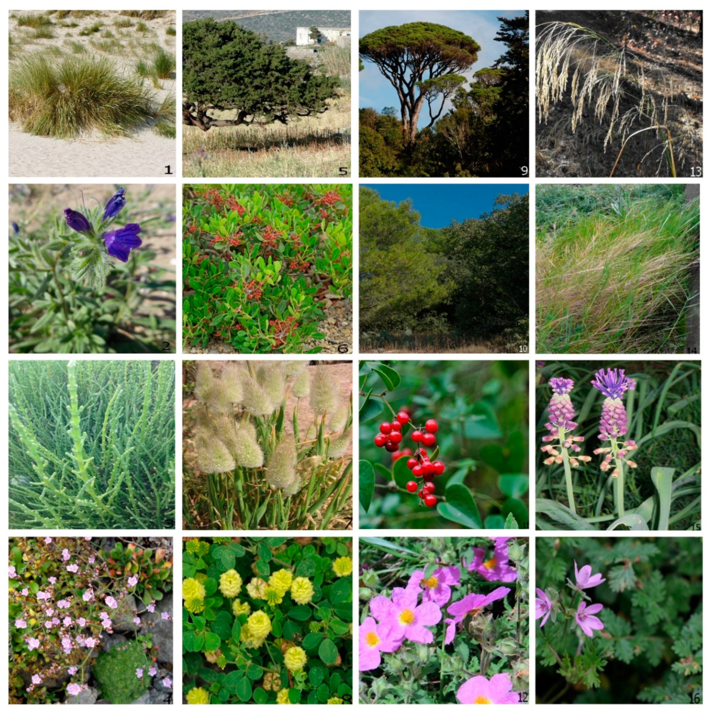
Figure 1. Schinias study area at the northeastern part of Attica, Greece. The grey line together with the sea front circumscribes the study area. The black line with a west–east direction indicates the road leading to the base of the Kynosoura Peninsula. The numbers show the habitats revealed in this study on the basis of their insect content.
Forests 14 00392 g001
Figure 2. Diagram showing the number of species in each out of 18 functional roles. The numbered strands of the highest bar corresponding to the functional role of predators correspond to each of the seven habitat types. The lateral text box explains the symbols of the functional roles.
Forests 14 00392 g002
Figure 3. Sketch showing the Holocene evolution of the Schinias pinewood and marsh. The transverse cut corresponds to the straight red line in the previous panel. Four stages span the time from prehistory (stage 1) to the present (stage 4).
Forests 14 00392 g003
Figure 4. Mean specificity of the seven habitat types. Columns marked with different letters denote specificities that are significantly different (p < 0.05). Error bars are 1 sem.
Forests 14 00392 g004
Figure 5. Diagram showing the absolute values of the three components α, β spatial, β temporal of biodiversity and the height of the bar corresponds to total (γ) biodiversity. Different letters within bars represent bar segments that cannot be declared different at the p = 0.05 level across all habitat types. Three triplets were used for the segments, namely [a,b,c], [x,y,z], and [p,q,r].
Forests 14 00392 g005
Figure 6. Diagram of V-statistic of all 63 plots. All nine plots of each habitat type are within each ellipsis that corresponds and circumscribes each habitat. The nine symbols, whether empty or filled or of any shape within the same ellipsis, correspond to plots of the same vegetation type. All plots in one ellipsis are of the same color.
Forests 14 00392 g006
Figure 7. Stacked bar diagram showing the proportion of total (γ) partitioned to α, βspatial, βtemporal diversity. The lower part of each column corresponds to the mean bimonthly α diversity.
Forests 14 00392 g007
Figure 8. Four-variable diagram of the three impact types and the number of indicator insect species of the seven habitats. The triangle configuration has each side numbered as percentage. Spikes from each habitat point are drawn to facilitate inspection.
Forests 14 00392 g008
Table 1. Habitats and the major plant species grown in the Schinias coastal pinewood area. Photos of these plants are in Figure A2.
NameDominant and Subdominant Plants
H1P.halepensis, Pistacia lentiscus L., Juniperus phoenicea L., Anthylis hermaniae L.
H2P. halepensis Mill, Poaceae, Cistus sp., Papilionaceae, Brassicaceae
H3P. pinea L., Pa. Lentiscus, Juniperus oxycedrus subsp. macrocarpa (Sm.) Neilr., A. hermaniae
H4P. pinea, Poaceae, Pa. lentiscus, Quercus coccifera L., Asparagus aphyllus L., Cistus sp.
H5Typha angustifolia L., Plantago coronopus L., T. hampeana, J. acutus L., Elymus farctus (Viv.) Runemark ex Melderis
H6J. subulatus Forssk., Phragmites australis (Cav.) Trin. ex Steud.
H7T. hampeana, Cakile maritima Scop.
Table 2. Metrics used in nestedness and co-occurrence analysis.
MetricObserved ValueZP
T31.04 3−1.34Ns
NODF 162.81.05Ns
WNODF 228.140.38Ns
C-score 4141.344.65 × 10−4
CU 51,375,256319.38<0.01
1 is the acronym of the nestedness measure of decreasing fill for presence/absence data; 2 is the acronym of the weighted nestedness measure of decreasing fill for abundance data; 3 with 52.3% matrix fill; 4 is the acronym of checkerboard units; 5 it is a statistic that determines the randomness of the distribution of two or more species in a set of data.
Disclaimer/Publisher’s Note: The statements, opinions and data contained in all publications are solely those of the individual author(s) and contributor(s) and not of MDPI and/or the editor(s). MDPI and/or the editor(s) disclaim responsibility for any injury to people or property resulting from any ideas, methods, instructions or products referred to in the content.

