Determining Asymptotic Stability and Robustness of Networked Systems

Abstract

This paper is motivated by the notion that coupling systems allows for mitigating the failure of individual ones. We present a novel approach to determining asymptotic stability and robustness of a network consisting of coupled dynamical systems, where individual system dynamics are represented through polynomial or rational functions. The analysis relies on a local analysis; thus, making it computationally implementable. We present an efficient computational method that relies on semidefinite programming. Importantly, for cases where multiple equilibrium points exist, we show how to determine regions around an asymptotically stable equilibrium point that bounds solutions. These regions increase when systems are coupled as we observe when applying the presented analysis framework to a mathematical model of a continuous stirred tank reactor. Importantly, the presented work has implications to other fields as well.

1. Introduction

We are currently experiencing rapid digitalisation and automatisation in industry and society, which are culminating in the notions of smart factories, smart cities, the industry of things, and the internet of things. This makes networked systems and their control increasingly gaining in importance [1,2,3]. Significantly, networked sensor and actuator systems are also already pervasive in many traditional industries, for instance, the petroleum industry [4]. Additionally, networks of coupled dynamical systems appear also in other areas such as modelling of the heart [5] and of flocking behaviour [2]. An important question in network science, which links the dynamics of individual nodes with the emergent properties of macroscopic networks [6], is how much failure a networked system can tolerate. From the perspective of control engineering, a networked system can be viewed as a system of coupled dynamical systems and the question can be formulated in terms of asymptotic stability, the ability to return to a steady state, and robustness, the ability to withstand failures and perturbations.

In recent years, tools have been developed to determine whether a given complex network, consisting of connected systems, is robustly controllable, that is, whether any desired state can be reached from any initial state for almost all values of network edge-weights. For linear systems, conditions based on structural controllability, which identifies the minimal number of inputs or controllable nodes for system controllability of a complex network, were developed in [7,8]. For nonlinear systems, an equivalent approach based on feedback vertex set control, which is an attractor-based control method and requires thorough system knowledge, has been presented in [9]. However, these works and the majority of related ones rather consider systems that do not represent dynamical processes, as highlighted in [10], where the authors studied networks with node behaviour, which better represents dynamical behaviour that is typical for many systems, and examined how this influences the properties of the network. Using their analysis framework, they generated more realistic, albeit still simplified, results.

In this work, we provide certificates for asymptotic stability and robustness of complex networked systems consisting of coupled realistic system models through local analysis, which makes the approach computationally implementable and does not require simplifying the individual node dynamics. For this, we use so-called barrier certificates [11] and semidefinite programming [12,13]. For dynamical systems, the authors of [11] introduced a safety verification method that relies on state functions termed barrier certificates. Such functions form contour levels and, thus, create different regions in the state space. For a given set of initial conditions, the zero-level set of a barrier certificate bounds corresponding system trajectories and, by doing so, separates safe from unsafe regions. This means that one obtains certificates or proofs of system safety without the need to compute system behaviour explicitly. The use of different types of barrier certificates is popular in fields as diverse as biological model-testing, using the noise inherent in such systems [14], and avoiding collisions in multi-robot systems [15]. For our results, barrier certificates provide means to assess the set of initial conditions that will converge towards a desired operating point.

Related work has been presented in [16], where global stability for coupled differential equations was investigated assuming a Lyapunov function [17] of the form $V\left(x\right)=x-x^{*}lnx$, where $x^{*}$ is a positive equilibrium point. This approach was later extended to coupled systems with time-varying coupling [18]. As a novelty, the approach presented in this paper provides not only means to search for a Lyapunov function that guarantees asymptotic stability of the coupled system, for systems with multiple equilibria, it also uses Lyapunov theory to provide regions of attraction, even when model parameters are uncertain (robustness).

In many areas of research, realistic dynamical system models are based on ordinary differential equations described by polynomial or rational functions. Assuming such models, in Section 2.1 and Section 2.2, we provide results on testing for asymptotic stability and robustness of a networked system through a local analysis of the system. Locality makes the analysis feasible and allows for its computational implementation, as we show in Section 2.3. Meanwhile, for simplicity, we first assume all-to-all coupling, in Section 2.4, we extend the results to arbitrary coupling topologies. Section 3 provides an application to process engineering, where we analyse the stability and robustness of a high biomass concentration steady state for connected continuous stirred tank reactors. Finally, we discuss our results and conclude the paper in Section 4.

2. Asymptotic Stability of Coupled Dynamical Systems

In this paper, we consider bidirectional coupling only. Furthermore, let us consider N dynamical systems that are linearly all-to-all coupled. Then, we represent the i-th system through

$${\dot{x}}_i=f_i\left(x_i\right)+\sum _{j=1}^{N}kD(x_j-x_i),$$

(1)

where $f_i:{\mathbb{R}}^n\to {\mathbb{R}}^n$ describes the system’s dynamics for all i, $i\in \{1,2,\dots ,N\}$, $x={[x_1\cdots x_N]}^{\mathrm{T}}$, $x_i\left(t\right)\in {\mathbb{R}}^n$, and $D\in {\mathbb{R}}^{n\times n}$. Vector x is the state vector. Matrix D is the matrix that denotes the variables that are used in the coupling; that is, $D_{(k,l)}\ne 0$ if and only if states $x_{i_{\left(k\right)}}$ and $x_{j_{\left(l\right)}}$ are coupled, for all $i,j$ and $i\ne j$. Positive constant k corresponds to the coupling strength. Next, we provide results on asymptotic stability of the coupled system based on Lyapunov theory.

2.1. Unique Equilibrium Point

First, let us assume that the networked system described by N coupled systems given by Equation (1) has a unique global equilibrium point. Without loss of generality, let it be the origin; otherwise, the equilibrium point can be shifted to the origin through a change of variables. Moreover, we assume that ${\dot{x}}_1=f_1\left(x_1\right)$ is asymptotically stable. We do this, because, without proof, the networked system can only be asymptotically stable if at least one individual system is asymptotically stable, whose state we denote by $x_1$, without loss of generality. If we consider all other systems to be similar to this system but to possess a certain amount of bounded parameter uncertainty then condition (4), which we derive in the following, guarantees that the coupled system is asymptotically stable. This allows us to assess the robustness of a networked system.

Now, consider the following Lyapunov function,

$$V\left(x\right)=\sum _{i=2}^N\left(\frac{1}{2}\frac{1}{N-1}{x}_1^{\mathrm{T}}M{x}_1+\overline{V}\left(X_i\right)\right)=\sum _{i=2}^N\tilde{V}(x_1,X_i),$$

(2)

where $X_i=x_i-x_1$, $M=M^{\mathrm{T}}\succ 0$, and $\tilde{V}(x_1,X_i)\ge 0$. Moreover, $\tilde{V}(x_1,X_i)>0$ if neither $x_1=0$ nor $X_i=0$, for all i. Thus, $V\left(x\right)>0$ unless $x=0$. Then,

$$\begin{array}{ccc}\hfill \dot{V}\left(x\right)& =& \sum _{i=2}^N\left(\frac{1}{2}\frac{1}{N-1}\left({\dot{x}}_1^{\mathrm{T}}M{x}_1+x_1^{\mathrm{T}}M{\dot{x}}_1\right)+\dot{\overline{V}}\left(X_i\right)\right)=\sum _{i=2}^N\left(\frac{1}{N-1}{x}_1^{\mathrm{T}}M{\dot{x}}_1+\dot{\overline{V}}\left(X_i\right)\right)\hfill \\ & =& \sum _{i=2}^N\left(\frac{1}{N-1}{x}_1^{\mathrm{T}}M\left(f_1\left(x_1\right)+kD\sum _{j=2}^N{X}_j\right)+\frac{\partial \overline{V}\left(X_i\right)}{\partial X_i}(f_i\left(x_i\right)-f_1\left(x_1\right)-kND{X}_i)\right)\hfill \\ & =& \sum _{i=2}^N\left(\frac{1}{N-1}{x}_1^{\mathrm{T}}M{f}_1\left(x_1\right)+x_1^{\mathrm{T}}kMD{X}_i+\frac{\partial \overline{V}\left(X_i\right)}{\partial X_i}(f_i\left(x_i\right)-f_1\left(x_1\right)-kND{X}_i)\right).\hfill \end{array}$$

(3)

The second equality in the first line of Equation (3) follows from the symmetry of M. Thus, if

$$\frac{1}{N-1}{x}_1^{\mathrm{T}}M{f}_1\left(x_1\right)+x_1^{\mathrm{T}}kMD{X}_i+\frac{\partial \overline{V}\left(X_i\right)}{\partial X_i}(f_i\left(x_i\right)-f_1\left(x_1\right)-kND{X}_i)<0$$

(4)

holds for all i unless $x_1=0$ and $X_i=0$ for all i, and, thus, unless $x=0$, then $\dot{V}<0$ unless $x=0$, which guarantees asymptotic stability of the coupled system. Finally, for all i, we consider the differences in function $f_i\left(x_i\right)$ to depend on r real parameters that are uncertain but whose values are bounded. Let these parameters be elements of vector $q\in \mathcal{Q}\subset {\mathbb{R}}^r$. Then, we can rewrite condition (4) by letting $g(q_1,x_1)\equiv f_1\left(x_1\right)$ and $g(q_i,x_i)\equiv f_i\left(x_i\right)$. In this case, if condition (4) holds, for all $x_1,x_i\in {\mathbb{R}}^n$ and all $q_1,q_i\in \mathcal{Q}$, then asymptotic stability of the coupled system is guaranteed.

2.2. Multiple Equilibrium Points

Second, if the networked system possesses multiple equilibrium points, then inequality (4) can only hold in a certain region of the state space. In order to estimate this region, we assume, again, that the equilibrium point, whose stability properties we wish to investigate, is the origin. Then, if inequality (4) holds for $\tilde{V}(x_1,X_i)<c$, $c\in \mathbb{R}$, $c>0$, and all i then $\tilde{V}(x_1,X_i)$ decreases with time for all i and, thus, so does $V\left(x\right)$, which means that the origin is asymptotically stable in the region bounded by $V\left(x\right)=c$. As we will show in Section 3, in addition to above robustness analysis, determining this region allows us to assess how far a system can deviate from a particular steady state and still remain attracted by the latter.

2.3. Computational Implementation

2.3.1. Coupled Linear Systems

Consider N coupled linear dynamical systems of the form ${\dot{x}}_1=Ax$ and ${\dot{x}}_i=Bx$ for all $i>1$, where $A,B\in {\mathbb{R}}^{n\times n}$, matrix A is stable, and matrix B is a matrix that is similar to A, however, with some uncertain but bounded entries. Then, for $\overline{V}\left(X_i\right)=X_i^{\mathrm{T}}P{X}_i$, where $P=P^{\mathrm{T}}\succ 0$, inequality (4) becomes

$$\begin{array}{ccc}\hfill & & x_1^{\mathrm{T}}\left(M\left(\frac{1}{N-1}A-kD\right)+P(A-kND)\right)x_1\hfill \\ & & +x_1^{\mathrm{T}}\left(kMD+P(kND-B)\right)x_i+x_i^{\mathrm{T}}P(kND-A)x_1+x_i^{\mathrm{T}}P(B-kND)x_i<0.\hfill \end{array}$$

(5)

Given k, the problem of determining matrices M and P such that Equation (2) and inequality (5) hold can be cast as a semidefinite programme of the following form

$$\begin{array}{ccc}\hfill \mathrm{given}& & A,B,D,N,k\hfill \\ \hfill \mathrm{search}\mathrm{for}& & M,P\hfill \\ \hfill \mathrm{subject}\mathrm{to}& & M=M^{\mathrm{T}}\succ 0,P=P^{\mathrm{T}}\succ 0,\left(5\right).\hfill \end{array}$$

(6)

Problem (6) is a classic case of linear matrix inequalities [19] that can be solved efficiently using, for example, YALMIP, a free, third-party MATLAB toolbox [20], which can handle bounded uncertainties in B [21] to obtain robustness certificates.

2.3.2. Coupled Nonlinear Systems

For nonlinear systems, we investigate those ones whose dynamics are modelled using polynomial or rational functions. Consider the real-valued polynomial function $F\left(x\right)$ of degree $2d$, $x\in {\mathbb{R}}^n$. Testing for non-negativity is NP-hard [22]. However, a sufficient condition for $F\left(x\right)$ to be nonnegative is that it can be decomposed into a sum of squares (SOS) [23]:

$$F\left(x\right)=\sum _i{f}_i^2\left(x\right)\ge 0,$$

(7)

where $f_i$ are polynomial functions. Now, $F\left(x\right)$ is a SOS if and only if there exists a positive semidefinite matrix R and

$$F\left(x\right)=\sum _i{f}_i^2\left(x\right)={\chi }^{\mathrm{T}}R\chi ,\chi =[1,x_{\left(1\right)},x_{\left(2\right)},\dots ,x_{\left(n\right)},x_{\left(1\right)}{x}_{\left(2\right)},\dots ,x_{\left(n\right)}^d].$$

(8)

The entries of vector $\chi$ consist of all monomial combinations of the elements of vector x up to degree d (including $x_{\left(i\right)}^0=1$) and, thus, its length is $\ell =\left(\genfrac{}{}{0pt}{}{n+d}{d}\right)$. Note that R is not necessarily unique. However, Equation (8) poses certain constraints on R of the form trace $\left(A_{j}R\right)=c_j$, where $A_j$ and $c_j$ are appropriate matrices and constants respectively. As an illustration, in the following, we reproduce Example 3.5 of [23].

Consider the following polynomial function, where $z_1=x_1^2$, $z_2=x_2^2$, $z_3=x_1{x}_2$:

$$\begin{array}{ccc}\hfill F\left(x\right)& =& 2x_1^4+2x_1^3{x}_2-x_1^2{x}_2^2+5x_2^4\hfill \\ & =& {\left[\begin{array}{c}{x}_1^2\\ x_2^2\\ x_1{x}_2\end{array}\right]}^{\mathrm{T}}\left[\begin{array}{ccc}{q}_{11}& q_{12}& q_{13}\\ q_{12}& q_{22}& q_{23}\\ q_{13}& q_{23}& q_{33}\end{array}\right]\left[\begin{array}{c}{x}_1^2\\ x_2^2\\ x_1{x}_2\end{array}\right]\hfill \\ & =& q_{11}{x}_1^4+q_{22}{x}_2^4+(q_{33}+2q_{12})x_1^2{x}_2^2+2q_{13}{x}_1^3{x}_2+2q_{23}{x}_1{x}_2^3.\hfill \end{array}$$

This leads to the following set of linear equalities:

$$q_{11}=2,q_{22}=5,q_{33}+2q_{12}=-1,2q_{13}=2,2q_{23}=0.$$

Thus, $j=1,\dots ,5$, and, for example, $c_1=2$, $c_3=-1$,

$$A_1=\left[\begin{array}{ccc}1& 0& 0\\ 0& 0& 0\\ 0& 0& 0\end{array}\right],\mathrm{and}{A}_3=\left[\begin{array}{ccc}0& 1& 0\\ 1& 0& 0\\ 0& 0& 1\end{array}\right].$$

In general, in order to find R, we solve the optimisation problem associated with the following semidefinite program:

$$\begin{array}{ccc}\hfill \mathrm{minimise}& & \mathrm{trace}\left(A_{0}R\right)\hfill \\ \hfill \mathrm{subject}\mathrm{to}& & \mathrm{trace}\left(A_{j}R\right)=c_j,j=1,\dots ,m\hfill \\ & & R=R^{\mathrm{T}}⪰0.\hfill \end{array}$$

(9)

In this paper, to solve SOS programmes, we use SOSTOOLS [24], a free, third-party MATLAB toolbox. For instance, the problem of determining Lyapunov function $\tilde{V}(x_1,X_i)$, given by Equation (2), such that (4) holds can be cast as follows

$$\begin{array}{ccc}\hfill \mathrm{given}& & f_1\left(x_1\right),f_i\left(x_i\right),D,N,k\hfill \\ \hfill \mathrm{search}\mathrm{for}& & \tilde{V}(x_1,X_i)\hfill \\ \hfill \mathrm{subject}\mathrm{to}& & -\epsilon (x_1^{\mathrm{T}}{x}_1+x_i^{\mathrm{T}}{x}_i)+\tilde{V}(x_1,X_i)\mathrm{is}\mathrm{SOS},\hfill \\ & & -\epsilon (x_1^{\mathrm{T}}{x}_1+x_i^{\mathrm{T}}{x}_i)-\dot{\tilde{V}}(x_1,X_i)\mathrm{is}\mathrm{SOS},0<\epsilon \ll 1.\hfill \end{array}$$

(10)

Here, some additional remarks:

• Consider a rational function $F\left(x\right)$, $F\left(x\right)=\frac{f\left(x\right)}{g\left(x\right)}$, where $f\left(x\right)$ and $g\left(x\right)$ are polynomial functions. Then, $F\left(x\right)\ge 0$ if (9) is feasible with ${\chi }^{\mathrm{T}}R\chi =F\left(x\right)g^2\left(x\right)$ or with ${\chi }^{\mathrm{T}}R\chi =F\left(x\right)g\left(x\right)$ if $g\left(x\right)>0$.
• If

  $$\begin{array}{c}\hfill F\left(x\right)+p\left(x\right)h\left(x\right)=\sum _i{g}_i^2\left(x\right)\ge 0,p\left(x\right)\ge 0,\\ \hfill h\left(x\right)=\left\{\begin{array}{c}\le 0\mathrm{if}{a}_i\le x_{\left(i\right)}\le b_i\forall i\hfill \\ >0\mathrm{otherwise}\hfill \end{array}\right.,\end{array}$$

  then $F\left(x\right)\ge 0$ if $a_i\le x_{\left(i\right)}\le b_i$ for all i, where $a_i,b_i$ are constants. This can be used to show that $F\left(x\right)$ is nonnegative in a specific region of the state and/or parameter space.
• Finally, the computational time necessary to solve SOS decomposition problems scales badly with the size of the problem, as the length of vector is $\ell =\left(\genfrac{}{}{0pt}{}{n+d}{d}\right)$.

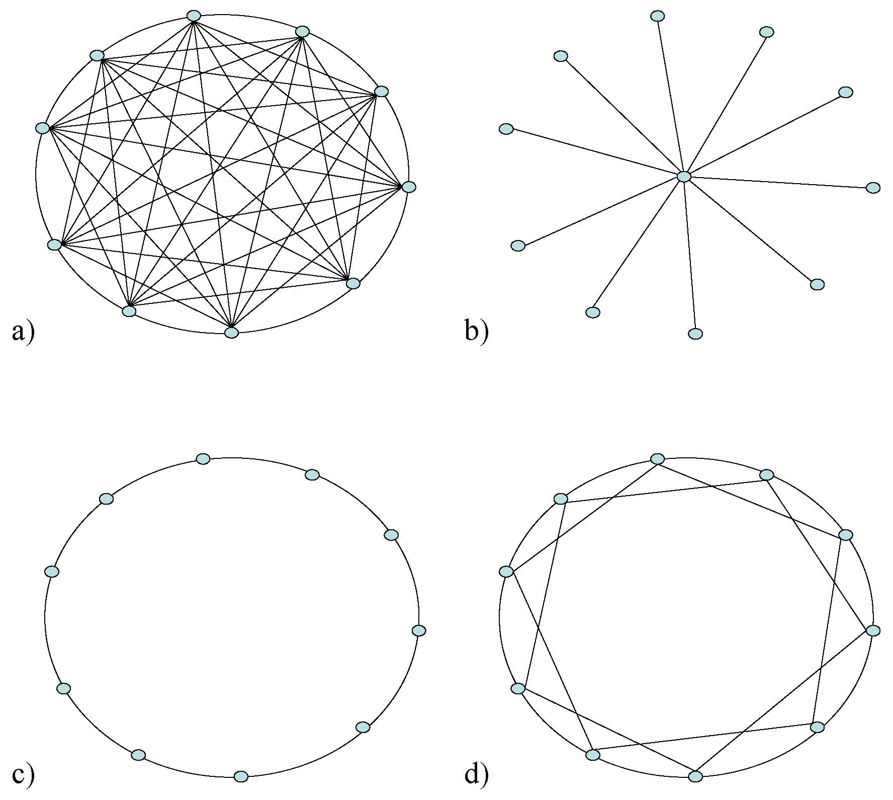
2.4. Different Coupling Configurations

The presented results can be extended to any symmetric linear coupling topology with corresponding Laplacian matrix $-C$ by letting $\overline{V}\left(X_i\right)=X_i^{\mathrm{T}}P{X}_i$, for all i, in Equation (2), where $P=P^{\mathrm{T}}\succ 0$. To show this, first, we define the Laplacian matrix of the completely connected graph given by $-U\in {\mathbb{R}}^{N\times N}$ through

$$-U=N{I}_N-E⪯0,E=e{e}^{\mathrm{T}},e={[1\dots 1]}^{\mathrm{T}}.$$

(11)

Note that the eigenvalues of $-U$ are ${\lambda }_1=0$ and ${\lambda }_i=N$ for all $i>1.$ Then, the following lemma establishes a relation between C and U.

Lemma 1.

Let $U,C\in {\mathbb{R}}^{N\times N}$, where $-U$ is the Laplacian matrix of the completely connected graph defined in Equation (11) and $-C$ is a symmetric Laplacian matrix of rank $(N-1)$. Then, for all $y\in {\mathbb{R}}^N$,

$$y^{\mathrm{T}}Cy\le \frac{{\lambda }_{min}(-C)}{N}{y}^{\mathrm{T}}Uy,$$

(12)

where ${\lambda }_{min}(-C)$ denotes the smallest positive eigenvalue of the matrix $-C$.

Proof. 

First, note that $C_{(i,j\ne i)}\ge 0$. Now, $UE=0$ and $CE=0$. Hence, $UU=-NU$ and $CU=-NC$. By the Spectral Theorem, there exists a unitary matrix S such that $S^{-1}=S^{\mathrm{T}}$ and $-SC{S}^{\mathrm{T}}={\Lambda }_{-C}$, where ${\Lambda }_{-C}$ is the diagonal matrix containing the eigenvalues of $-C$ and, without loss of generality, its first entry is 0. Moreover,

$$SCU{S}^{\mathrm{T}}=SC{S}^{\mathrm{T}}SU{S}^{\mathrm{T}}=-SC{S}^{\mathrm{T}}N=SC{S}^{\mathrm{T}}{\Lambda }_U$$

implies that $SU{S}^{\mathrm{T}}={\Lambda }_U$, where ${\Lambda }_U$ is the diagonal matrix containing the eigenvalues of U, which are $-N$ but for the first one, which is 0. Now, for all $y\in {\mathbb{R}}^N$ and ${\Lambda }_C$ being the diagonal matrix containing the eigenvalues of C,

$$y^{\mathrm{T}}Cy=y^{\mathrm{T}}{S}^{\mathrm{T}}{\Lambda }_{C}Sy=v^{\mathrm{T}}{\Lambda }_{C}v\le \frac{{\lambda }_{min}(-C)}{N}{v}^{\mathrm{T}}{\Lambda }_{U}v=\frac{{\lambda }_{min}(-C)}{N}{y}^{\mathrm{T}}{S}^{\mathrm{T}}{\Lambda }_{U}Sy=\frac{{\lambda }_{min}(-C)}{N}{y}^{\mathrm{T}}Uy,$$

which completes the proof. □

Consider, again, difference $X_i\equiv x_i-x_1$, where $X_i\in {\mathbb{R}}^n$ and $X_1=0$ [25]. Let matrix $F\in {\mathbb{R}}^{N\times N}$ be defined as follows,

$$F=\left[\begin{array}{ccccc}0& 0& 0& \dots & 0\\ -1& 1& 0& \dots & 0\\ -1& 0& 1& \dots & 0\\ ⋮& ⋮& ⋮& \ddots & ⋮\\ -1& 0& 0& \dots & 1\end{array}\right].$$

(13)

Then,

$$X=(F\otimes I_n)x,X,x\in {\mathbb{R}}^{Nn},$$

(14)

and

$$\dot{X}=(F\otimes I_n)\dot{x}.$$

(15)

Moreover, note that for symmetric coupling determined by Laplacian matrix $-C$, $C=CF$ and $FU=-NF$. Let $\tilde{f}\left(x\right)={[f_1\left(x_1\right)\dots f_N\left(x_N\right)]}^{\mathrm{T}}$. Then,

$$\begin{array}{ccc}\hfill \sum _{j=2}^N\dot{\overline{V}}(X_i)& =& X^{\mathrm{T}}(I_N\otimes P)\dot{X}=X^{\mathrm{T}}(F\otimes P)\dot{x}\hfill \\ & =& X^{\mathrm{T}}(F\otimes P)(\tilde{f}(x)+k(C\otimes D)x)\hfill \\ & =& X^{\mathrm{T}}(F\otimes P)(\tilde{f}(x)+k(CF\otimes D)x)\hfill \\ & =& X^{\mathrm{T}}(F\otimes P)(\tilde{f}(x)+k(C\otimes D)X)\hfill \\ & \le & X^{\mathrm{T}}(F\otimes P)(\tilde{f}(x)+\alpha k(U\otimes D)X)\hfill \\ & =& \sum _{i=2}^N{X}_i^{\mathrm{T}}P(f_i(x_i)-f_1(x_1))+\alpha k{X}^{\mathrm{T}}(FU\otimes PD)X\hfill \\ & =& \sum _{i=2}^N{X}_i^{\mathrm{T}}P(f_i(x_i)-f_1(x_1))-\alpha Nk{X}^{\mathrm{T}}(F\otimes PD)X\hfill \\ & =& \sum _{i=2}^N{X}_i^{\mathrm{T}}P(f_i(x_i)-f_1(x_1)-\alpha kND{X}_i),\hfill \end{array}$$

where the inequality follows from Lemma 1, $\alpha N={\lambda }_{min}(-{(FC)}_{\mathrm{gL}})$, and ${(FC)}_{\mathrm{gL}}$ is the matrix obtained by deleting the first row and the first column of $FC$. It is the so-called grounded Laplacian [26,27], where the deleted row and deleted column correspond to the grounded variable—in our case it is $x_1$. A grounded Laplacian matrix is a principal sub-matrix of the Laplacian matrix. The fact that, for square matrices $A,B$, $\mathrm{eig}(AB)=\mathrm{eig}(BA)$, has been proven in [28] and, thus, $\mathrm{eig}(FC)=\mathrm{eig}(CF)=\mathrm{eig}(C)$. Since the first row of matrix $FC$ is zero, it follows that ${\lambda }_{min}(-{(FC)}_{\mathrm{gL}})={\lambda }_{min}(-C)$. For illustration, we provide examples of ${\lambda }_{min}(-C)$ of different unweighted coupling configurations.

(a)

All-to-all coupling ($C=U$): ${\lambda }_{min}(-C)=N$.

(b)

Star-configuration: ${\lambda }_{min}(-C)=1$.

(c)

Ring of diffusively coupled systems: ${\lambda }_{min}(-C)=4{sin}^2\frac{\pi }{N}$.

(d)

Ring of $2k$-nearest neighbour coupled systems [29]: ${\lambda }_{min}(-C)\simeq 2{\pi }^{2}k(k+1)(2k+1)/3N^2$ if $k\ll N$.

The different coupling configurations are illustrated in Figure 1.

Figure 1. Four different coupling configurations. Here, $N=10$ in (a,c,d), $N=11$ in (b), and $k=2$ in (d).

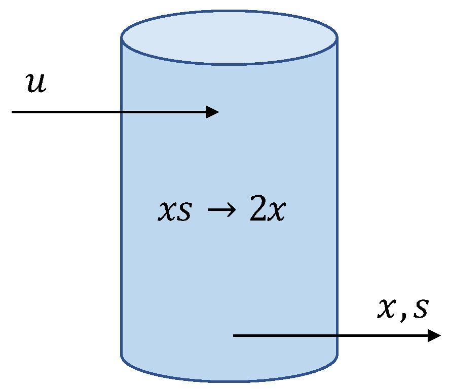
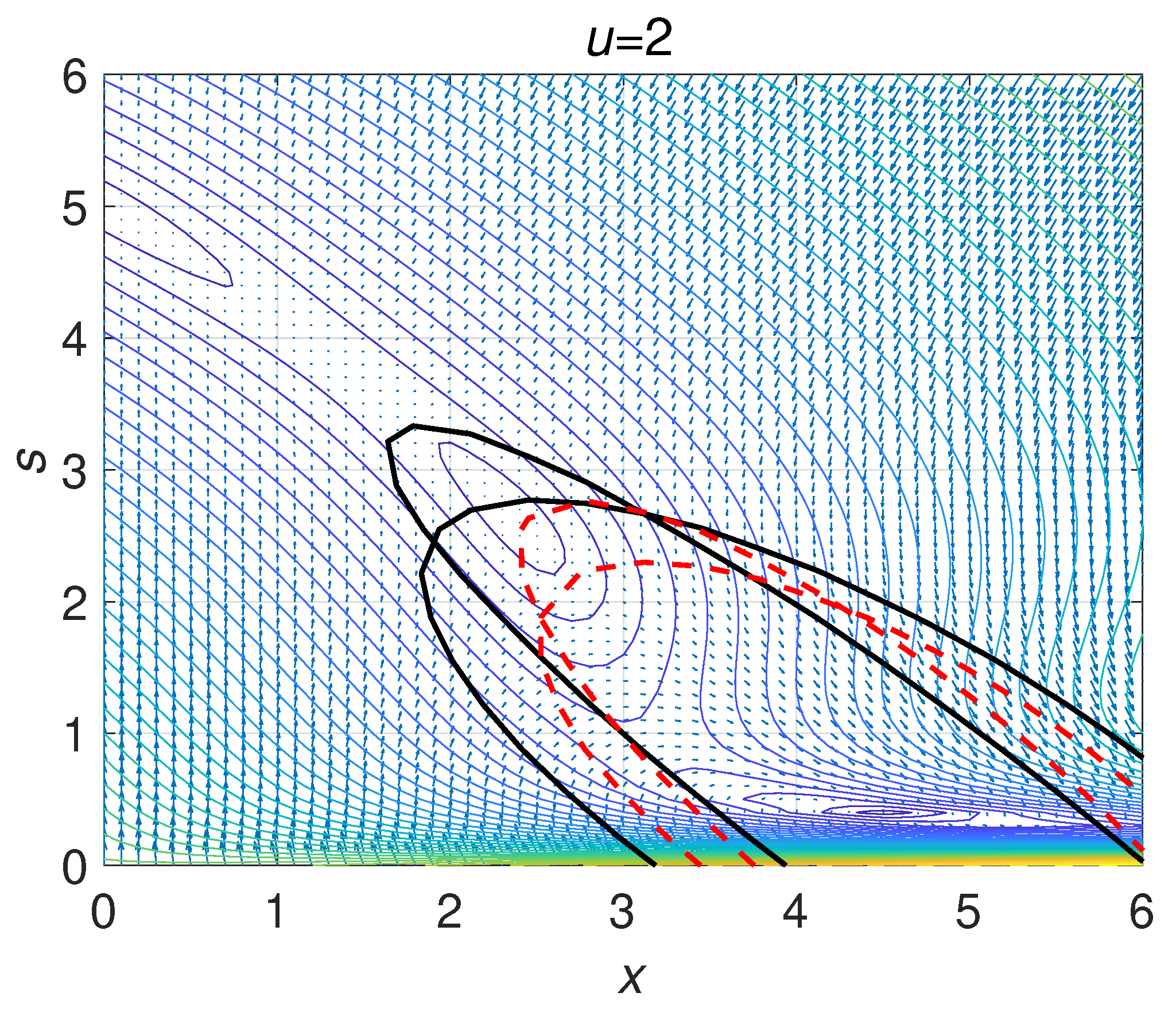
3. Coupled Continuous Stirred Tank Reactors

Consider a continuous stirred tank reactor for biomass production held at a constant temperature [30]. Concentrations of feed or substrate are denoted by s and those of the product by x (Figure 2). The reaction describing the inflow and outflow of substrate and outflow/harvesting of product is given by $x\to \varnothing \rightleftarrows s$. The reaction describing the growth of product by consuming substrate is given by $xs\stackrel{k}{\to }2x$, where reaction constant k is described below.

Figure 2. Schematic view of a continuous stirred tank reactor.

The corresponding mathematical model based on ordinary differential equations is given by

$$\begin{array}{ccc}\hfill \dot{x}& =& \frac{2xs}{{(s+1)}^2}-0.4x,\hfill \\ \hfill \dot{s}& =& u-\frac{2xs}{{(s+1)}^2}-0.4s,\hfill \end{array}$$

(16)

where we denote the input rate of substrate by u. Moreover, we assume an outflow rate of $0.4$ (unitless) and a reaction rate of $kxs$, where $k=\frac{2}{{(s+1)}^2}$ implies inhibition for high concentrations of substrate (poisoning). We denote equilibrium points by $x^{*}$ and $s^{*}$. Figure 3 shows the phase plot with the vector field for $u=2$, which depicts the behaviour of the system, determined through the direction set by the vector arrows, in dependence of its state. For $u=2$, there are three equilibrium points, which are clearly visible. The equilibrium point that corresponds to higher concentrations of product is given by $x^{*}=4.618$ and $s^{*}=0.382$. Note that the system described by Equation (16) is a nonnegative system such that for nonnegative initial conditions, solutions remain in the nonnegative orthant [31]. To obtain a set that bounds solutions, we let $\overline{x}=x+x^{*}$ and $\overline{s}=s+s^{*}$, first, solve the following problem

$$\begin{array}{ccc}\hfill \mathrm{given}& & \mathrm{Equation}\left(16\right),u=2,\beta \in \mathbb{R}\hfill \\ \hfill \mathrm{search}\mathrm{for}& & M\hfill \\ \hfill \mathrm{subject}\mathrm{to}& & p_1(\overline{x},\overline{s}),p_2(\overline{x},\overline{s}),p_3(\overline{x},\overline{s})\mathrm{are}\mathrm{SOS}\mathrm{functions}\mathrm{of}\mathrm{degree}4,\hfill \\ & & -0.001({\overline{x}}^2+{\overline{s}}^2)+V_1\mathrm{is}\mathrm{SOS},V_1=\frac{1}{2}{\left[\begin{array}{c}\overline{x}\\ \overline{s}\end{array}\right]}^{\mathrm{T}}M\left[\begin{array}{c}\overline{x}\\ \overline{s}\end{array}\right],\hfill \\ & & -0.001({\overline{x}}^2+{\overline{s}}^2)-{\dot{V}}_1·{(s+1)}^2+p_1(\overline{x},\overline{s})({\overline{x}}^2+{\overline{s}}^2-\beta )-p_2(\overline{x},\overline{s})x-p_3(\overline{x},\overline{s})s\mathrm{is}\mathrm{SOS},\hfill \end{array}$$

(17)

for different values of $\beta$, and, then, solve

$$\begin{array}{ccc}\hfill \mathrm{given}& & V_1\hfill \\ \hfill \mathrm{minimise}& & -\gamma ,\gamma \in \mathbb{R}\hfill \\ \hfill \mathrm{subject}\mathrm{to}& & p_1(\overline{x},\overline{s}),p_2(\overline{x},\overline{s}),p_3(\overline{x},\overline{s})\mathrm{are}\mathrm{SOS}\mathrm{functions}\mathrm{of}\mathrm{degree}2,\hfill \\ & & V_1-\gamma -p_1(\overline{x},\overline{s})({\overline{x}}^2+{\overline{s}}^2-\beta )-p_2(\overline{x},\overline{s})x-p_3(\overline{x},\overline{s})s\mathrm{is}\mathrm{SOS}.\hfill \end{array}$$

(18)

Figure 3. Phase plot with vector field and corresponding contour lines, for the system described by Equation (16), and regions that bound solutions (red dashed lines). For coupling of a few such systems as in Equation (1) and for $N>1$, solutions are bounded by the black solid lines.

The boundary of the set is given by $V_1=\gamma$. Figure 3 depicts the sets defined by $\beta =7$ and $\beta =9.95$. Their boundaries are given by the dashed red lines. For $\beta >9.95$, programme (17) is infeasible and remains so even after increasing the degree of polynomials $p_1$, $p_2$, and $p_3$. Note that outside the regions, whose boundaries are given by the dashed red line in Figure 3, one might risk washout or depletion of product by being attracted to the equilibrium point given by $x^{*}=0$ and $s^{*}=5$.

Now, by interconnecting reactors as in Equation (1), we can mitigate the danger of washout that might result, for example, from disturbances. Note that in our modelling, we assume full control over all flow rates, that is, in all inlets, where we let $u=2$, and between all reactors, where $k=5$. For $N>1$, we solve the following problem, which is analogous to problem (17),

$$\begin{array}{ccc}\hfill \mathrm{given}& & \mathrm{Equation}\left(16\right),\mathrm{Equation}\left(1\right),u=2,k=5,D=I_2,N>1,\beta \in \mathbb{R}\hfill \\ \hfill \mathrm{search}\mathrm{for}& & \tilde{V}({\overline{x}}_1,{\overline{s}}_1,{\overline{x}}_i,{\overline{s}}_i)\hfill \\ \hfill \mathrm{subject}\mathrm{to}& & p_j({\overline{x}}_1,{\overline{s}}_1,{\overline{x}}_i,{\overline{s}}_i)\mathrm{are}\mathrm{SOS}\mathrm{functions}\mathrm{of}\mathrm{degree}4,j\in \{1,\dots ,5\},\hfill \\ & & \tilde{V}=\frac{1}{2}\frac{1}{N-1}{x}_1^{\mathrm{T}}M{x}_1+\overline{V}\left(X_i\right)\mathrm{is}\mathrm{a}\mathrm{SOS}\mathrm{function}\mathrm{of}\mathrm{degree}2,\hfill \\ & & -0.001({\overline{x}}_1^2+{\overline{s}}_1^2+{\overline{x}}_i^2+{\overline{s}}_i^2)+\tilde{V}\mathrm{is}\mathrm{SOS},\hfill \\ & & -0.001({\overline{x}}_1^2+{\overline{s}}_1^2+{\overline{x}}_i^2+{\overline{s}}_i^2)-\dot{\tilde{V}}·{({\overline{s}}_1+1)}^2{({\overline{s}}_i+1)}^2\hfill \\ & & +p_1·({\overline{x}}_1^2+{\overline{s}}_1^2+{\overline{x}}_i^2+{\overline{s}}_i^2-\beta )-p_2·x_1-p_3·s_1-p_4·x_i-p_5·s_i\mathrm{is}\mathrm{SOS}.\hfill \end{array}$$

(19)

By, first, solving a problem analogous to problem (18), with $V_1=\frac{1}{2}\frac{1}{N-1}{\left[\begin{array}{c}{\overline{x}}_1\\ {\overline{s}}_1\end{array}\right]}^{\mathrm{T}}M\left[\begin{array}{c}{\overline{x}}_1\\ {\overline{s}}_1\end{array}\right]$, for $\beta =12$ and $\beta =17.5$, for different $N>1$, and, then, assuming that all systems are at equilibrium but the first one, we find that solutions remain bounded and return to equilibrium if $x_1$ and $s_1$ are initially within the regions bounded by the black solid lines in Figure 3. Finally, for investigating the robustness of our previous results, we repeat above computation with additional free variables that account for uncertainty in model parameters and corresponding constraints. For instance, for an uncertain input, such as $2\le u\le 2.153$, which translates to $4.618\le x^{*}\le 5$, $x^{*}$ becomes an additional free variable. We add the additional constraints to the last line of programme (19). They have the following form

$$+p_6·(x_1^{*}-4.168)(x_1^{*}-5)+p_7·(x_i^{*}-4.168)(x_i^{*}-5),$$

where $p_6({\overline{x}}_1,{\overline{s}}_1,{\overline{x}}_i,{\overline{s}}_i)$ and $p_7({\overline{x}}_1,{\overline{s}}_1,{\overline{x}}_i,{\overline{s}}_i)$ are SOS functions of degree 4. We, again, observe that the regions that bound solutions are given by the black solid lines.

4. Discussion and Conclusions

In this paper, we presented a novel approach for determining asymptotic stability and robustness of a network consisting of coupled dynamical systems, where individual system dynamics are represented through polynomial or rational functions. The analysis framework relies on local analysis; thus, making it computationally implementable. With respect to the latter, we presented an efficient method that relies on semidefinite programming. Importantly, for cases, where multiple equilibrium points exist, we show how to determine regions around an asymptotically stable equilibrium point that bounds solutions. The novelty of the presented research lies in the analysis of complex networks that consist of realistic nonlinear systems, which are of relevance to science and industry, by employing barrier certificates to provide guarantees for asymptotic stability and robustness, as opposed to previous research, which does rather not consider realistic dynamical systems as network nodes.

For example, for biomass production in continuous stirred tank reactors, on the one hand, one wishes to increase yield by providing large concentrations of substrate; on the other hand, too much of it can lead to a decrease or even washout of product. Intuitively, coupling a few reactors should allow for greater deviations of individual reactors from the optimal operating point without risking washout. Using a model of such a networked system, we showed how to determine just how much deviation is (surely) safe. Importantly, assuming all reactors at the optimal operating point but one, we showed that deviations deemed unsafe for a single reactor are now still within the safe zone. Finally, wind farms, the industrial internet of things, and the spread of epidemics, have all in common complex dynamical behaviour because of the interconnectedness of an increasingly large number of individual systems or individuals. However, the fact that they consist of complex networks makes achieving the goal of robustly controlling such systems particularly challenging. The research presented in this paper provides an approach to overcoming this challenge.

References

- Bulatov, Y.N.; Kryukov, A.V. A multi-agent control system of distributed generation plants. In Proceedings of the International Conference on Industrial Engineering, Applications and Manufacturing (ICIEAM), St. Petersburg, Russia, 16–19 May 2017. [Google Scholar]
- Olfati-Saber, R.; Fax, J.A.; Murray, R.M. Consensus and Cooperation in Networked Multi-Agent Systems. Proc. IEEE 2007, 95, 215–233. [Google Scholar] [CrossRef]
- Ge, X.; Yang, F.; Han, Q.L. Distributed networked control systems: A brief overview. Inf. Sci. 2017, 380, 117–131. [Google Scholar] [CrossRef]
- Pajic, M.; Sundaram, S.; Pappas, G.J.; Mangharam, R. The wireless control network: A new approach for control over networks. IEEE Trans. Autom. Control 2011, 56, 2305–2318. [Google Scholar] [CrossRef]
- dos Santos, A.M.; Lopes, S.R.; Viana, R.L. Rhythm synchronization and chaotic modulation of coupled Van der Pol oscillators in a model for the heartbeat. Physica A 2004, 338, 335–355. [Google Scholar] [CrossRef]
- Vespignani, A. Twenty years of network science. Nature 2018, 558, 528–529. [Google Scholar] [CrossRef]
- Liu, Y.Y.; Slotine, J.J.; Barabási, A.L. Controllability of complex networks. Nature 2011, 473, 167–173. [Google Scholar] [CrossRef]
- Liu, Y.Y.; Barabási, A.L. Control principles of complex systems. Rev. Mod. Phys. 2016, 88, 035006. [Google Scholar] [CrossRef]
- Zanudo, J.G.T.; Yang, G.; Albert, R. Structure-based control of complex networks with nonlinear dynamics. Proc. Natl. Acad. Sci. USA 2017, 114, 7234–7239. [Google Scholar] [CrossRef]
- Leitold, D.; Vathy-Fogarassy, Á.; Abonyi, J. Controllability and observability in complex networks—The effect of connection types. Sci. Rep. 2017, 7, 151. [Google Scholar] [CrossRef]
- Prajna, S.; Jadbabaie, A.; Pappas, G. Stochastic Safety Verification Using Barrier Certificates. In Proceedings of the IEEE Conference on Decision and Control (CDC) (IEEE Cat. No.04CH37601), Nassau, Bahamas, 14–17 December 2005; pp. 929–934. [Google Scholar]
- Vandenberghe, L.; Boyd, S. Semidefinite programming. SIAM Rev. 1996, 38, 49–95. [Google Scholar] [CrossRef]
- Boyd, S.; Vandenberghe, L. Convex Optimization; Cambridge University Press: Cambridge, UK, 2004. [Google Scholar]
- August, E. Using Noise for Model-Testing. J. Comput. Biol. A J. Comput. Mol. Cell Biol. 2012, 19, 968–977. [Google Scholar] [CrossRef]
- Wang, L.; Ames, A.; Egerstedt, M. Safety Barrier Certificates for Collisions-Free Multirobot Systems. IEEE Trans. Robot. 2017, 33, 661–674. [Google Scholar] [CrossRef]
- Li, M.; Shuai, Z. Global-stability problem for coupled systems of differential equations on networks. J. Differ. Equ. 2010, 248, 1–20. [Google Scholar] [CrossRef]
- Khalil, H.K. Nonlinear Systems, 3rd ed.; Prentice-Hall: Upper Saddle River, NJ, USA, 2000. [Google Scholar]
- Feng, J.; Luan, X. Stability analysis for coupled systems with time-varying coupling structure. Adv. Differ. Equ. 2017, 2017, 191. [Google Scholar] [CrossRef]
- Boyd, S.; El Ghaoui, L.; Feron, E.; Balakrishnan, V. Studies in Applied Mathematics. In Linear Matrix Inequalities in System and Control Theory; SIAM: Philadelphia, PA, USA, 1994; Volume 15. [Google Scholar]
- Löfberg, J. YALMIP: A Toolbox for Modeling and Optimization in MATLAB. In Proceedings of the CACSD Conference, New Orleans, LA, USA, 2–4 September 2004. [Google Scholar]
- Löfberg, J. Automatic robust convex programming. Optim. Methods Softw. 2012, 27, 115–129. [Google Scholar] [CrossRef]
- Murty, K.G.; Kabadi, S.N. Some NP-complete problems in quadratic and nonlinear programming. Math. Program. 1987, 39, 117–129. [Google Scholar] [CrossRef]
- Parrilo, P.A. Semidefinite programming relaxations for semialgebraic problems. Math. Program. Ser. B 2003, 96, 293–320. [Google Scholar] [CrossRef]
- Papachristodoulou, A.; Anderson, J.; Valmorbida, G.; Prajna, S.; Seiler, P.; Parrilo, P.A. SOSTOOLS—Sum of Squares Optimization Toolbox, User’s Guide. 2018. Available online: http://sysos.eng.ox.ac.uk/sostools/ (accessed on 29 October 2020).
- Belykh, V.N.; Belykh, I.V.; Hasler, M. Connection graph stability method for synchronized coupled chaotic systems. Physica D 2004, 195, 159–187. [Google Scholar] [CrossRef]
- Miekkala, U. Graph properties for splitting with grounded laplacian matrices. BIT 1993, 33, 485–495. [Google Scholar] [CrossRef]
- Jadbabaie, A.; Motee, N.; Barahona, M. On the Stability of the Kuramoto Model of Coupled Nonlinear Oscillators. In Proceedings of the 2004 American Control Conference, Boston, MA, USA, 30 June–2 July 2004; pp. 4296–4301. [Google Scholar]
- Thurston, H.S. On the Characteristic Equations of Products of Square Matrices. Am. Math. Mon. 1931, 38, 322–324. [Google Scholar] [CrossRef]
- Barahona, M.; Pecora, L.M. Synchronization in Small-World Systems. Phys. Rev. Lett. 2002, 89, 054101. [Google Scholar] [CrossRef]
- Chmiel, H. Bioprozesstechnik, 3rd ed.; Springer: Heidelberg, Germany, 2001. [Google Scholar]
- Haddad, W.M.; Chellaboina, V.; August, E. Stability and Dissipativity Theory for Nonnegative Dynamical Systems: A Thermodynamic Framework for Biological and Physiological Systems. In Proceedings of the 40th IEEE Conference on Decision and Control (Cat. No.01CH37228), Orlando, FL, USA, 4–7 December 2001; pp. 442–458. [Google Scholar]
Publisher’s Note: MDPI stays neutral with regard to jurisdictional claims in published maps and institutional affiliations. |
© 2020 by the author. Licensee MDPI, Basel, Switzerland. This article is an open access article distributed under the terms and conditions of the Creative Commons Attribution (CC BY) license (http://creativecommons.org/licenses/by/4.0/).