An MBSE Approach for Development of Resilient Automated Automotive Systems

Abstract

Advanced driver assistance and automated driving systems must operate in complex environments and make safety-critical decisions. Resilient behavior of these systems in their targeted operation design domain is essential. In this paper, we describe developments in our Model-Based Systems Engineering (MBSE) approach to develop resilient safety-critical automated systems. An MBSE approach provides the ability to provide guarantees about system behavior and potentially reduces dependence on in-vehicle testing through the use of rigorous models and extensive simulation. We are applying MBSE methods to two key aspects of developing resilient systems: (1) ensuring resilient behavior through the use of Resilience Contracts for system decision making; and (2) applying simulation-based testing methods to verify the system handles all known scenarios and to validate the system against potential unknown scenarios. Resilience Contracts make use of contract-based design methods and Partially Observable Markov Decision Processes (POMDP), which allow the system to model potential uncertainty in the sensed environment and thus make more resilient decisions. The simulation-based testing methodology provides a structured approach to evaluate the operation of the target system in a wide variety of operating conditions and thus confirm that the expected resilient behavior has indeed been achieved. This paper provides details on the development of a utility function to support Resilience Contracts and outlines the specific test methods used to evaluate known and unknown operating scenarios.

1. Introduction

Research and development of advance driver assistance and automated driving systems is a major focus of both the automotive industry and Silicon Valley as well. Examples of deployed systems on production retail vehicles include collision imminent braking, automated park assist, lane keeping assist and lane centering control. In addition to these deployed systems, development of higher levels of automation is in progress as well, with many companies currently evaluating automated driving systems.

A key challenge for these systems is ensuring resilient behavior in complex operating environments. Resilience is the system’s ability to cope with unexpected disruptions to its normal operation. Sensors such as cameras, ultra-sonic sensors, radars, and LIDARs are used to create a digital representation of the environment that a vehicle is operating in, and inertial measurement sensors, GPS, and digital maps help determine exactly where the vehicle is located within the environment. Each of these sensing technologies has limits with respect to sensing the environment from the perspective of the supported range, accuracy, and resolution, as well as specific individual challenges such as sun light angle for cameras or clutter echoes for radar. Therefore, systems using these sensing technologies may have inconsistencies between the internal digital representation of the system’s environment and the actual environment, and thus there is a level of uncertainty in the actual state of the system within the environment, which has the potential to lead the system to exhibit malfunctioning behavior. Our goal is to develop resilient automated driving systems that can continue to operate in a safe manner when they encounter unexpected operating conditions or uncertainty in the state of the vehicle within the environment.

For the automotive industry, ISO 26262 [1] specifies requirements to help prevent malfunctioning behavior due to random hardware failures or systematic failures of system components. Satisfying ISO 26262 is indeed important for achieving resilient behavior, however, it does not directly address issues related to sensing technology limitations for accessing the state of a system’s environment. Given complex operation environments and these sensing limitations, accidents can occur even though the system fully meets specified requirements and no failures have occurred, such as when an unknown or unexpected driving situation is encountered. ISO PAS 21448 Safety of the Intended Functionality is being developed to provide guidance to address these specific issues.

Fundamentally ISO PAS 21448 [2] attempts to address what type and how much testing is needed to have high confidence that advanced driver assistance systems that have potential sensing technology limitations will operate as expected. Three major aspects of the ISO PAS 21448 approach include (1) identifying potential hazards of the intended functionality; (2) confirming that the system avoids these potential hazards when subjected to known scenarios; and (3) confirming that the residual risk associated with yet unknown scenarios is minimized to an acceptable level, typically through the operation, simulation, and analysis of the system in a real-life environment. To address the third aspect, a modeling and simulation approach can help reduce development cost and provide increased confidence in resilient operation when compared to other approaches that rely extensively on in-vehicle testing alone.

MBSE is a systems-engineering methodology that improves the rigor of developing complex systems through the use of linked models to represent and analyze systems throughout the development lifecycle [3]. Rather than the traditional approach of using a set of documents and decoupled analysis models, MBSE exploits the use of models to define and analyze a system. In addition, MBSE models afford the opportunity to follow more rigorous design and verification processes that require a semi-formal or formal representation of a design.

In this paper, we describe developments in our MBSE approach to develop safety-critical advanced driver assistance and automated systems. An MBSE approach provides the ability to provide guarantees about system behavior and potentially reduce dependence on expensive in-vehicle testing. We are applying MBSE methods to two key aspects of developing resilient systems: (1) ensuring resilient behavior through the use of Resilience Contracts (RC); and (2) applying simulation-based testing methods to verify the system handles all known scenarios and to validate the system behavior against potential unknown scenarios. Resilience Contracts make use of contract-based design methods and Partially Observable Markov Decision Processes (POMDP), which allow the system to model potential uncertainty in the sensed environment and thus make more resilient decisions. Resilience Contracts form the foundation of ensuring resilient system operation, even in the context of unknown scenarios, while simulation-based scenario testing helps confirm that the modeling abstractions used in Resilience Contracts are of sufficient fidelity to ensure resilient behavior across both known and unknown scenarios.

Verification and Validation (V&V) of automotive systems involve testing and analysis of the behavior of system features under various scenarios to ensure compliance with the specified functional and non-functional requirements. Verification of a system under test refers to checking the conformance of the system’s dynamic behavior with respect to the explicitly stated requirements of the system. In contrast, a validation process confirms whether the system has been developed to meet the intended functionality. While every effort is made to capture the intended functionality of the system through explicit requirements, there is always a gap between the intension and extension, especially in complex features of today’s automotive systems. Thus, the two types of conformance activities tend to cover both these aspects. In alternate terms, verification addresses the behavior of the systems under known scenarios while validation addresses the unknown scenarios. Obviously, the space of unknown scenarios is open-ended and arises out of uncertainties and unforeseen complex combinations and interactions of environment and system parameters. The use of simulation for V&V in combination with in-vehicle testing provides the opportunity expose the system to a wider variety of scenarios than can be achieved through in-vehicle testing alone, thus potentially both reducing overall testing cost and improving confidence that the system will exhibit resilient behavior when operating in both known and unknown scenarios.

This paper presents some of our initial results with respect to the development of Resilience Contracts and verification and validation of scenarios. We first describe our approach for resilient behavior with a specific focus on our recent work in developing a utility function to be used as part of Resilience Contracts. Next, we describe our verification and validation approach, describing a simulation-based testing methodology for verifying resilient behavior to known scenarios. To support the verification and validation methodology, we specify a simulation testing ontology that can be used to select appropriate simulation tools. Finally, we provide a discussion of our current results and conclusions.

2. Resilience Contracts

As discussed in Madni et al. 2017 [3,4], rigorous methods are required for verification of resilient systems. The research effort at University of Southern California employs a modeling approach that combines both deterministic and probabilistic approaches to model and verify resilient system behavior. Specifically, Contract Based Design (CBD) and Partially Observable Markov Decision Process are combined to create a Resilience Contract (RC). CBD is a formal method for explicitly defining, verifying, and validating system requirements, constraints, and interfaces. The limitation of CBD is that the assertions are invariant. From a resilience perspective, the requirement for invariant assertions needs to be relaxed to introduce flexibility by way of POMDP models. RCs are used to model system behavior with respect to interactions with the dynamic environment and decisions making based on the information received through sensors. The main advantages of resilience contracts are in their ability to cope with non-determinism and uncertainty and to enable high level decision making in the system for handling unexpected disruptions. The details on the structure of RC and how they interact with the environment can be found in [3,4]. For brevity these details are not presented here.

Within this modeling framework, utility functions are needed to evaluate possible decision alternatives that the system can take. The next section shows the preliminary work on how to set up a utility function to evaluate alternatives dynamically in the context of advanced driver assistance systems and automated driving systems. This initial development of a utility function has been done separately, and has not yet been integrated with POMDP when this paper was being written. The integration of POMDP and the dynamic utility function is part of future work.

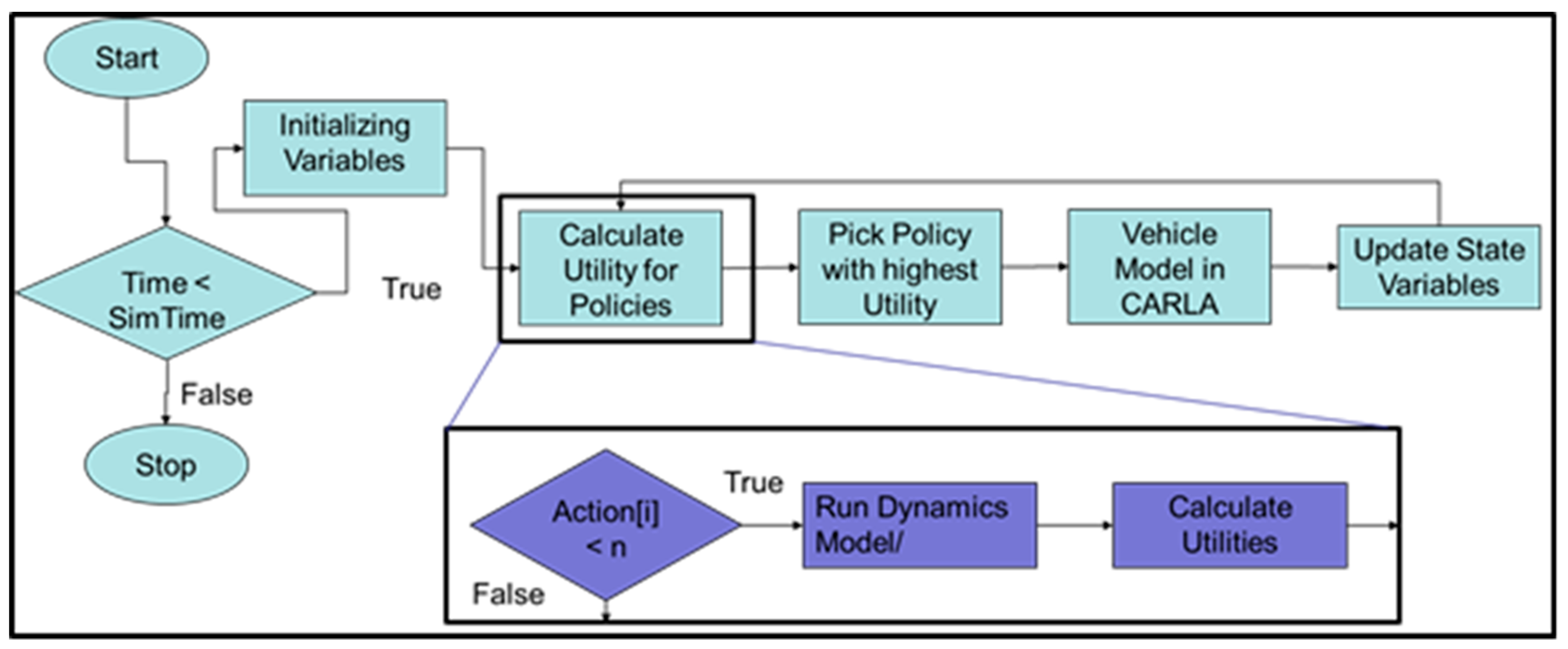
2.1. Developing a Utility Function for Resilient Decision Making

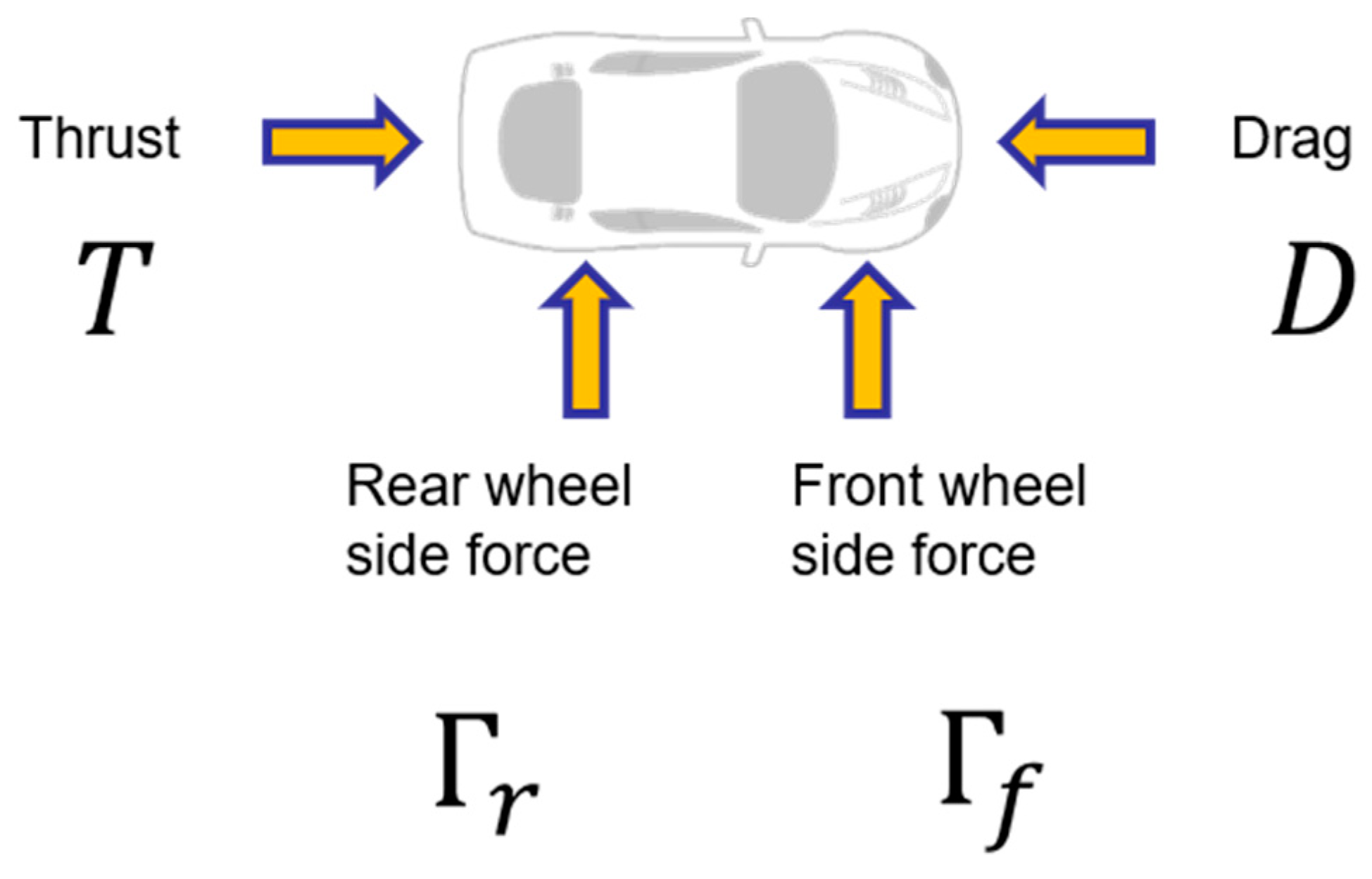
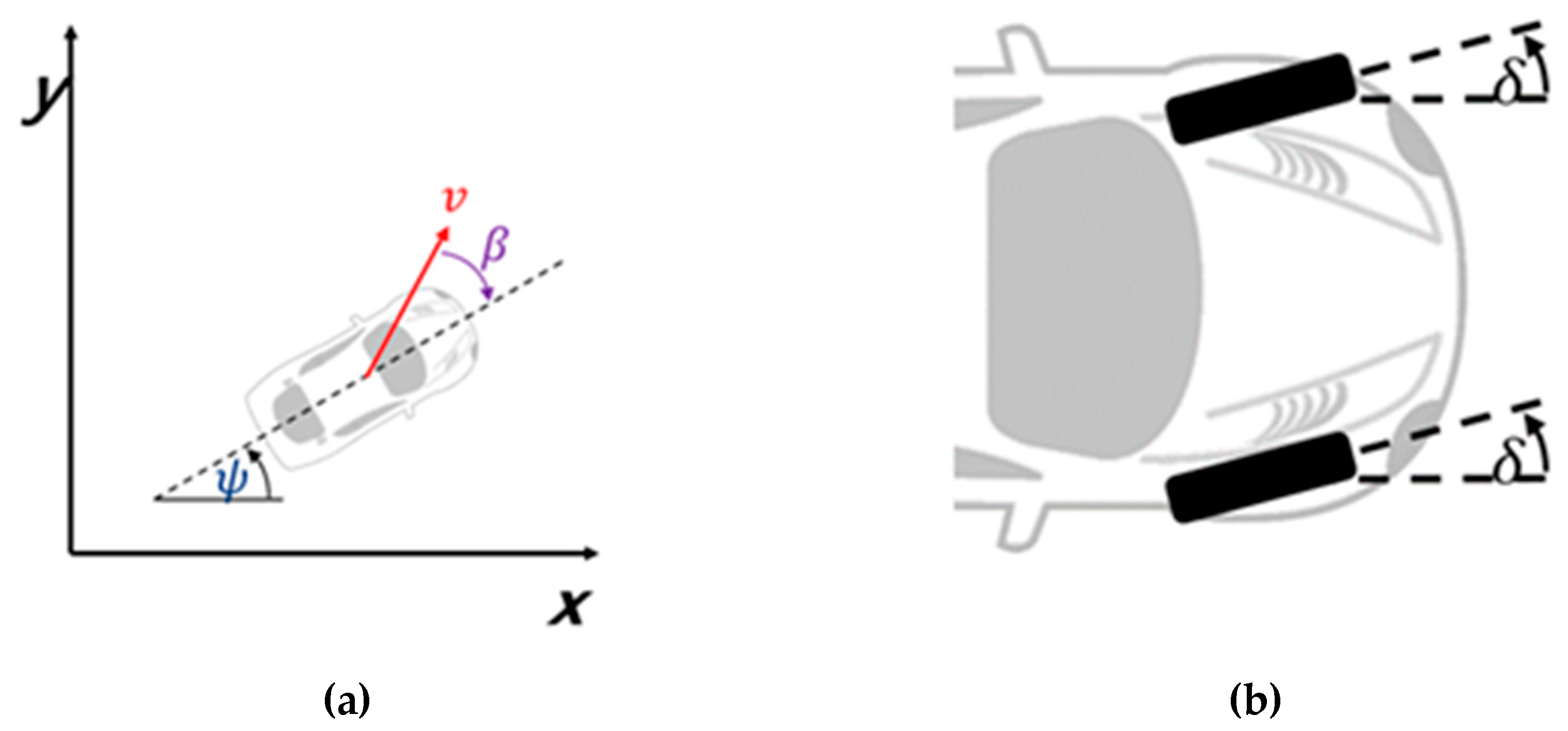
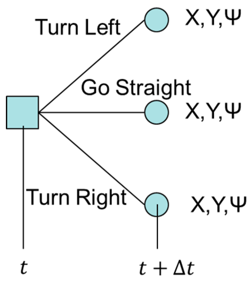
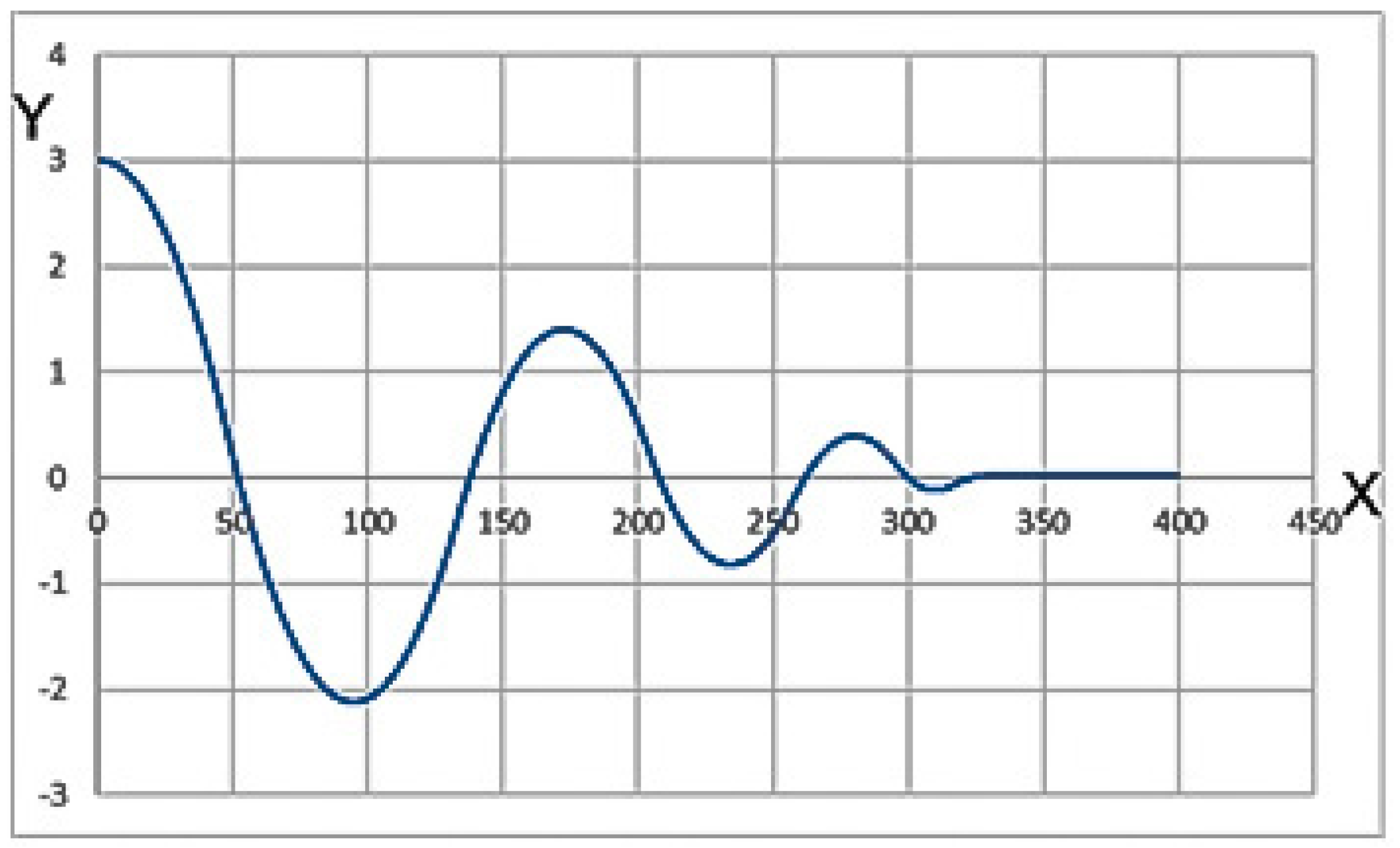
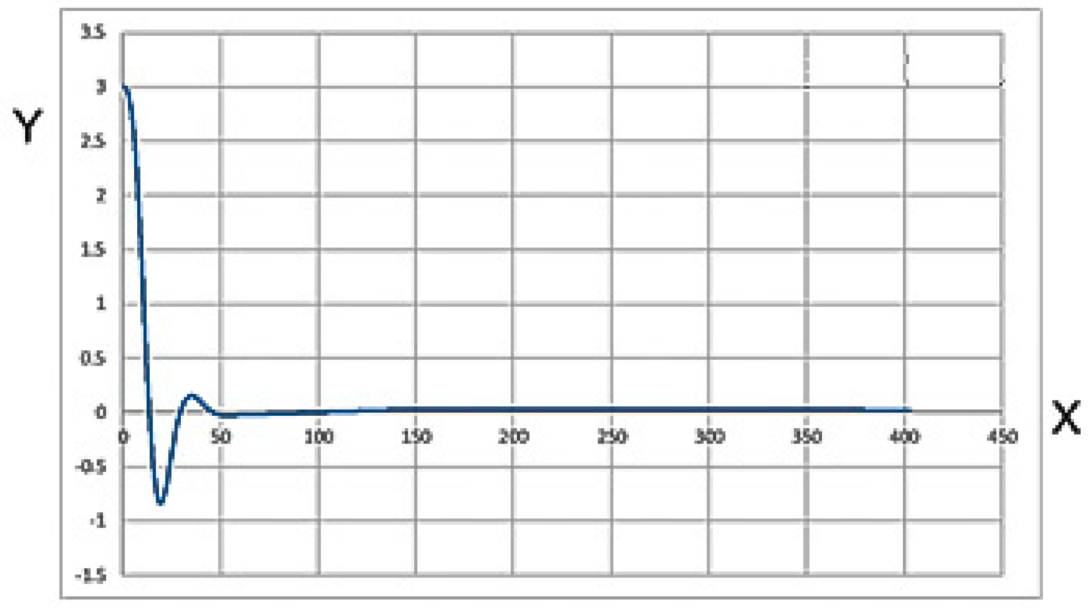
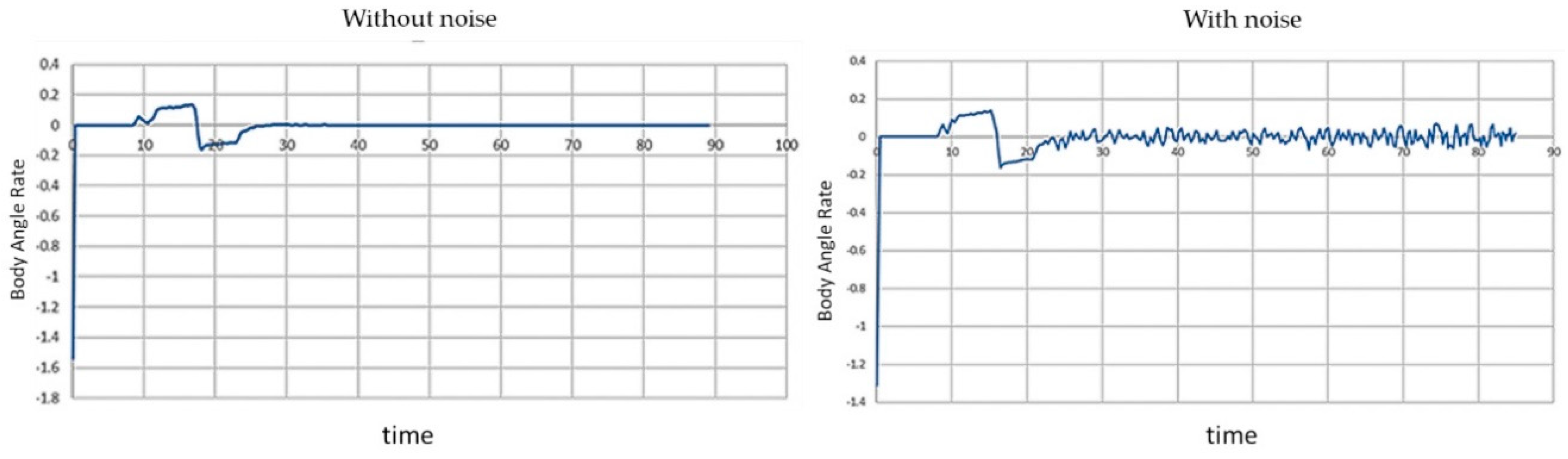
2.1.1. Dynamics Model

To develop a utility function a physics model with reasonable fidelity is required to support the decision-making process. This model helps determine the behavior of the system (i.e., expected outcome) and evaluate the alternatives (e.g., Turn Left, Turn Right, or go straight in lane centering application) based on that outcome. For example, for a lane centering application, which is discussed later, a bicycle model for vehicle dynamics is sufficient. For physics modeling, forces acting on the vehicle and the coordinate system are shown in Figure 1 and Figure 2, respectively.

The following 6 nonlinear equations (Equation (1)) give the physical state variables, assuming angles β and δ are small.

$$\begin{gathered} \dot{\beta }={\psi }^{\prime }+\frac{1}{mv}\left(\left[D-T\right]\beta -{\Gamma }_f-{\Gamma }_r\right) \\ \dot{\psi }={\psi }^{\prime } \\ \dot{{\psi }^{\prime }}=\frac{1}{\theta }\left({\Gamma }_f{l}_f-{\Gamma }_r{l}_r\right) \\ \dot{v}=\frac{1}{m}\left(T-D\right) \\ \dot{x}=v\cos \left(\psi -\beta \right) \\ \dot{y}=v\sin \left(\psi -\beta \right) \end{gathered}$$

(1)

where:

• β—Slip angle—Angle between car’s velocity vector and body angle
• ψ—Body angle—Angle of car’s centerline in global coordinate frame
• ψ′—Angular velocity—Derivative of body angle
• v—Velocity—Velocity in direction of centerline
• x—X position—X-position in global coordinate frame
• y—Y position—Y-position in global coordinate frame

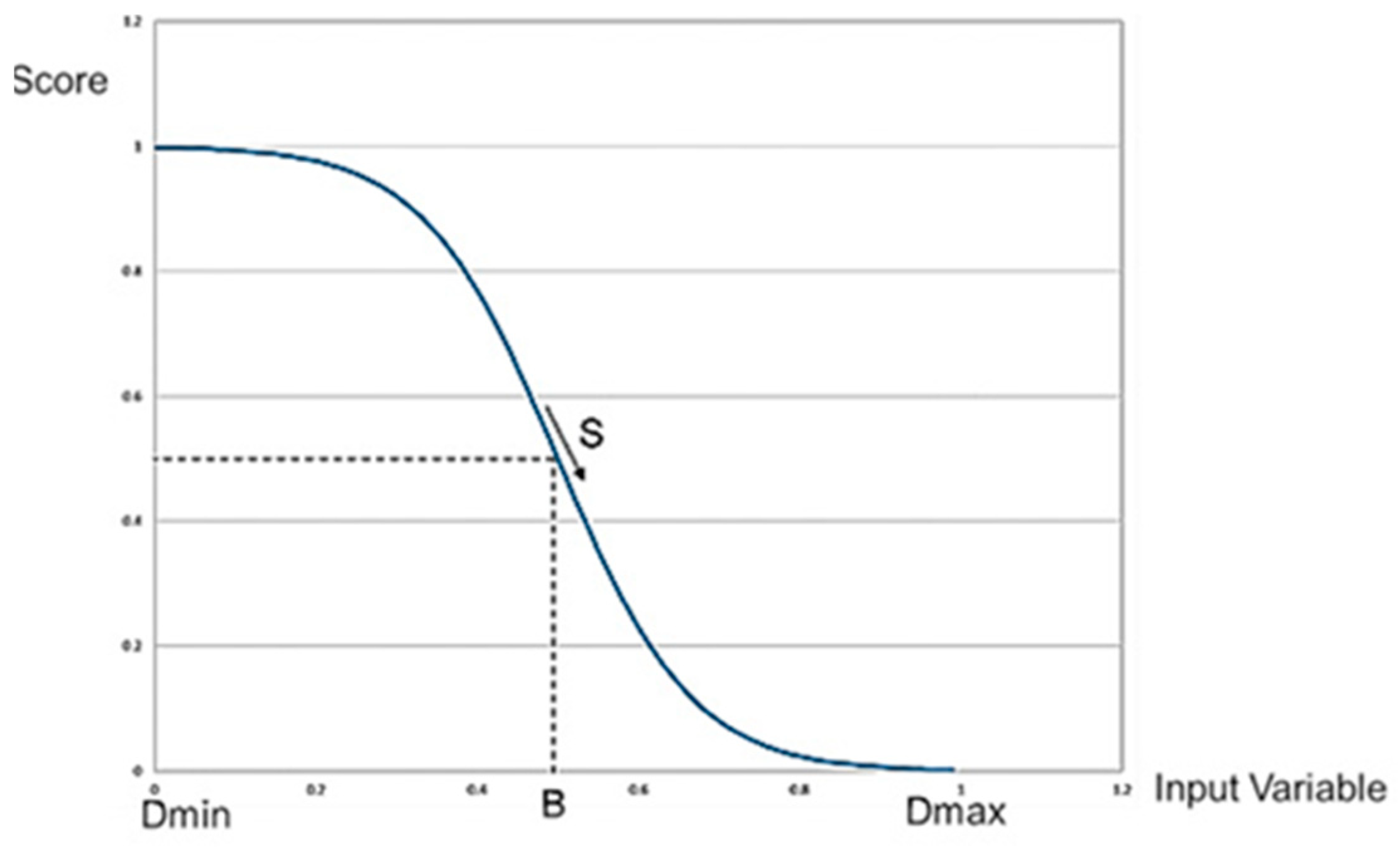
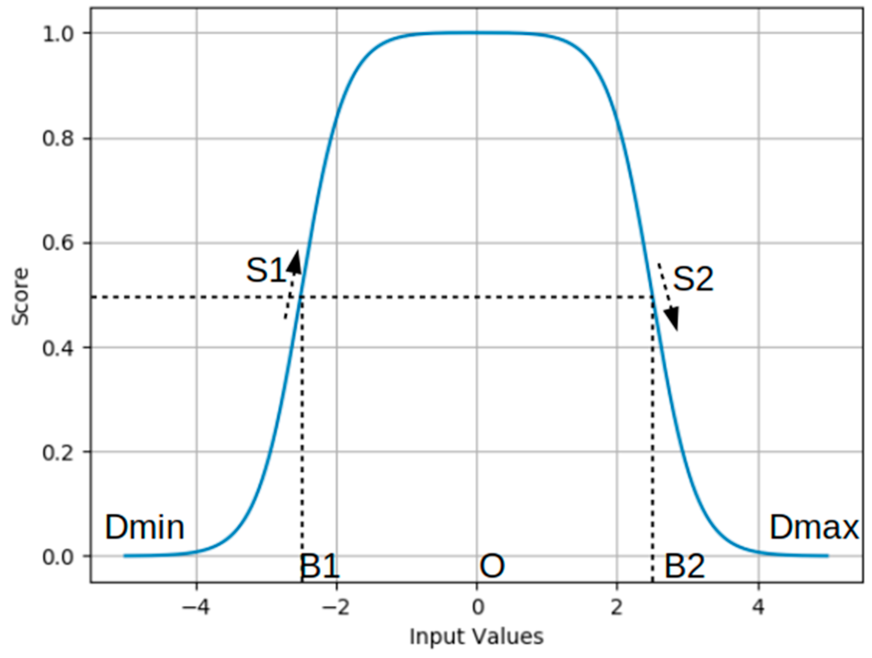
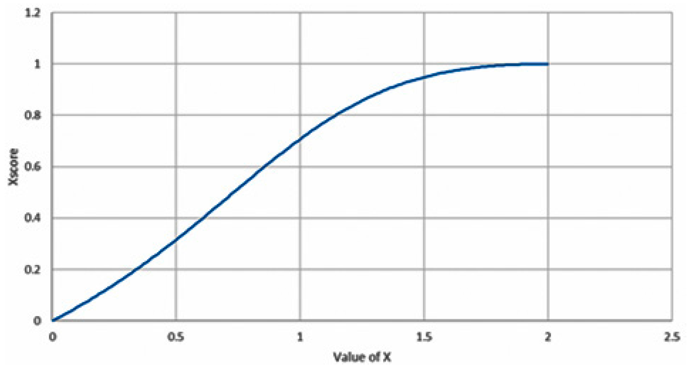
2.1.2. Constructing a Utility Function for Lane Centering

The goal of a vehicle lane centering application is to automatically steer the vehicle such that the vehicle maintains its position in the center of the current lane it is in as it travels down a road. For a simple version of such an application, the vehicle at each time t must make a decision from 3 alternatives: turn right, turn left, or go straight. These alternatives can then be instantiated in terms of policies. A policy is an action or set of action that the vehicle must take to achieve its goal (for example, turn right D degree, with T thrust). Figure 3 depicts vehicle’s decision making and alternatives in a simple decision tree.

To make a decision, the vehicle must evaluate potential outcomes before making the final decision and determine the utility (value) of the outcomes. The final decision will be the alternative with the highest utility and will be executed upon selection. This process happens in a loop until vehicle reaches its destination. Figure 4 shows the simulation flow.

To construct the utility function (Equation (2)), distance from the center line (Y), body angle (Ψ), and distance traveled in X direction were chosen as the attributes to be used in alternative evaluation.

$$\mathrm{Utility}=f\left(X,Y,\psi \right)$$

(2)

Furthermore, a linear sum of attributes utility function is utilized:

$$\mathrm{Utility}=w_{1}X+w_{2}Y+ w_3\psi ;w_1+w_2+w_3=1$$

(3)

However, these attributes need to be normalized since their units are different. Values of X and Y are in meters, and the value of ψ is in radian. Since X and Y are representing the position of the vehicle (specifically center of the mass), the vehicle’s position can be then represented by the vector R, where:

$$\left|\mathit{R}\right| = \sqrt{X^2+Y^2}$$

(4)

Values of X can be normalized by dividing X by R.

$$X_{norm}= \frac{X}{\mathit{R}} = X_{Score}$$

(5)

Figure 5 depicts the above equation (Equation (5)) assuming the value of Y goes to zero. As it can be seen, the overall function converges to 1.

The implication of this scoring function is “the more, the better”. As the value of X increases, the score of X increases. So, if the system was to simply pick an alternative for going straight, it would pick the alternative with the highest score of X.

To score the body angle Ψ a function where “less is better” is needed since it is desired to bring the vehicle body angle to zero (straighten the car eventually). To this end, a Wymore’s Standard Scoring Function (SSF) 10 [5] can be suitable to score these values. SSF 10 is shown in Figure 6.

SSF10 is given by the following function (Equation (6)):

$$\mathrm{Score}=1-\mathrm{SSF}4\left(B,-S,v\right)$$

(6)

$$S= - \frac{3}{\left|D_{max}-D_{min }\right|} ;B= \frac{D_{max}- D_{min}}{2}$$

where,

• B is called the baseline
• S is the slope of the function at the baseline
• v is the value of the input parameter, i.e., Ψ
• D_min and D_max are the maximum and minimum values of the input value
• SSF4(B,−S,v) is the Wymore’s 4th standard scoring function.

For brevity of analysis in this section the details of the SSF4 are not discussed here. Reader is referred to [5,6] for more details.

For lane centering, the Y value must converge to an optimal value of zero, essentially the center of the lane. Therefore, the optimal value of Y = 0 must receive the highest score (1) and as vehicle drives away from this value the score must be reduced, thus a bell shape curve can be constructed to score the values of Y. To this end, the standard scoring function 6 has the desirable characteristic. SSF6 is shown in Figure 7.

Furthermore, SSF6 is given using following equations (Equation (7)):

$$Score= \{\begin{array}{c}\frac{N}{1+N} y\ge O\\ \frac{P}{1+P} y<O\end{array}$$

(7)

where

$$N= {\left(\frac{B-O}{y-O}\right)}^{-2S_2\left(B+y-2O\right)}$$

$$P= {\left(\frac{O-B}{O-y}\right)}^{-2S_1\left(2O-y-B\right)}$$

In Equation (7), S₁ and S₂ are the slope of the function at the baselines B₁ and B₂, respectively. O is the optimal value that vehicle should converge to, y is the input value, and D_min and D_max are the maximum and minimum values of the input value, respectively.

Combining Equations (5)–(7), the full form of utility function is given in Equation (8).

$$Utility= \{\begin{array}{c}\frac{X}{\sqrt{X^2+Y^2}}+ \frac{N}{1+N}+\frac{R}{1+R} ; y\ge O,\psi \ge B_{\psi }\\ \frac{X}{\sqrt{X^2+Y^2}}+ \frac{N}{1+N}+\frac{1}{1+Q} ; y\ge O,\psi <B_{\psi }\\ \frac{X}{\sqrt{X^2+Y^2}}+ \frac{P}{1+P}+\frac{R}{1+R} ; y<O,\psi \ge B_{\psi }\\ \frac{X}{\sqrt{X^2+Y^2}}+ \frac{P}{1+P}+\frac{1}{1+Q} ; y<O,\psi <B_{\psi }\end{array}$$

(8)

where

$$Q= {\left(\frac{\frac{1}{\left|S\right|}}{B_{\psi }+\frac{1}{\left|S\right|}-\psi }\right)}^{2S\left(\frac{2}{\left|S\right|}-\psi +B_{\psi }\right)}, R== {\left(\frac{\frac{1}{\left|S\right|}}{-B_{\psi }+\frac{1}{\left|S\right|}+\psi }\right)}^{2S\left(\frac{2}{\left|S\right|}+\psi -B_{\psi }\right)}$$

$$N= {\left(\frac{B_2-O}{y-O}\right)}^{-2S_2\left(-2O+y+B_{2 }\right)}, P= {\left(\frac{-B_1+O}{-y+O}\right)}^{-2S_1\left(2O-y-B_1\right)}$$

The simulation results are discussed next. In these simulations, the utility function is calculated every 0.01 s. The rationale for calculating the utility function at such a high frequency is because this function is being used within the low-level control system and needs to be computed at a high rate to keep oscillations at the minimum. If the utility function is calculated at a lower frequency, due to the vehicle’s speed, oscillatory behaviors can appear.

Table 1. Policies Available to the Vehicle.

1. 0-Go Straight 0° 2. 1-Turn Left 0.66° 3. 2-Turn Right 0.66° 4. 3-Turn Left 1° 5. 4-Turn Right 1° 6. 5-Turn Left 2° 7. 6-Turn Right 2° 8. 7-Turn Left 5° 9. 8-Turn Right 5° 10. 9-Turn Left 10°

11. 10-Turn Right 10° 12. 11-Turn Left 15° 13. 12-Turn Right 15° 14. 13-Turn Left 20° 15. 14-Turn Right 20° 16. 15-Turn Left 25° 17. 16-Turn Right 25° 18. 17-Turn Left 30° 19. 18-Turn Right 30°

shows the list of all policies available to the vehicle.

Figure 8 show a simulation where only the first 3 policies are only available to the vehicle. To keep the problem simple the vehicle is keeping its velocity constant at 10 m/s, so the thrust value is adjusted accordingly. In this case, the vehicle makes many oscillations before converging to the centerline (Y = zero).

Figure 9 shows a simulation result where vehicle has all 19 policies available. As indicated in the figure, the vehicle shows better behavior. Thus, number of policies has an impact on the overall system behavior.

Next vehicle scenario simulations are performed within the CARLA simulation environment. The CARLA simulation environment is a simulation environment based on unreal engine 4 game-engine. The details of this simulation environment are discussed in [7].

Since the coordinate system in CARLA is reversed, then as the car drives straight the values of X decreases. The centerline where the vehicle needs to converge is at Y = 396. The diagram on the left side of Figure 10 shows the case where there is no noise in the feedback loop and the diagram on the right shows the simulation result where there is random noise in the feedback loop. The randomness is added using a unified random number generator and is added to the values of X and Y in the client side of the CARLA environment before sending these numbers to the utility function.

Figure 11 shows the comparison between the best action (best policy) between two cases. Policy number is plotted versus time. These policies are presented in Table 1.

Figure 12 compares the error versus time for both cases. The average steady state error with noise is very close to the steady state error in the without noise case. Eliminating the steady state error using this technique is part of future work.

Figure 13 shows the body angle rate change versus time. In both cases, it is very small. The average body angle rate in with noise case is 0.004 radians per second.

Based upon the results of our utility function decision making, we see that the scoring logic is important. The preference over alternatives must be known in order to construct the right form of the utility function. In the functions used here, the value of S in the scoring formula is basically the rate the system would change its preferences over alternatives given small inputs. There is a link between vehicle speed and slope of the utility function: faster speed requires lower S. The choices the system makes also changes with speed. For instance, when the initial speed is 10 m/s and initial position is 3 m to the left, turning 15° to the right is the best action. However, when initial speed is 20 m/s and initial position is 3 m to left, turning 10° to the right is the best action.

3. Simulation-Based Verification and Validation of Automotive Features

Verification and Validation of automotive features typically involves extensive on-the-road and/or simulation-based testing. Currently, major automakers and Silicon Valley-based companies spend a large amount of resources and time, driving millions of miles on public roads to gain confidence and establish trust in the autonomous capabilities of their vehicles. The challenge with on-road-testing is that it is hard to create and control a complete set of scenarios that involve factors such as traffic, adverse weather, and road conditions. In addition, it is difficult to determine an upper bound on the number of miles to drive to cover all possible events. Insufficient coverage of scenarios or unseen situations may put the autonomous system in hazardous situations.

To address these concerns, a simulation-based V&V approach for automotive features is commonly employed. The first step in the simulation-based V&V process involves generating a representative set of known scenarios mimicking different possible traffic conditions for testing. The safety and performance related properties against which the feature implementations need to be validated needs to be defined. Once the scenario is executed in simulation software or on a bench (with software/hardware-in-the-loop), the results need to be analyzed to validate whether the specified properties are satisfied.

The simulation-based V&V methodology requires the generation of a diverse set of scenarios validating automotive feature/system in terms of safety, performance, and reliability. For example, consider an adaptive cruise control (ACC) feature and the associated variables and values: weather—{clear, fog, snow, rain}, distance-to-vehicle-ahead—{near, mid, far}, traffic-density—{low, moderate, high}, time-of-day—{0, 1, …, 23} and target-cruise-speed—{45, …, 75} mph. Here the time-of-day and target-cruise-speed are continuous variables while others are discrete. Assuming we discretize the two continuous variables, for example time-of-day with 1-h increments and target-cruise-speed with 5 mph increments, the number of possible scenarios to simulate is 6048 (=4 × 3 × 3 × 24 × 7). Exhaustively simulating and verifying the full 6048 scenarios is a time-consuming task.

While a non-exhaustive approach is desirable to save time and resources, the challenge is to ensure coverage of all possible critical scenario cases to assess the vehicle behavior under extreme conditions and validate the feature implementation. We consider critical scenario cases that may be triggered by a clever choice of input parameter values and/or dynamic events encountered in the operation of the system.

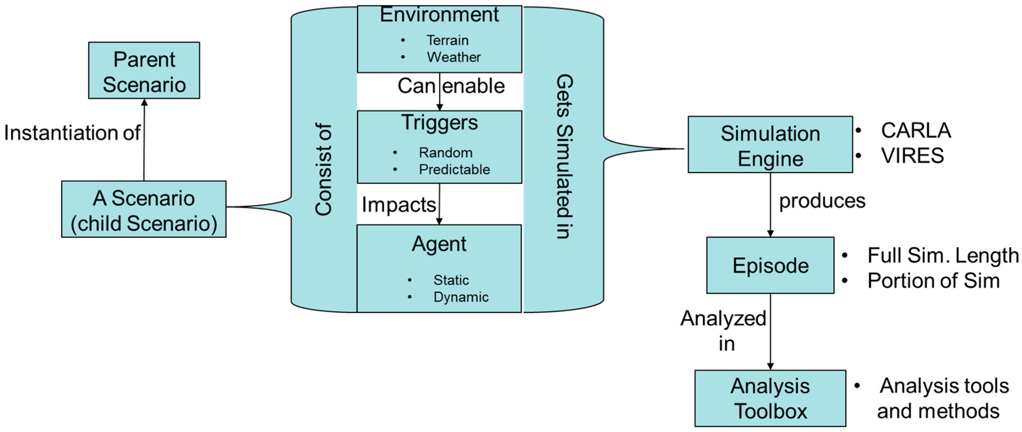
3.1. Simulation Environment Ontology for Automotive Systems

Figure 14 proposes an ontology for evaluation of a simulation environment in supporting the needs of our testing methodology.

A scenario is a segment, extended in time and space, involving the interaction of static and dynamic agents. It has a start and an end time as well as environmental conditions such as road and weather conditions. A parent scenario is a higher-level abstract description of a family of child scenarios; e.g., it may contain ranges of values rather than a specific value for a specific parameter. A child scenario can be created from a parent scenario, with a specific instantiation of the parameters of a parent scenario. It inherits all characteristics of the parent scenario but includes more details.

A scenario typically consists of an environment, triggers, and agents. An environment is essentially everything that is outside the vehicle under test (Ego vehicle). It includes environmental conditions such as terrain and weather as well as visibility which can be a function of both terrain and weather. The triggers are events that would cause disruption to the normal operation of the Ego vehicle. They can be associated with an agent in the environment or can come from the environment itself. Triggers can be random or deterministic in a specific scenario. They can be time-based or a consequence of an event in the simulation.

Agents are entities that exist within an episode. Agents can be static or dynamic. Static agents are stationary with no change in their position or behavior throughout the episode. Some examples of static agents are buildings, trees, road, sidewalks, road sign, construction zones, or a bridge. On the other hand, a dynamic agent is one that changes it state during the simulation. The examples of dynamic agents are the Ego Vehicle, other vehicles, two-wheelers, animals, birds, pedestrians, and automatic and manual traffic signals. Many behavior types can be associated with dynamic agents. For example, the vehicles can have behaviors associated with a conservative or an aggressive driver. An agent’s behavior is defined as a dynamic characteristic that results from the interaction of the agent with other agents, the environment, and/or internal states within the agent. The typical behavior of an agent can be periodic (e.g., traffic signal) or aperiodic (e.g., pedestrian jumping in front of the Ego vehicle) behavior.

The simulation engine is responsible for running the scenario and constructing the simulation episode. The simulation engine can be a platform enabling faster than the real-time simulation of an episode. This is essential for running multiple scenarios as fast as possible. An episode includes dynamic information including other vehicles, their trajectories, and dynamics, including the Ego vehicle dynamic information. It is the output of the simulation of the scenario. Each episode is basically a scenario with the details of the Ego vehicle and other agents or entities within the scenario. An episode can also be the entire simulation or a portion of the simulation. The episodes will then be analyzed in the analysis toolbox. This toolbox can include any kind of analysis algorithm that the engineer would wish to perform.

However, before setting up a scenario some questions need to be answered. For example, what is the purpose of that scenario? What is it trying to test? What are the parameters that can be varied in that scenario? How many child scenarios can be generated? What is/are the episode(s) we are interested in? Are we interested in the whole simulation or some portion of it? To perform analysis what are set of variables that can (or need to) be measured? In which units they should be measured—e.g., distance in meters, angles in radians, speed in meter-per-second?

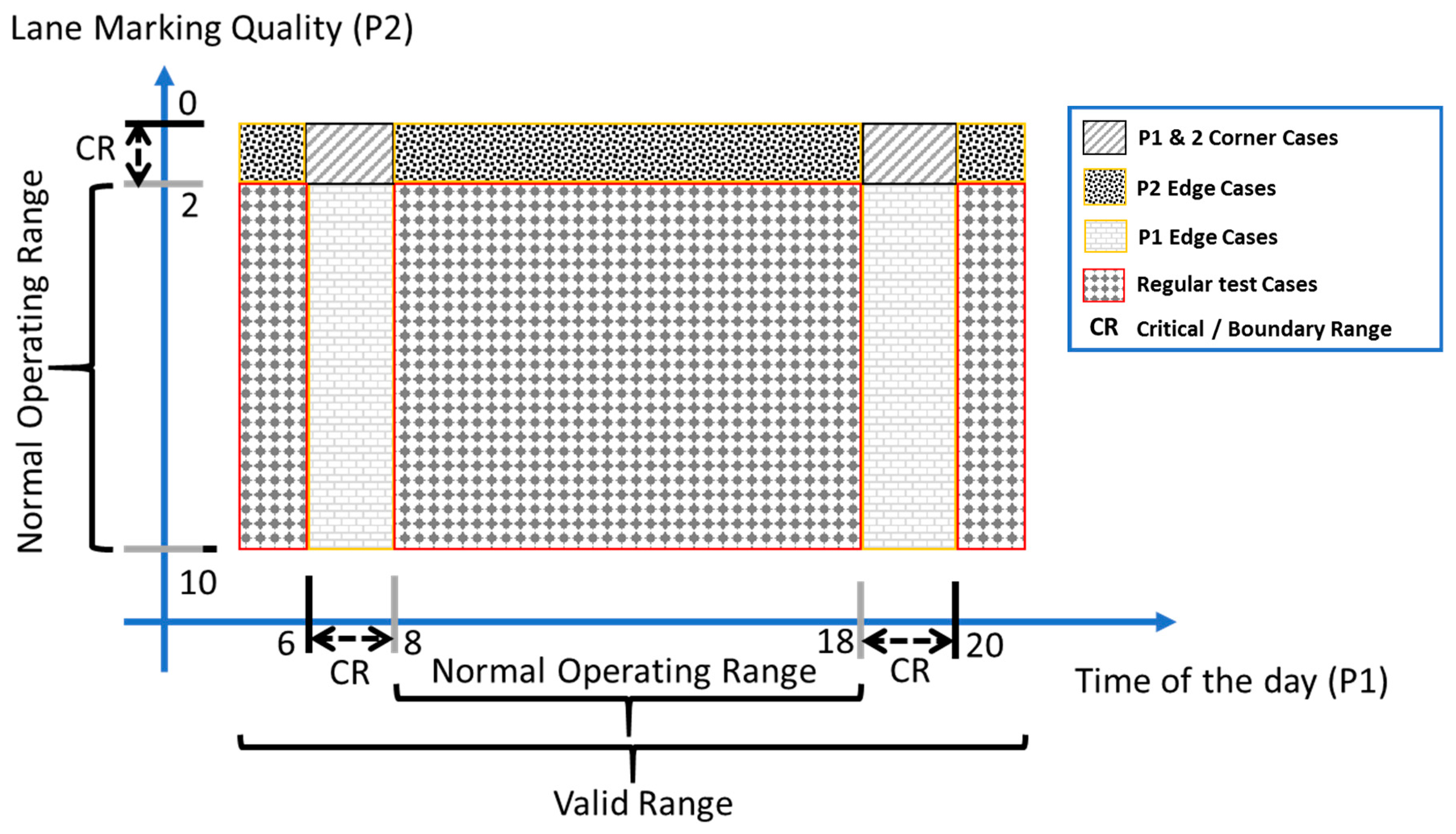
3.2. Definition of Testing Scenarios Classes

An automotive feature implementation typically involves a complex interaction of several vehicles and environment-related variables. In a simulation environment, each of the variables takes values from a pre-determined range (in the case of continuous variables) or a set (in the case of discrete variables). The specified range of variables is comprised of critical and non-critical operating regions based on the degree of influence of each variable/value on the correct system behavior. In addition, the system behavior is also dependent on other dynamic factors such as (mis-) behavior of other participating agents, environmental conditions, and dynamics.

3.2.1. Definition of Known Scenarios

In general, it is desirable to optimize testing by minimizing the number of scenarios while maximizing the coverage of the critical situations. The critical situations in each environment are defined by what is known as edge and corner cases. An edge case is defined to be a situation that occurs when one of the parameter values is at the boundary or critical operating region. Refer to

Table 2. Example Scenarios Parameters.

Parameter	Value Range	Non-Critical Range	Critical Range
Time of the Day	0 to 24	All except 6 to 8 & 18 to 20	6–8 h & 18–20 h (high reflection & Glare due to sun rise & set)
Vehicle Speed	0 to 90 mi/h	30 to 60	0 to 29 & 61 to 90
Lane Marking Quality	0 (Bad) to 10 (good)	3 to 10	0 to 2

for a critical and non-critical value range example. In this table the parameter “Time of the day” is given as 0 to 24:00, and the critical range is defined as 6–8 Hrs and 18–20 Hrs as reflection and glare may occur due to sun rise and sun set. Nevertheless, the critical region does not need to be in both sides of the value range as indicated for the parameter “Lane Marking Quality” in Table 2.

A corner case is defined to be a situation that occurs when more than one parameter is simultaneously in the boundary or critical operating region. Figure 15 pictorially illustrates the definitions provided above. Parameter 1 (P1) “Time of the day” is plotted in the X-axis and the parameter 2 (P2) “Lane Marking Quality” is plotted in the Y-axis and the critical ranges are marked respectively. The regions “6 to 8” and “18 to 20” in parameter 1 are the edge cases of it, as long as the parameter 2 value is within the normal operating range. If both the parameters values are in their critical region then it is marked as the corner cases. Trivially, the coverage of the critical ranges should be increased by generating more edge and corner case scenarios to effectively validate the system. Of course, the critical region of any parameters may differ based on the behavior or the system. For example, to validate the behavior of the system in the summer night hours then the critical region of the parameter “Time of the day” may change to 20–5 Hrs.

3.2.2. Definition of Unknown Scenarios

Automotive system behavior does not only depend on the environmental elements but also on the dynamic behaviors of other participating agents in that environment. Some examples of such events are:

• A participating vehicle moving towards the Ego Vehicle lane or cutting across the lane
• A child runs in front of the Ego Vehicle from a hidden area
• Rock or landslide in front of the Ego Vehicle
• Mal/not functioning traffic lights
• A traffic rule breaking participating vehicle
• Procession/convoy that stops the Ego Vehicle to follow the traffic rules

We classify such potential but rarely occurring events as unknown scenarios and posit that it is important to simulate and validate the vehicle behavior for such events as well. The number of participating agents in any of the events can be many and varying. Therefore, it would be precise to model the situation as an event(s) incident on the Ego Vehicle as caused by one or more agents instead of participating agents’ parameters. The simulation of such unknown scenarios under various categories is a work in progress. We plan to generate such scenarios by introducing randomness in the input parameters and their combinations.

3.3. Test Scenario Generation for Simulation

In this section, we describe different techniques for test scenario generation. The random testing technique involves random sampling of input parameter value ranges according to a chosen probability distribution [8,9]. Test scenario generation using this technique is simple and may be useful in the detection of faults that are overlooked by more systematic techniques. Nevertheless, this technique may require a large set of scenarios to be tested for effectively identifying extreme cases.

A structural technique [10] exploits the internal structure of the system to define a coverage criterion. In addition, an adequacy criterion is defined for scenarios used for structural testing specifying that they must exercise each coverage element at least once. Statistical testing [11] combines random and structural techniques. Here, the test scenarios are obtained via random sampling, but the probability distribution must satisfy the specified adequacy criterion.

Orthogonal array testing (OAT) is a well-known method in software testing to ensure system reliability. The basic idea is that most system faults result from the interaction of more than one parameter [12]. Unlike a typical software program, the dynamics of an autonomous feature implementation is impacted by the external factors incident on the system. To study such interaction behavior, OAT is a more suitable technique compared to purely random-based or statistical techniques that deal with a single parameter at a time. A t-way interaction testing based on the IPOG algorithm ensures all t-parameter values are covered by at least one test in the test set. Studies show that most faults are triggered by 2 ≤ t ≤ 6-way interactions. An IPOG-based 2-way (aka pairwise) testing for the ACC example results in 169 test scenarios, a significant reduction from the exhaustive 6048 possible scenarios.

To ensure the coverage of edge/corner cases, besides OAT, we employ optimization algorithms such as simulated annealing and random restart hill climbing. The algorithm fuzzes the parameter values obtained by employing OAT to generate new combinations in such a way that potentially result in the identification of edge/corner cases if any.

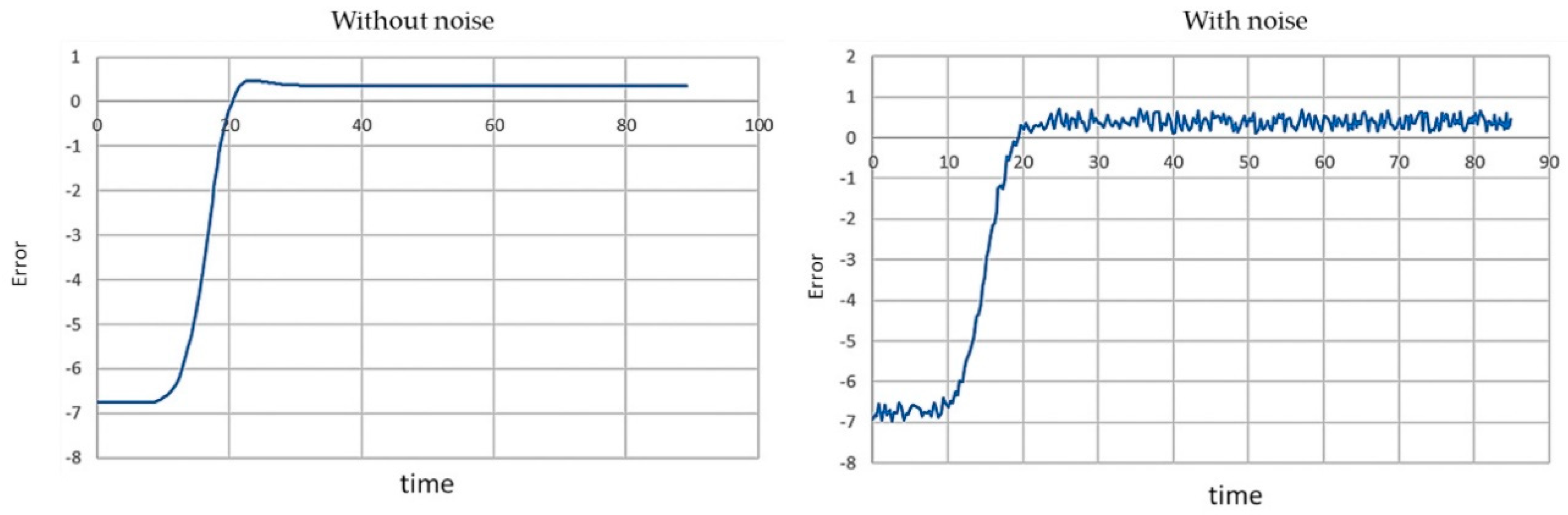
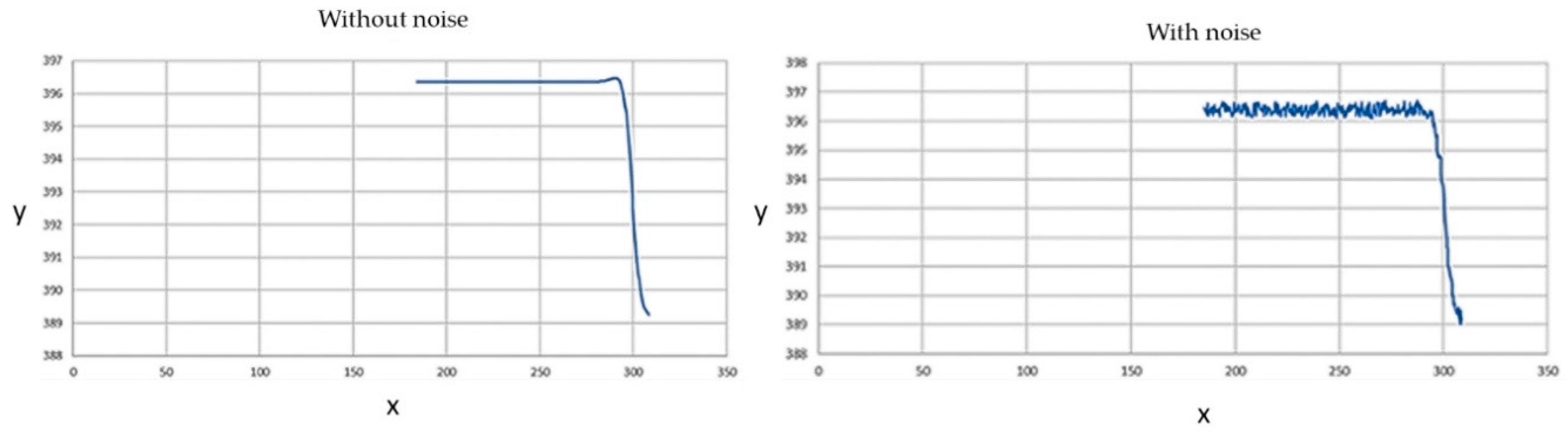
3.4. Monitors for Simulation Episode Analysis

Once a library of test scenarios has been generated by employing the OAT technique, suitable scenario implementation files for the chosen simulation engine (e.g., VIRES-VTD, CARLA, …) needs to be produced. The simulation is then executed, and the results are collected using simulation engine APIs. The results typically indicate the positions of the host vehicle and other objects (including other vehicles on the road, pedestrians, traffic signals, and signs, etc.), their speed of movement, its distance to the host vehicle, and so on. The collected results may be stored in the desired format for offline analysis. The analysis would uncover violations of the safety or performance properties (if any) implemented as monitors. Alternatively, the monitors may be implemented to flag property violations online, i.e., during the simulation run as and when the events occur.

An example of a safety monitor for the ACC feature is the validation of the gap between the host vehicle and other objects. This safety property may raise a flag if other objects in the simulated environment come within the radius of the user-supplied gap setting (near/mid/far). Under such circumstances, the host vehicle should adjust its speed to avoid the collision.

The validation results are then supplied to the vehicle control algorithm developers who may then diagnose the source of faults or tune the algorithm parameters for improved safety and performance.

4. Discussion and Conclusions

In this paper, we have shown our recent developments in our MBSE approach for modeling and simulation of automated automotive systems. Within the Resilience Contract framework, we specifically discussed the development of utility functions and showed how these functions can be developed for lane centering systems. Furthermore, we have shown simulation results within the CARLA simulation environment.

We next discussed the recent developments in simulation-based verification and validation approaches. We argued that rigorous modeling and extensive simulation-based testing are essential for the validation of next-generation automotive systems and software. We also discussed the benefits of modeling and simulation of some simple versions of automotive systems. The problem of validation targeted toward identifying unknown situations and cases where a system can fail is indeed challenging. A careful combination of systematic and random testing needs to be employed to detect the possible malfunctions arising out of errors in the system requirements, design, and implementation, and technology limitations of sensors and the inherent incomplete comprehension of environments.

These two main discussion points in this paper are complimentary. Resilience Contracts need to be tested within the simulation environment and the V&V approach can lead to the development of scenarios where these resilience contracts can be tested and trained. The training is specifically associated with the POMDP within the RC construct. For example, various scenarios can help to fine-tune transition probabilities and reward functions that exist within the Resilience Contract construct.

The future work that needs to be done is to develop an integrated framework between Resilience Contracts and V&V methodology discussed in this paper.

References

1. ISO 26262 Road Vehicles—Functional Safety; International Organization for Standardization: Geneva, Switzerland, 2011.
2. ISO PAS 21448 Safety of the Intended Functionality; International Organization for Standardization: Geneva, Switzerland, 2018.
3. Madni, A.M.; Sievers, M.W.; Humann, J.; Ordoukhanian, E.; D’Ambrosio, J.; Sundaram, P. Model-Based Approach for Engineering Resilient System-of-Systems: Application to Autonomous Vehicle Networks. In Disciplinary Convergence in Systems Engineering Research; Madni, A., Boehm, B., Ghanem, R., Erwin, D., Wheaton, M., Eds.; Springer: Cham, Switzerland, 2018. [Google Scholar]
4. Madni, A.M.; Sievers, M.W.; Humann, J.; Ordoukhanian, E.; Boehm, B.; Lucero, S. Formal Methods in Resilient Systems Design: Application to Multi-UAV System-of-Systems Control. In Disciplinary Convergence in Systems Engineering Research; Madni, A., Boehm, B., Ghanem, R., Erwin, D., Wheaton, M., Eds.; Springer: Cham, Switzerland, 2018. [Google Scholar]
5. Wymore, A.W. Model-Based Systems Engineering; CRC Press: Boca Raton, FL, USA, 1993. [Google Scholar]
6. Daniels, J.; Werner, P.W.; Bahill, A.T. Quantitative methods for tradeoff analyses. Syst. Eng. 2001, 4, 190–212. [Google Scholar] [CrossRef] [Green Version]
7. Dosovitskiy, A.; Ros, G.; Codevilla, F.; Lopez, A.; Koltun, V. CARLA: An Open Urban Driving Simulator. In Proceedings of the 1st Annual Conference on Robot Learning, Mountain View, CA, USA, 13–15 November 2017; pp. 1–16. [Google Scholar]
8. Duran, J.W.; Ntafos, S.C. An evaluation of random testing. IEEE Trans. Softw. Eng. 1984, 4, 438–444. [Google Scholar] [CrossRef]
9. Zhu, H.; Hall, P.A.; May, J.H. Software unit test coverage and adequacy. ACM Comput. Surv. 1997, 29, 366–427. [Google Scholar] [CrossRef]
10. Denise, A.; Gaudel, M.C.; Gouraud, S.D. A generic method for statistical testing. In Proceedings of the IEEE International Symposium on Software Reliability Engineering, Bretagne, France, 2–5 November 2004; pp. 25–34. [Google Scholar]
11. Cohen, M.B.; Gibbons, P.B.; Mugridge, W.B.; Colbourn, C.J. Constructing test suites for interaction testing. In Proceedings of the International Conference on Software Engineering, Portland, OR, USA, 3–10 May 2003; IEEE Computer Society: Washington, DC, USA, 2003; pp. 38–48. [Google Scholar]
12. Kuhn, D.R.; Wallace, D.R.; Gallo, A.M. Software fault interactions and implications for software testing. IEEE Trans. Softw. Eng. 2004, 30, 418–421. [Google Scholar] [CrossRef]
Figure 1. Forces acting on the vehicle.
Systems 07 00001 g001
Figure 2. (a) Coordinate system and (b) Vehicle steering angle.
Systems 07 00001 g002
Figure 3. Decision Tree.
Systems 07 00001 g003
Figure 4. Simulation Flow.
Systems 07 00001 g004
Figure 5. Score of X vs. Value of X as Y approaches to zero.
Systems 07 00001 g005
Figure 6. Standard Scoring Function 10.
Systems 07 00001 g006
Figure 7. Standard Scoring Function 6 for scoring Y values.
Systems 07 00001 g007
Figure 8. Simulation results when 3 policies are only available.
Systems 07 00001 g008
Figure 9. Simulation results when 19 policies are only available.
Systems 07 00001 g009
Figure 10. Simulation Results, Position Graphs.
Systems 07 00001 g010
Figure 11. Simulation Results, Best Action vs. Time.
Systems 07 00001 g011
Figure 12. Simulation Results, Position Error vs. Time.
Systems 07 00001 g012
Figure 13. Simulation Results, Body Angle Rate vs. Time.
Systems 07 00001 g013
Figure 14. Simulation Ontology.
Systems 07 00001 g014
Figure 15. Illustration of regular, edge, and corner cases.
Systems 07 00001 g015