Vit-Traj: A Spatial–Temporal Coupling Vehicle Trajectory Prediction Model Based on Vision Transformer

Abstract

Accurately predicting the future trajectory of road users around autonomous vehicles is crucial for path planning and collision avoidance. In recent years, data-driven vehicle trajectory prediction models have become a significant research focus, and various spatial–temporal neural network models, based on spatial–temporal data, have been proposed. However, some existing spatial–temporal models segregate time and space, neglecting the inherent coupling of time and space. To address this issue, an end-to-end spatial–temporal feature fusion model, based on the Vision Transformer (Vit), is proposed in this paper, which can couple stereoscopic features of diverse spatial regions and time periods. Specifically, we propose an end-to-end spatiotemporal feature coupling model based on visual Transformer, Vit-Traj, which extracts spatiotemporal features through 2D convolution and uses Vit and SENet to complete feature fusion. Experimental results on the NGSIM and HighD datasets indicate that, compared to State-of-the-Art models, the proposed model exhibits better performance. The root mean squared error (RMSE) is 2.72 m on the NGSIM dataset and 0.86 m on the HighD dataset when the prediction horizon is 5 s. Furthermore, ablation experiments are conducted to evaluate the performance of each module, affirming the efficacy of ViT in modeling spatial–temporal data.

1. Introduction

Autonomous driving can significantly improve the traffic efficiency and safety of roads. Autonomous vehicles (AVs) perceive the surrounding road environment through sensors and predict future situations based on the perceived information [1,2]. The trajectory prediction of traffic participation around target vehicles is a crucial step in achieving autonomous driving [3,4]. Trajectory prediction is an uncertainty issue, so multi-modal trajectory prediction is also highly valued by people [3,5].

In general, trajectory prediction is a time series forecasting problem, the goal of which is to extract features from past trajectories within a certain period and then use these features to predict future trajectories. Historical trajectory data are commonly in the form of time series data, so some sequence models, such as RNN, transformer, etc., are used for trajectory prediction [6]. However, in the real world, the traffic environment in which vehicles operate is very complex. There are often multiple types of traffic participants, such as pedestrians, electric vehicles, bicycles, etc. When predicting trajectories, it is necessary to consider the impact of surrounding traffic participants on the target vehicle being predicted. This introduces a spatial dimension on top of the time dimension, making it challenging for some sequence models to handle this type of structured data.

Therefore, spatial–temporal models and spatial–temporal data have become research hotpotS, leading to the development of deep learning models based on spatial–temporal data. In the spatial dimension, it is necessary to consider the relationships between different traffic entities in various regions and then aggregate information features from the traffic entities. But the inherent graph structure in space could limit information propagation along the edges [7]. In other words, when performing feature fusion between nodes, they can only propagate based on the edges, which makes it difficult for some nodes to have comprehensive interaction, and is like an attention mechanism with natural biases to nodes. In the time dimension, various sequence models can be utilized, such as the RNN model.

However, most of these spatial–temporal models separate time and space, with fewer models considering the coupled features of time and space. Hence, it is necessary to simultaneously couple spatial and temporal features and utilize them for downstream tasks. Spatial–temporal data have a similar structure to image data. We can treat the spatial dimension of spatial–temporal data as the channel dimension of image and use some 2D convolutional kernels to extract features from different spatial nodes simultaneously, combining them into a feature map.

Due to the strong performance of the transformer in large language models, the transformer has also been applied in vision tasks, leading to the development of the Vision Transformer (ViT) [8,9]. ViT divides images into patches, converts these patches into token sequences using a certain tokenize method, and then fuses them using a transformer. Therefore, ViT can be used to extract the correlations between different spatial features of image and output the fused features from different image patches. An earlier precursor to ViT is SENet [10], which globally pools the feature maps into scalars, calculates the importance of each feature map channel using fully connected layers and sigmoid, aggregates information from different patches, and achieves a good feature extraction ability while having fewer parameters.

Considering that some existing research has overlooked the spatial–temporal coupling features of traffic participant and some deficiencies in spatial feature information aggregation and transmission, this paper proposes a trajectory prediction model that couples spatial–temporal data of surrounding vehicles in the target area. This model can simultaneously fuse the feature in the time and space dimensions, addressing existing shortcomings. Therefore, the main contributions of this paper are as follows:

• Spatial–temporal coupling features of trajectory spatial–temporal data are extracted using 2D convolutional kernels, capturing the feature relationships of different nodes and periods.
• 2D feature maps of different spatial–temporal segments are fused using ViT and SENet, obtaining a fusion feature map between different periods and spaces.
• By integrating the aforementioned advantages, an end-to-end vehicle trajectory model, the Vit-Traj model, was proposed and experimentally demonstrated to exhibit good performance.

2. Related Work

Many studies have conducted research on vehicle trajectory prediction problems, which can be divided into the following categories.

2.1. Physical Mathematical Models

These physical and mathematical models treat vehicles as point masses and formalize their motion behaviors using physical relationships [11]. In addition, some car-following models are also used to predict the trajectory between the front vehicles and rear vehicles [12,13]. However, these physical and mathematical models are overly idealized and are difficult to apply to complex real-world traffic scenarios [3].

2.2. Machine Learning Models

Machine learning methods aim to learn patterns from data and often rely on the statistical distribution characteristics of the data, using techniques such as Gaussian processes [14,15], Kalman filtering [16,17], and Hidden Markov Model [18], among others.

These models typically predict future trajectories by correcting the current trajectory using posterior estimation. Their drawback is that they struggle to perform nonlinear modeling and adapt to increasingly complex traffic environments and high-dimensional data.

2.3. Deep Learning Models

Deep learning models are data-driven models that can handle various structured and high-dimensional data. In vehicle trajectory prediction, common models include sequence models such as the RNN series (LSTM [19,20], GRU [21,22], BiLSTM [23], and their variants), sequence models like the self-attention, transformer, and combination models of the CNN1D and RNN series, such as CNN-LSTM [24,25].

In terms of input and output, multi-variable inputs have become mainstream compared to single-feature variable inputs [26,27]. Additionally, multi-variable multi-output models are more favored by researchers [28]. For loss functions, commonly used ones include MAE, MSE, and RMSE, among others. There is also a loss in functions based on feature distribution similarity, as seen in [24,29,30].

Trajectory prediction based on deep learning models can be summarized as a time series prediction problem [31]. Although it can achieve good prediction performance, there are still some issues that need to be urgently addressed in the future. For example, they ignored the interaction between different entities and only modeled from the time dimension, ignoring the relationships between different variables.

2.4. Spatial–Temporal Neural Network Models

Models based on spatial–temporal data are often deep neural network models as well. These models achieve higher performance because they consider the interaction between traffic participant entities (spatial dimension) and temporal dimensions such as periodicity and autocorrelation. Due to the dimensions of spatial–temporal data containing spatial and temporal dimensions at the same time, they do not conform to the input of general sequence data. Therefore, some models that can handle spatial–temporal data have been proposed [32,33,34].

In the spatial dimension, it is necessary to consider the relationships between traffic entities in different regions and then aggregate information features from these traffic entities. Common methods include graph convolutional neural networks (GCN) [10,35,36,37] and self-attention mechanisms [32]. On one hand, self-attention mechanisms are used to adaptively aggregate information from the feature for each node. On the other hand, GCN relies on a priori given graph structure for information propagation, which limits the effectiveness of GCN, as it is strongly constrained by the graph structure. Although it can dynamically learn the relationships between nodes by using self-attention mechanisms and obtaining some edge attributes [38,39], it is also difficult to solve this problem [7]. In the temporal dimension, various sequence models can be used, such as RNN series models [40] and efficient transformer models [41].

Table 1. Summary of different method models in related work and introduction.

Model	Input	Output
Physical mathematical models	Speed, position, acceleration etc.	Short term trajectory
Machine learning models	one-dimensional cross sectional data	Short term trajectory
Deep learning models	Multivariate time series or Multi targets univariate time series	Mid-term trajectory and long-term trajectory
Spatial–temporal neural network model	Multi targets multivariate time series and Graph	Mid-term trajectory and long-term trajectory

summarizes the different methods and models used in the relevant work and introduction, listing their input and output as well as the length that can be predicted. However, most of these spatial–temporal models separate time and space; only a few models consider the coupling features of time and space simultaneously. Some models also obtain the final feature vector by fusing the features of time and space [42,43]. However, they only perform feature addition or concentration before feeding the features into the fully connected layer, which does not simultaneously account for the coupling of temporal and spatial features.

2.5. Trajectory Prediction Using HighD and NGSIM Datasets

In the realm of vehicle trajectory prediction, the NGSIM and highD datasets have been widely employed to evaluate and enhance the accuracy of predictive models. Cai et al. [44] utilized the NGSIM and highD datasets to propose an Environment-Attention Network (EA-Net), which integrates a parallel structure of Graph Attention Network (GAT) and Convolutional Social Pooling with Squeeze-and-Excitation mechanism (SE-CS) to capture the comprehensive interaction between the vehicle and its driving environment. Their model demonstrated superior performance, achieving a prediction accuracy improvement of over 20% compared to single-structure models. Similarly, Xu et al. [45] developed a Group Vehicle Trajectory Prediction model with a Global Spatio-Temporal Graph, leveraging the NGSIM US-101 and I-80 datasets to construct a complex network that captures the spatio-temporal features of vehicle trajectories. Their approach achieved a 16.6% higher accuracy in long-term predictions compared to other advanced schemes. In another study, Xing et al. [46] focused on personalized vehicle trajectory prediction for connected vehicles, using the NGSIM dataset to develop a joint time-series modeling approach based on long short-term memory (LSTM) networks. They recognized different driving styles using the Gaussian mixture model (GMM) and proposed a personalized trajectory prediction framework that outperformed baseline algorithms in terms of prediction accuracy. These studies collectively highlight the significance of utilizing comprehensive datasets like NGSIM and highD to advance the field of vehicle trajectory prediction through innovative modeling techniques and enhanced interaction analysis.

3. Preliminary

3.1. SENet

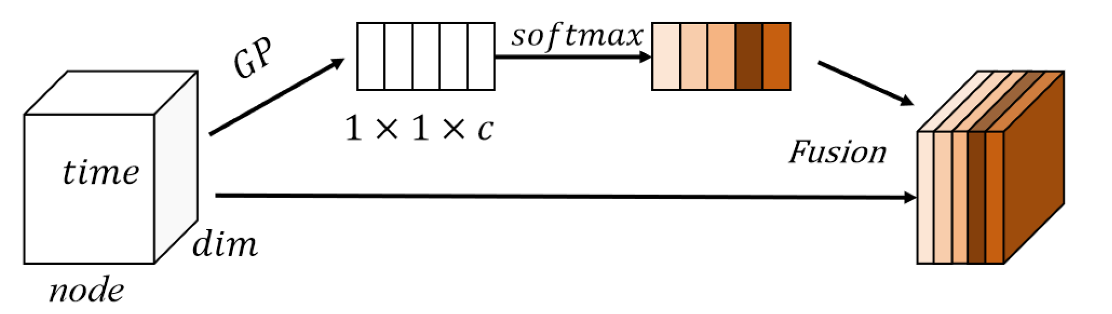
SENet (Squeeze-and-Excitation Network) is an attention mechanism used to enhance the performance of deep convolutional neural networks (CNNs). It adaptively adjusts the correlations between channels by learning the weights for each channel, thereby improving the expressive power of the model.

The core idea of SENet is to weight the feature maps of CNNs using an attention mechanism called the “Squeeze-and-Excitation” module. This module consists of two main operations, namely Squeeze and Excitation, as shown in Figure 1. SENet first squeezes the channel dimension by global pooling, then calculates the importance of each channel, and finally expands it to its original shape.

In the Squeeze operation, SENet compresses the feature maps of each channel into a single value by using global average pooling. This represents each channel as a global feature that reflects its importance to the overall feature, as shown in Formula (1), where $u_c$ is a channel, $zc$ is squeeze value of channel $u_c$, $H$ and $W$ are the height and width of the feature map, respectively.

$$zc=F_{sq}\left(u_c\right)={\displaystyle \frac{1}{H\times W}}{\displaystyle \sum _{i=1}^{H}su{m}_{j=1}^W}{u}_c\left(i,j\right)$$

(1)

In the Excitation operation, SENet learns the weights for each channel through two fully connected layers. The first layer maps the global feature to a smaller dimension and applies a nonlinear transformation using an activation function like ReLU. The second layer maps this smaller dimension back to the original number of channels and generates weights between 0 and 1 using a sigmoid function. This weight vector is then applied to each channel of the original feature maps to adjust their importance. The formula for the Excitation operation is shown in Formula (2), where $W$, $W_1$, and $W_2$ represent the learnable parameter. In the process of gradient descent, the model can automatically determine the optimal weight values between the channels.

$$s=F_{ex}\left(zc,W\right)=\sigma \left(W_2\delta \left(W_1\times zc\right)\right)$$

(2)

By introducing the SENet module, CNNs can learn the weights for each channel adaptively, enhancing important feature channels while suppressing less important ones. This attention mechanism improves the model’s expressive power and generalization ability, thereby enhancing its performance.

In this paper, SENet is used to fuse features between different feature channels (feature maps). Specifically, each feature map represents different aspects of features, which clearly have certain relationships, and SENet can perfectly extract this relationship.

3.2. Vision Transformer

Figure 2 outlines the architecture of a transformer-based model for spatial–temporal data extraction. The shape of the spatiotemporal data is $1\times node\times time\times dim$. The matrix formed by the $time$ and $dim$ dimensions can be divided into a grid patch from left to right and from top to bottom. Subsequently, each grid can be flattened and then subjected to positional encoding. The division of spatial–temporal data is as shown in Formula (3a), and the flattening of each patch is as shown in Formula (3b).

$$9\times pctches\in R^{{\displaystyle \frac{time}{3}}\times {\displaystyle \frac{dim}{3}}}=split\left(1\times time\times dim\right)$$

(3a)

$$patch\in R^{{\displaystyle \frac{1}{9}}\times time\cdot dim}=flatten\left({\displaystyle \frac{time}{3}}\times {\displaystyle \frac{dim}{3}}\right)$$

(3b)

The model begins with a Vision Transformer that generates a fusion spatial–temporal representation through an MLP head and a Transformer Encoder. The input is processed via Patch-Position Embedding before being fed into the Linear Projection of Flattened Patches. The core mechanism of the Transformer Encoder is the attention mechanism, which is specifically formulated as follows (3c). Firstly, the scaled dot product correlation coefficient between the token $t_i$ and $t_j$ is calculated, and then the coefficient is normalized using softmax. $\exp$ is the exponential function.

$$a_{i,j}=\mathrm{softmax}\left(e_{ij}{\displaystyle \frac{\exp \left(e_{ij}\right)}{{\displaystyle {\sum }_{k\in N_i}\exp \left(e_{ik}\right)}}}\right)$$

(3c)

The model then proceeds to multiple stages of encoding and processing. Each stage consists of an Encoder Block, which includes Multi-Head Attention, Dropout, Layer Norm, and Linear layers. This is followed by an MLP Block containing GELU activation functions and additional Dropout and Linear layers. The overall structure suggests a deep learning approach designed for efficient handling of complex spatial–temporal information.

In this paper, Vit is used to fuse information from different spatial–temporal blocks, enabling the model to obtain global and spatial–temporal coupling features, enhancing the model’s feature extraction ability and robustness.

4. Methodology

4.1. Problem Definition

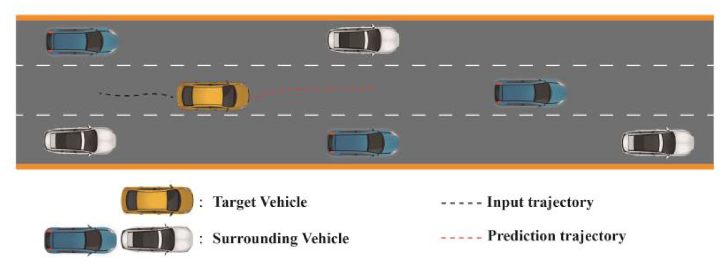
We consider trajectory prediction as a time series forecasting problem. However, based on the time dimension, we have also considered the space dimension here, so the input data are spatial–temporal, which have a data shape of $\left(node,time,dim\right)$. In addition, Figure 3 shows the specific research scenario. We considered the impact of vehicles in eight directions around the target vehicle.

In this paper, the vehicle trajectory prediction problem is expressed as predicting the future trajectory of the target vehicle based on the observed historical trajectory of the target vehicle and its surrounding vehicles. At the time step $t$, the spatial–temporal historical state of the region can be described as $S^t=\left\{s_0^t,s_1^t,\dots ,s_N^t\right\}$, it representing the state of a total of $N$ vehicles at the current moment. The state $s_i^t$ of the vehicle $i$ includes the coordinates $x_i^t$ and $y_i^t$, relative to the origin. Here, the superscript represents the time step, and the subscript represents the car number.

If considering the time dimension, the input can be represented as $x\in R^{N\times T\times 2}$, where $N$ represents the number of vehicles, $T$ represents the historical time step length, and 2 represents the three variables $x_i^t$ and $y_i^t$.

For the output, $H$ was used to represent the predicted horizons. The future trajectory of the target vehicle can be represented as $P_{target}=\left\{p_{target}^{T+1},p_{target}^{T+2},\cdots ,p_{target}^{T+H}\right\}$, where $p_{target}^{T+h}$ represents the coordinates at a time point $h$, so $P_{target}\in R^{2\times H}$, and 2 represents the two variables $x_{target}$, $y_{target}$.

To sum up, the trajectory prediction problem in this article can be represented as Formula (4):

$$P_{target}=F\left(\theta ,x\in R^{N\times T\times 2}\right),$$

(4)

where $F$ represents the proposed model, and $\theta$ is the parameters of the model, which can be continuously optimized through the gradient descent algorithm.

4.2. Model Structure

The overall model structure is shown in Figure 4. It is an end-to-end model with spatial–temporal data as input and a matrix of 2-variate time series as output. In addition, the feature extraction structure is based on the CNNs, SENet, and Vit.

In the first stage of processing spatial–temporal data, we employ 2D convolutional kernels to extract stereoscopic features from different spatial–temporal segments. This process involves increasing the number of channels progressively, enabling the model to learn diverse semantic features that capture both local and global patterns within the data. By stacking multiple convolutional network layers, the receptive fields of the extracted features expand, leading to more abstract representations. These higher-level features represent complex spatial–temporal blocked structures that encapsulate intricate relationships between temporal sequences and spatial distributions. To enhance the expressiveness of these features, we integrate SENet for channel-wise feature fusion. This mechanism allows the model to recalibrate channel-wise feature responses by modeling interdependencies between channels, thereby emphasizing informative features and suppressing less useful ones. Additionally, for intra-channel feature fusion, we utilize Vision Transformers (Vit) to facilitate feature exchange across different parts of a single channel. This approach ensures comprehensive coupling of spatial–temporal features, creating a robust representation that integrates both global and local information.

Following the feature extraction backbone, the next step is to prepare these fused features for input into a Multi-Layer Perceptron (MLP) to feature space mapping and function fitting. To achieve this, we flatten the spatial–temporal fused features into a one-dimensional vector. This transformation simplifies the feature representation while preserving the rich information captured during the earlier stages of processing. The flattened features are then passed through an MLP, which performs nonlinear transformations to map the input features into a higher-dimensional space. This process enables the model to learn complex mappings between the input spatial–temporal data and the desired output. Ultimately, the MLP outputs a future time series matrix, which represents the predicted evolution of spatial–temporal patterns over time. This architecture not only captures the inherent complexity of spatial–temporal data but also provides a flexible framework for forecasting and analysis in various domains, such as weather prediction, traffic flow estimation, and video understanding.

4.3. Stereoscopic Feature Extraction Module

For spatial–temporal data, the spatial dimension is the number of nodes (which can be viewed as the number of channels of image data), the temporal dimension, and the feature dimension, which can be viewed as a time series matrix.

In Figure 5, we show how 2D convolutional kernels extract the stereoscopic features of the spatial–temporal segment. On the one hand, each convolutional kernel in 2D convolutional can extract features from many nodes at the same time. On the other hand, the convolutional kernel within the time series matrix of each node with the shape (time, dim) can extract features from both the temporal dimension and the feature dimension, thereby handling the associations between different variables in multivariate time series and aligning different variables. Therefore, 2D convolutional kernels can be utilized to extract stereoscopic features from the same spatial–temporal segment.

The calculation formula for each convolutional kernel $n$ is as follows (5). Kernel size is $k\times k$, $W$ is the kernel weight, and $X^{t\times d}$ is an input with time length $t$ and variable number $d$. The kernel performs the same operation on each node and then obtains the features of all nodes within time $t$ and dimension $d$. As the convolution kernel continuously slides in two directions in $T\times D$, it extracts features between different time and feature dimensions in all regions, and then obtains a feature map, that is, a channel. Each value of each two-dimensional feature map channel is calculated by a convolution kernel, as shown in Formula (6), where $act$ is nonlinear activation function, and $T^{\prime }\times D^{\prime }$ is the shape of the feature map.

$$kernel\_out=act\left({\displaystyle \sum _{n=1}^{Node}{W}_n^{k\times k}}{X}^{t\times d}\right)$$

(5)

$$Feature\_map\in R^{T^{\prime }\times D^{\prime }}=concat\left({\displaystyle \sum _{i=0}^{T^{\prime }}{\displaystyle \sum _{j=0}^{D^{\prime }}kernel\_ou{t}_{ij}}}\right)$$

(6)

4.4. Loss Function

RMSE (root mean squared error) using squared penalization terms can effectively narrow the error between predicted and true values. Therefore, this paper uses RMSE loss functions. The formula for RMSE is shown in Formula (7).

$$los{s}_{RMSE}={\displaystyle \frac{{\displaystyle \sum _{h\in \left[1,H\right]}\sqrt{{\left(x_{real}^{T+h}-x_{pred}^{T+h}\right)}^2+{\left(y_{real}^{T+h}-y_{pred}^{T+h}\right)}^2}}}{H}},$$

(7)

where $los{s}_{RMSE}$ has the physical meaning of the accumulated error between the predicted positions in the prediction time domain and the actual positions. $H$ is maximum prediction horizon.

For the input, we fill the data with 0 if there is no vehicle to ensure the matching of tensor dimensions and finally obtain the input tensor with a shape of $\left(node,time,dim\right)$.

We use some convolutional neural network layers to extract stereoscopic spatial–temporal block features and set a feasible number of output channels. Therefore, we can obtain some feature map tensors with a shape of $\left(H,W\right)$, which is derived from the shape of $\left(time,dim\right)$. For each feature map, we divide it into some patches, then convert each patch into sequential tokens and use Vit to extract and fusion features from different spatial–temporal blocks. For all feature maps, we globally pool them into a scalar and finally form a one-dimensional tensor. Then, we use a dense attention mechanism to fuse features between different feature maps, which are derived from SENet. For fully connected layer MLP, we output the reshape as the shape of the label, with a loss function of a RMSE.

5. Experiments and Results

5.1. Datasets and Setting

5.1.1. Datasets Introduction

The HighD Dataset is a large-scale natural vehicle trajectory dataset from German highways, including 11.5 h of measurements from six locations and 110,000 vehicles. The total traveled distance of the measured vehicles is 45,000 km, with a positioning error typically less than ten centimeters using State-of-the-Art computer vision algorithms. Therefore, it can be used for trajectory prediction research [47].

The HighD Dataset coordinate system is as shown in Figure 6, where the horizontal axis to the right represents the positive direction of $x$, and the vertical axis downward represents the positive direction of $y$, with the origin at the top left corner. In the HighD Dataset, the FPS is 25, while some of the literature has changed it to 5 FPS. This can reduce the tensor dimension of the labels $p_{target}^{\left(T,T+h\right)}$ and improve the prediction effect. In this paper, 75 historical time steps (3 s) are used as input, and the output is the future two-dimensional trajectory coordinates of the target vehicle.

We conducted experiments using publicly available NGSIM datasets I-80 and US-101, which are in show Figure 7. Each sub-dataset consists of real highway traffic trajectories captured at a frequency of 10 Hz within 45 min. We divided the dataset into a training set and a testing set. We used one-quarter of the trajectories from each of the three subsets of the US-101 and I-80 datasets in the test set. We divide the trajectory into 8 s segments, Where we use a 3 s trajectory history and a 5 s prediction range. These 8 s segments are sampled at a 10 Hz dataset sampling rate.

5.1.2. Datasets Preprocessing

Based on the problem definition and the data format of the HighD Dataset and NGSIM, we create the corresponding samples here. As it needs to consider spatial features, we select a central vehicle (target vehicle) and assume that its movement is influenced by vehicles in the surrounding eight directions, such as front, back, left, right, and the four corners. We padd the data with 0 if no vehicle is present there. We select the $x$ coordinate and the $y$ coordinate time series of each vehicle as features. For each vehicle in the study region (a total of nine vehicles), we perform min–max normalization on each feature along the time dimension. The formula for min–max normalization is as follows (Formula (8)):

$$x^{\prime }={\displaystyle \frac{x-X_{\min }}{X_{\max }-X_{\min }}},$$

(8)

where $X_{\max }$ and $X_{\min }$ represent the maximum and minimum values in the feature, $x$ represents the original value, and $x^{\prime }$ represents the normalized value. Finally, we use 80% of the samples for training and 20% for testing with two datasets. In addition, we calculate the error metrics after normalizing the predicted values.

5.2. Baseline Models

The baselines models are as follows. These models are all from the latest work in recent years. The summary of the baseline models is listed below.

1. CS-LSTM: A Convolutional Social Pooling model was proposed by Deo [48]. This model integrates long short-term memory networks (LSTM) with convolutional neural networks (CNN) to capture interactions among individuals.

2. NLS-LSTM: A Non-local Social Pooling model introduced by Messaoud [30]. This model extends the idea of social pooling by incorporating non-local dependencies to better understand the context and interactions within a scene.

3. I2T: An intent-based model developed by Zhou [47]. This model focuses on understanding the intentions behind actions or movements, which can be crucial for predicting future behavior accurately.

4. MHA-LSTM: An LSTM model enhanced with Multi-Head Attention mechanism proposed by Messaoud [49]. The addition of multi-head attention allows the model to focus on different parts of the input sequence simultaneously, improving its ability to handle complex patterns.

5. MS-STGCN: A Multi-Scale Spatial–Temporal Graph Convolutional Network was created by Tang [50]. This model captures both spatial and temporal dynamics at multiple scales, making it particularly useful for tasks involving sequences of actions over time.

6. EA-NET: The Environment-Attention based model was designed by Cai [44] in 2021. This model considers the environment’s influence on behavior or events, making it suitable for scenarios where environmental factors play a significant role.

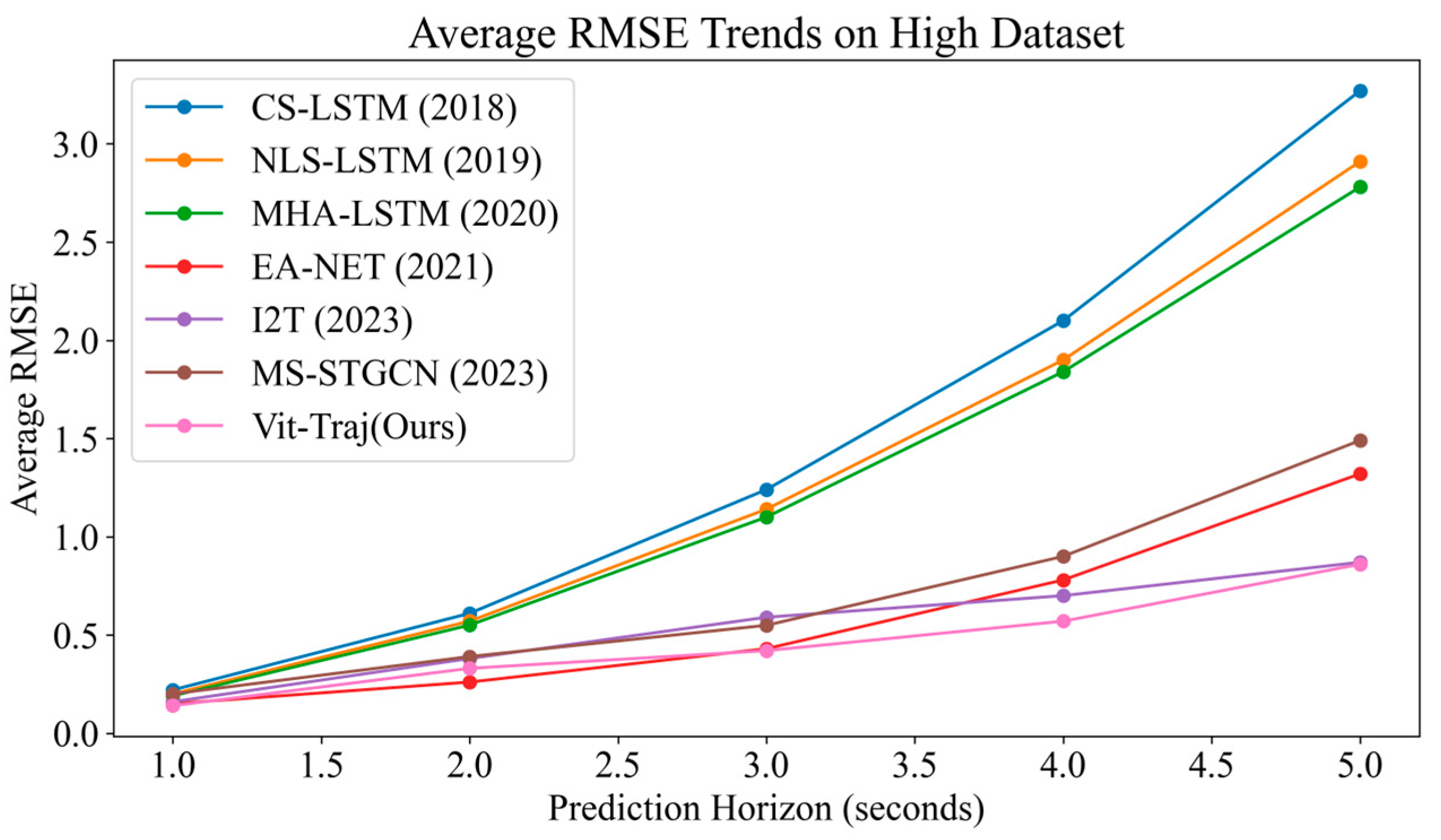
5.3. Comparison of Results on HighD

We use 80% of the data for model training and 20% for model testing. We infer future trajectories for each of the 20% samples using the model and then perform denormalization. The input time step is fixed at 3 s, and the output horizon ranges from 1 s to 5 s. So, the tensor shape of the input samples is $\left(BatchSize,9,75,2\right)$, where 9 represents the nine vehicles in the research scenario, 75 represents a total of 75 time points for the past 3 s (at 25 Hz), and 2 represents the coordinates $x,y$ of the corresponding vehicle. The output tensor form is $\left(BatchSize,T^{\prime },2\right)$, where $T^{\prime }$ can be represented as 25, 50, 75, 100, 125.

Table 2. Average RMSE of models on HighD Dataset (25 HZ).

Prediction Horizons (s)	1 s	2 s	3 s	4 s	5 s
CS-LSTM (2018)	0.22	0.61	1.24	2.10	3.27
NLS-LSTM (2019)	0.20	0.57	1.14	1.90	2.91
MHA-LSTM (2020)	0.19	0.55	1.10	1.84	2.78
EA-NET (2021)	0.15	0.26	0.43	0.78	1.32
I2T (2024)	0.16	0.38	0.59	0.70	0.87
MS-STGCN (2023)	0.20	0.39	0.549	0.90	1.49
Vit-Traj	0.14	0.33	0.42	0.57	0.86

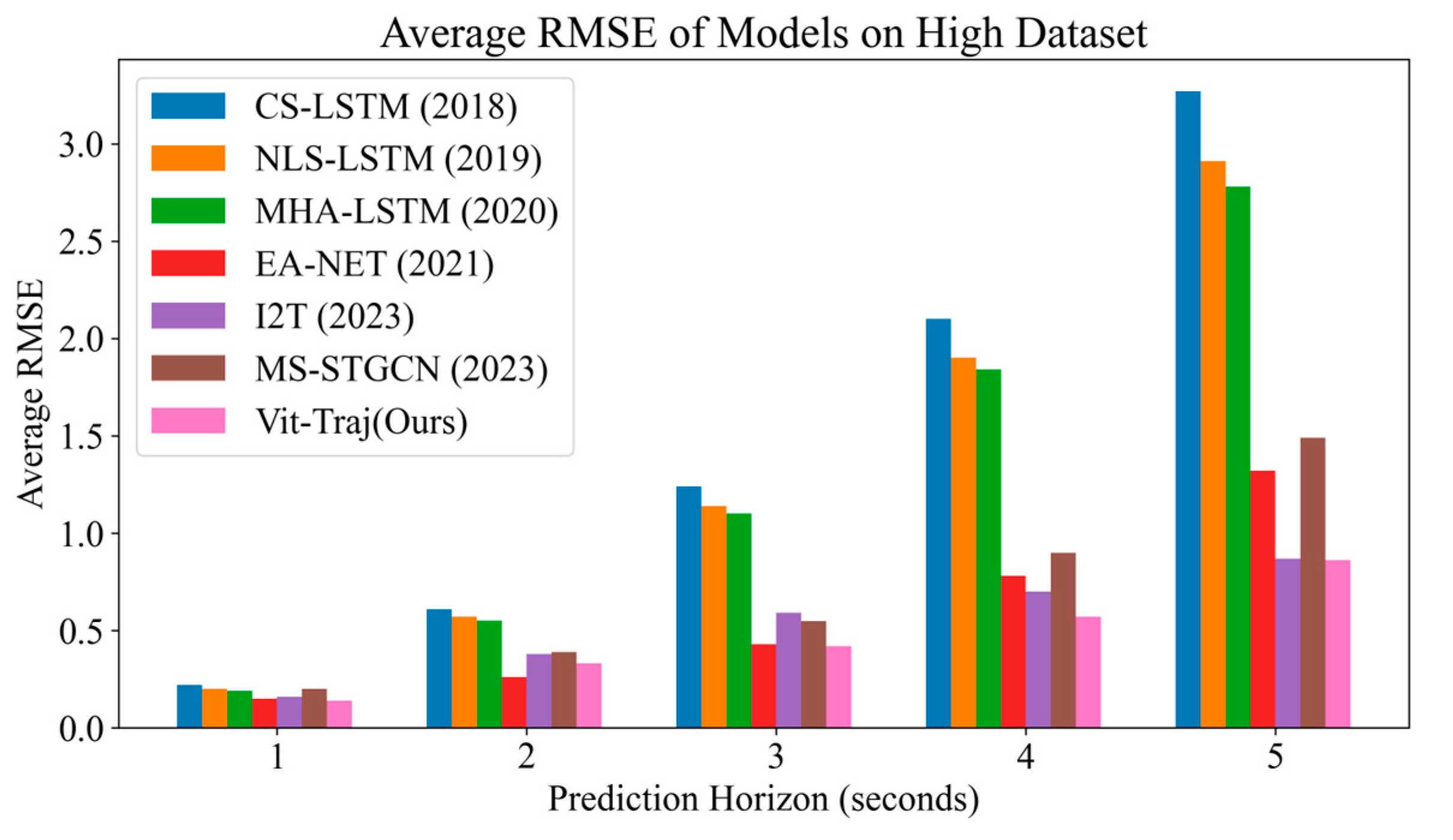
The bold indicates that our model experiments worked best.

shows the results of the proposed model. This table presents the performance of different models across various prediction horizons, ranging from 1 s to 5 s. The metric used is RMSE, where a small RMSE value indicates better predictive performance. In addition, all metrics were calculated at a sampling frequency of 25 Hz.

From Table 2, it can be seen that our model has achieved the best predictive performance compared to existing works. Compared to the GCN based model, our model performs better. The Vit-Traj demonstrates superior performance across all prediction horizons compared to the baseline models, showcasing a significant enhancement in predictive accuracy. Notably, at the shortest prediction horizon of 1 s, Vit-Traj achieves an error value of 0.14, representing a 6.7% reduction from the closest competitor, EA-NET. As the prediction horizon extends, Vit-Traj maintains its lead with relatively stable improvements over longer durations. For instance, at a 5 s prediction horizon, Vit-Traj’s error value stands at 0.86, reflecting a 36.7% improvement over EA-NET’s error of 1.32 and a remarkable 73.7% reduction compared to the baseline CS-LSTM model, which has an error of 3.27 at the same interval. This consistent outperformance underscores the robustness and efficiency of the Vit-Traj architecture in handling complex temporal dynamics.

Figure 8’s bar chart presents the average root mean square error (RMSE) of various models on a HighD dataset, with prediction horizon ranging from 1 to 5 s. It can be observed that the performance of the models deteriorates as the prediction horizon increases, with higher RMSE values indicating lower accuracy. Among the models, Vit-Traj (ours) consistently exhibits the lowest RMSE values across all prediction horizons, suggesting superior performance compared to others. In contrast, CS-LSTM displays the highest RMSE values, indicating its inferior effectiveness.

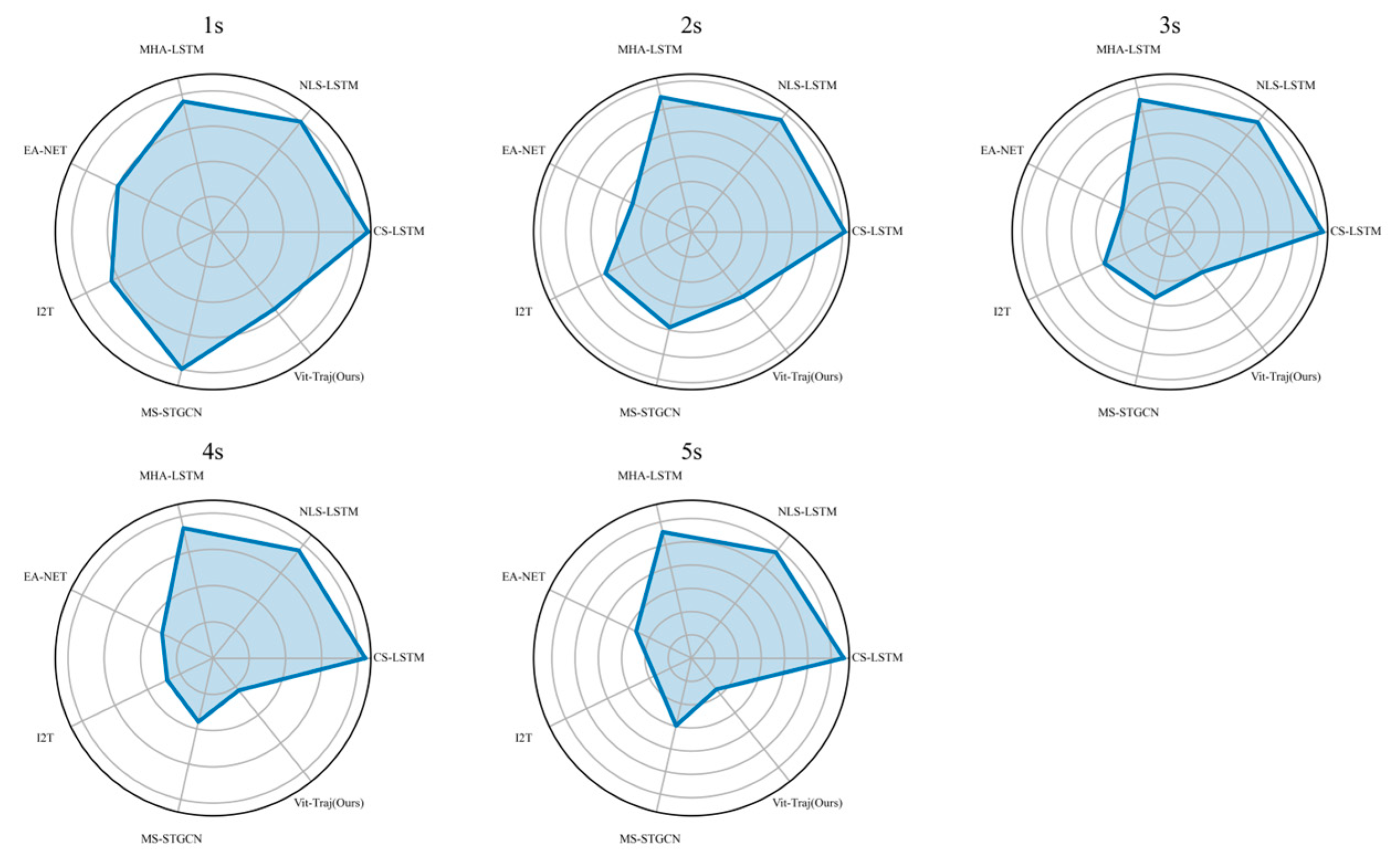
Figure 9 shows the RMSE radar graph of different models with different prediction steps, which provides a more intuitive view of the errors of different models. In the radar images with prediction steps of 1, 3, 4, and 5, our model achieved the lowest RMSE.

Figure 9 presents the average RMSE trends for various models on a HighD dataset, with the x-axis representing the prediction horizon in seconds and the y-axis showing the RMSE values. From the chart, it is evident that the Vit-Traj model (represented by the pink line) consistently outperforms other models, such as CS-LSTM, NLS-LSTM, MHA-LSTM, EA-NET, I2T, MS-STGCN, and others. The Vit-Traj model exhibits lower RMSE values across all prediction horizons compared to its counterparts. The performance improvement of the Vit-Traj model can be attributed to its ability to effectively capture complex patterns and dependencies within the data, which results in more accurate predictions. This superior performance suggests that the Vit-Traj model might be better suited for tasks involving HighD datasets in which precision and accuracy are crucial factors.

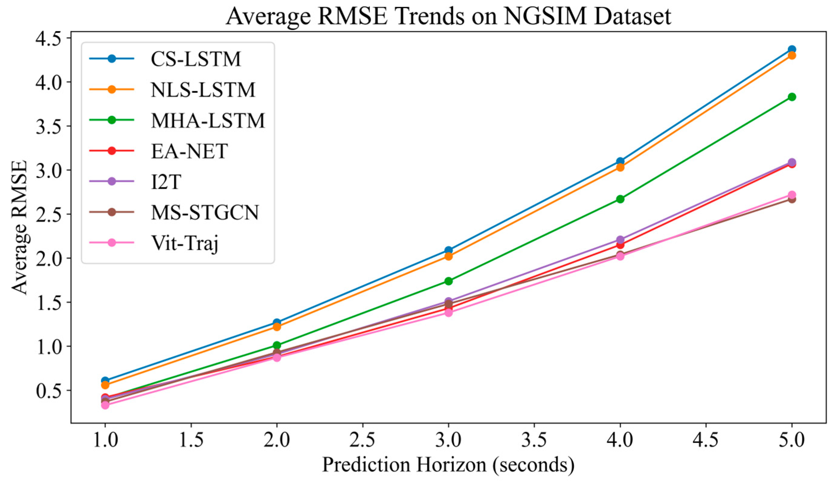
5.4. Comparison of Results on NGSIM

We also use 80% of the data for model training and 20% for model testing. The input time step is fixed at 3 s, and the output horizon ranges from 1 s to 5 s. But because the frequency if different, the tensor shape of the input samples is $\left(BatchSize,9,30,2\right)$, where 9 represents the nine vehicles, 30 represents a total of 30 time points for the past 3 s (at 10 Hz), and 2 represents the coordinates $x,y$ of the corresponding vehicle. The output tensor form is $\left(BatchSize,T^{\prime },2\right)$, where $T^{\prime }$ can be represented as 10, 20, 30, 40, 50.

Table 3. Average RMSE of models on the Ngsim Dataset (10 Hz).

Prediction Horizons (s)	1 s	2 s	3 s	4 s	5 s
CS-LSTM (2018)	0.61	1.27	2.09	3.10	4.37
NLS-LSTM (2019)	0.56	1.22	2.02	3.03	4.30
MHA-LSTM (2020)	0.41	1.01	1.74	2.67	3.83
EA-NET (2021)	0.42	0.88	1.43	2.15	3.07
I2T (2024)	0.40	0.91	1.51	2.21	3.09
MS-STGCN (2023)	0.37	0.93	1.48	2.04	2.67
Vit-Traj (ours)	0.33	0.87	1.38	2.02	2.72

The bold indicates that our model experiments worked best.

compares the average root mean squared error (RMSE) for different models predicting vehicle trajectories on the NGSIM dataset over various prediction horizons from 1 to 5 s, and its sample frequency is 10 Hz. The summary of the model performance are as follows. CS-LSTM shows a steady increase in error as the prediction horizon increases, with an RMSE of 0.61 at 1 s and rising to 4.37 at 5 s. NLS-LSTM has a slight improvement over CS-LSTM, with lower RMSE values across all horizons, such as 0.56 at 1 s and 4.30 at 5 s. MHA-LSTM performs significantly better than the previous two, with RMSE values like 0.41 at 1 s and 3.83 at 5 s. EA-NET is an another improvement, with RMSE values such as 0.42 at 1 s and 3.07 at 5 s. I2T model has a competitive performance with EA-NET, with RMSE values close to EA-NET but slightly higher at longer horizons, like 0.40 at 1 s and 3.09 at 5 s. The MS-STGCN model stands out with relatively low RMSE values, which are particularly noticeable at the longer horizons, such as 0.37 at 1 s and 2.67 at 5 s. The Vit-Traj model (ours) appears to have the best performance overall, showing the lowest RMSE values across all prediction horizons, ranging from 0.33 at 1 s to 2.72 at 5 s.

In summary, Vit-Traj is performing the best among the listed models, suggesting that it is more accurate in predicting future trajectories on the NGSIM dataset compared to the other models mentioned.

Figure 10 displays the average RMSE of various models on the NGSIM dataset, showcasing the RMSE metrics of models. These models have been evaluated within a prediction range of 1 to 5 s. As the prediction range increases, the RMSE of most models also increases, indicating an increased difficulty in making accurate predictions over longer periods of time. However, at many points, the Vit-Traj model consistently exhibited the lowest RMSE, indicating outstanding performance in this task. From Figure 11 and Figure 12, it can be seen that our model achieved good accuracy at step sizes of 1, 2, 3, and 4. However, its performance was inferior to MS-TGCN at a prediction step size of 5, which may be due to MS-TGCN, considering multiple scales. Overall, although our proposed spatial–temporal feature fusion model did not specifically process features from both temporal and spatial perspectives, the results show that the spatial–temporal mixer has a very significant effect.

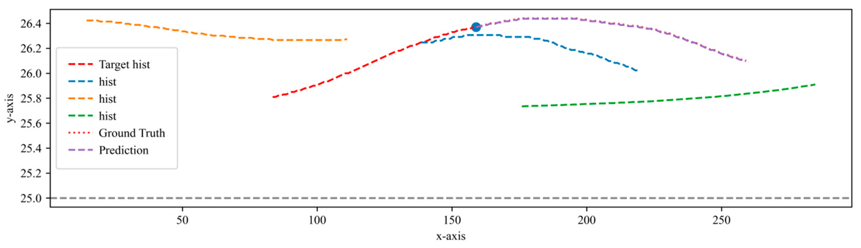
5.5. Spatial–Temporal Prediction Results

To qualitatively evaluate the performance of the model, we visualize the predicted results as shown in Figure 13. This graph not only displays the historical trajectories of surrounding vehicles and target vehicles but also shows the future trajectory of the target vehicle and its actual future trajectory. The corresponding horizon is 75. It is evident from Figure 14 that our model performs well in predicting future trajectories for different traffic flow densities.

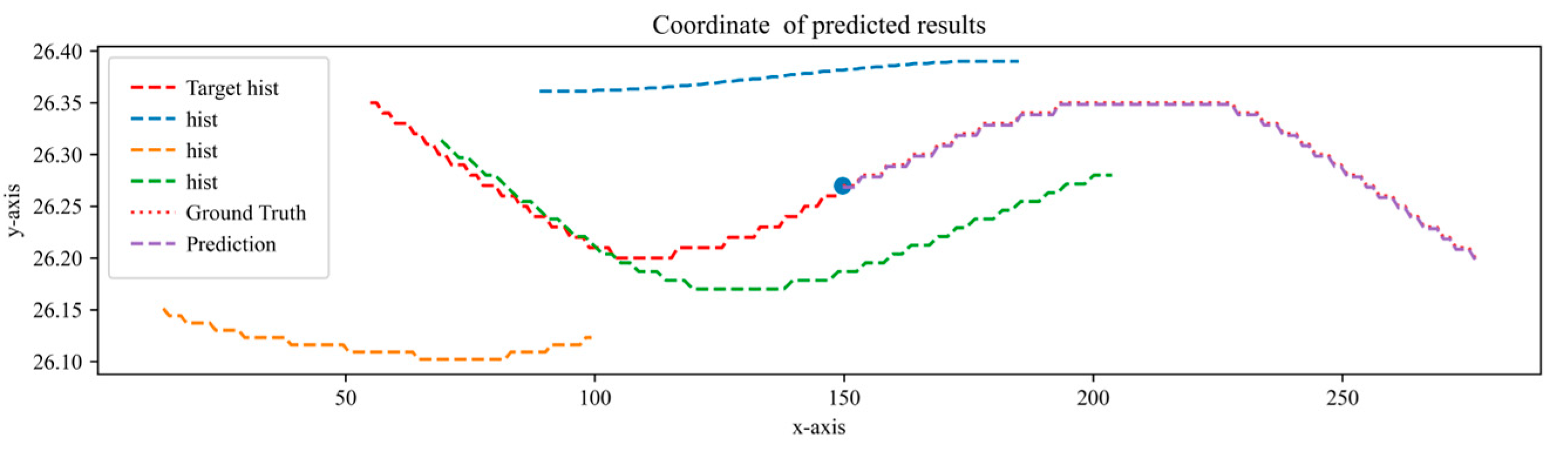
Figure 15 shows a vehicle sample in the NGSIM dataset, displaying the historical trajectories of the target vehicle and surrounding vehicles. Based on these spatial–temporal trajectories, the future trajectory of the target vehicle is predicted. The figure shows the predicted trajectory and the true trajectory, and it can be observed that the predicted values almost coincide with the true values. The model can not only predict the straight trajectory, but also the lane changing trajectory.

5.6. Ablation Experiment

Due to the use of a combination of SENet and Vit for spatial–temporal feature extraction and fusion, we will now demonstrate the results of the experiments conducted, in which we used only one spatial–temporal fusion method to explore the performance of both modules. All experiments were tested on the HighD dataset with a prediction horizon size of 1–5 s.

(a)

Only Vision Transformer

We removed the SENet residual branch from the model for experimentation, while keeping all other experimental parameters consistent with the original experiment and only modifying the necessary tensor transformation network layers.

(b)

Only SENet

We excludede the mainstream Vit in the model and only retained the channel spatial–temporal mixer SENet flow for experimentation.

From

Table 4. Average RMSE comparison of Vit stream/SENet stream and Overall model.

Horizons	Overall Model	Only Vision Transformer	Only SENet
1 s	0.140	0.15	0.15
2 s	0.330	0.35	0.34
3 s	0.420	0.44	0.45
4 s	0.570	0.59	0.61
5 s	0.860	0.88	0.90

and Figure 16, it can be seen that the results of the ablation experiment show that the performance of the Vit stream and the SENet stream is significantly lower than that of the complete model, and the effectiveness of the SENet stream alone is also lower than that of the Vit stream alone.

This indicates that SENet uses global pooling of feature maps to fuse relationships between different feature maps. This has drawbacks, mainly due to the loss of important information caused by global pooling. The Vit stream fuses different spatial–temporal blocks of each feature map, avoiding the drawbacks of global pooling. Fortunately, the proposed Vit-Traj model integrates these two advantages, further improving predictive performance.

6. Conclusions

In this paper, the vision Transformer is applied to vehicle trajectory prediction of spatiotemporal data. The proposed Vit-Traj model significantly improves the prediction accuracy through spatiotemporal feature coupling, which may be an initial attempt. The model can simultaneously extract coupled features of time and space, making time and space compatible with each other rather than separated. Experiments on the HighD dataset and NGSIM dataset show that, compared to State-of-the-Art models, the proposed model exhibits better performance, proving the feasibility of using CNN and ViT for modeling spatial–temporal data and indicating that Vit is a good feature extraction structure for spatial–temporal data. In the future, its applicability to other spatiotemporal data scenarios can be further studied.