Optimization of EMS Station Layout Based on a New Decision Support Framework

Abstract

The layout of emergency medical services (EMS) is of vital importance. A well-planned layout significantly impacts the timeliness of response and operational efficiency, which are crucial for saving lives and mitigating injury severity. This paper presents a novel decision support framework for optimizing EMS station layout. Employing the k-means clustering algorithm in combination with the elbow method and silhouette coefficient method, we conduct a clustering analysis on a patient call record dataset. Comprising 166,161 emergency center call records in the Shanghai area over one year, this dataset serves as the basis for our analysis. The analysis results are applied to determine EMS station locations, with the average ambulance patient pickup time as the evaluation criterion. A simulation model is utilized to validate the effectiveness and reliability of the decision-making framework. An experimental analysis reveals that compared with the existing EMS station layout, the proposed framework reduces the average patient pickup time from 11.033 min to 9.661 min, marking a 12.441% decrease. Furthermore, a robustness test of the proposed scheme is carried out. The results indicate that even when some first-aid sites fail, the average response time can still be effectively controlled within 9.9 min. Through this robustness analysis, the effectiveness and reliability of the decision framework are demonstrated, offering more efficient and reliable support for the EMS system.

1. Introduction

In modern society, EMS are crucial for people’s safety and health. The pre-hospital emergency system bears the responsibilities of daily medical emergencies, emergency response to public emergencies, and major event support, which are related to people’s well-being and urban safety. Today, with the intensification of population aging, the transformation of public health awareness, and the increasing dependence on public resources, pre-hospital emergency services are showing a sustained growth trend. Ambulances are used as the main means of transportation to medical institutions, and research has shown a strong correlation between transportation time and patient survival outcomes [1]. This highlights the importance of fast and efficient ambulance operations.

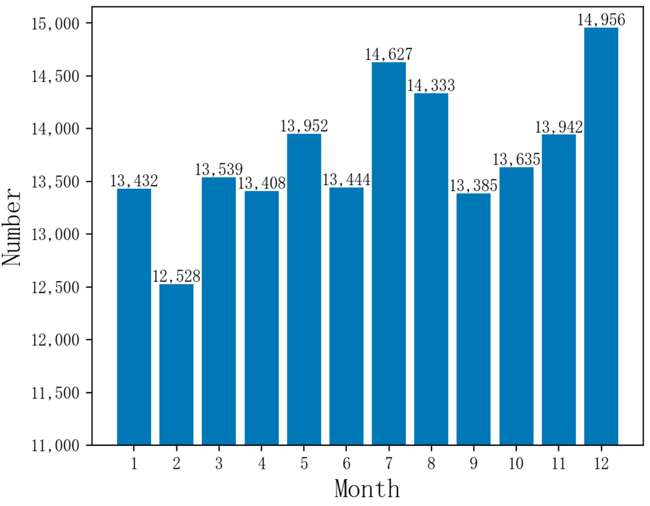
Currently, China has over 300 prefecture-level and over 2000 county-level cities with urban EMS centers, creating a second or third-tier urban EMS network for emergency services and public health emergencies. Shanghai’s pre-hospital EMS system leads the nation in organizational scale, resource number, service capacity, and total volume. It has achieved an average response time of under 12 min based on a year’s dataset of emergency calls, which is a top-tier response time in China. However, there is still room for improvement compared to the world’s advanced cities with a response time of within 10 min [1,2]. Figure 1 reveals that Shanghai’s monthly emergency call volume surpasses 10,000, peaking near 15,000, highlighting the need for well-prepared EMS centers and medical resources.

Figure 1. Monthly emergency call data volume in Shanghai.

Although increasing the number of emergency stations and ambulances may appear to enhance the capacity of emergency services on the surface, in reality, this approach not only increases the financial burden but also cannot completely solve various problems encountered in emergency services. Therefore, by optimizing the layout of existing emergency stations, this article can effectively reduce financial expenditures, improve the overall efficiency of emergency services, and enhance the efficiency and coverage of EMS. Therefore, the reasonable layout of EMS stations is crucial for improving the efficiency and coverage of EMS [3,4].

Related Work

The traditional station selection problem is often based on experience and intuition and lacks scientific validity and accuracy. In tackling this challenge, researchers have conducted an in-depth investigation into three pivotal areas: the strategic layout design and optimization of first aid stations, the enhancement of geospatial distribution through the application of clustering algorithms, and the utilization of simulation techniques to refine these approaches.

Researchers have tried different models and methods to improve the efficiency and coverage of EMS stations. Golabian et al. [5] proposed two location models in combination with a hypercube queuing model to get the location information of the ambulance stations to maximize the de-coverage of the patients, and based on that, they used simulated annealing algorithms and discrete event simulation to solve large-scale problems. Aboueljinane et al. [6] proposed a discrete simulation-based optimization model to find the location of the rescue team and combined it with a simulation to evaluate the final results. Onur et al. [7] proposed a multi-objective mathematical model to solve the field hospital siting problem by combining the Enhanced Two-Step Floating Catchment Area (E2SFCA) method with a travel time-constrained capable p-median model to maximize the minimum reachability and minimum travel time. Akpinar et al. [8] proposed a VIKOR method-based field hospital location model after a possible post-earthquake site selection model, and the most suitable location for the COVID-19 field hospital was determined by a fuzzy Choquet integral multi-criteria decision-making technique. Zhang et al. [9] proposed using a Gaussian two-step moving search method, K-means clustering, and a particle swarm algorithm. They carried out a spatial accessibility and location analysis of emergency sheltering places. The study proved that 10 new emergency shelters can reduce the number of passable blind zones by 43.31%. Hassan et al. [10] determined the location of the new Crown Pneumonia field hospitals by solving a nonlinear binary-constrained model to maximize the number of patients. Grot M [11] proposed a new stochastic, time-varying, mixed integer extended maximum expected coverage siting problem considering ambulance site interdependencies for computational experiments on an existing emergency medical services network structure to optimally locate sites and assign ambulances. The above studies demonstrate that by optimizing various models and methods, the layout of EMS stations can be improved, thereby enhancing the efficiency and coverage of the stations. These models and methods provide a theoretical basis and methodological support for our research.

Clustering algorithms show great potential in optimizing geospatial layout. Wang et al. [12] combined the k-means method with the 2DULVs (Two-dimensional Uncertain Linguistic Variables) - TOPSIS (Tailored to Ideal Solution Similar Ranking Preference Technique)-DDSCCR (Dempster-Shafer Joint Combination Rule) model to screen and evaluate all the areas in the target area for Internet medical companies to establish offline clinics, and finally get the most suitable geographic layout for the establishment of offline clinics. Han et al. [13] utilized the k-means clustering algorithm to analyze the demand spatiotemporal points of the demand for emergency services, and based on the results of data clustering and Gaussian distribution fitting, Monte Carlo simulation of the demand points was carried out. Wang [14] proposed applying a genetic algorithm and k-means clustering algorithm to the problem of selecting the location of the base station, and the k-means algorithm was used to analyze the clustering of the region to get the optimal solution. Luo [15] proposed the use of a k-means algorithm to solve the site planning and region clustering problem of a mobile communication network. Fan [16] proposed the k-means clustering algorithm to reduce the search range of solution space and realize the scientific site selection of emergency rescue organizations. Sonta et al. [17] used a combination of a clustering-based method and genetic algorithm with the goal of reducing energy consumption to obtain a building layout with a 5% reduction in energy consumption after optimization. Lin et al. [18] proposed a new hierarchical clustering framework for the location selection of facilities that can flexibly support a variety of optimization objectives. These studies show the potential of clustering algorithms for application in geospatial layout optimization. The above studies indicate that the application of clustering algorithms offers a valuable approach to site selection, thereby improving the rationality and scientific validity of the process. These studies provide references for us to select and apply clustering algorithms.

Simulation techniques have also been widely used to support layout problem analysis and solutions. Wenya et al. [19] built a system dynamics model of a mass casualty incident (MCI) in Shanghai to improve the efficiency of the MCI rescue by adjusting the size of the MCI, the allocation of the ambulances, the allocation of the emergency medical personnel, and the efficiency of the organization and command. Wu et al. [20] used simulation software to construct agent-based modeling with allocated resources and Monte Carlo methods to simulate stochastic rescue behaviors and applied these to the field of emergency evacuation. Traoré et al. [21] proposed a modeling and simulation framework to support the holistic analysis of healthcare systems by layering the abstraction hierarchy into multiple perspectives and integrating them into a common simulation framework. Nogueira et al. [22] analyzed the emergency medical services in Belo Horizonte, Brazil, using two modeling techniques: optimization modeling and simulation. The optimization model located ambulance bases, assigned them, and simulated the proposed configuration to analyze the dynamic behavior of the system. Oliveira et al. [23] used the evolutionary algorithm NSGA-II to solve the problem of the planning of hospital beds and used discrete event simulation to validate and evaluate the solution. These studies demonstrate how simulation can assist in layout design and optimization, providing a scientific basis for decision-making. Simulation models can replicate real-world scenarios, ensuring the reliability of experimental data and providing robust data support for EMS, thereby accurately assessing the performance of EMS services. These studies provide us with methods and tools to verify the validity of the model.

These areas have provided valuable research directions for solving EMS station optimization problems. These studies collectively demonstrate the effectiveness of combining mathematical models, clustering algorithms, and simulation techniques in optimizing EMS station layouts. The site optimization problem requires a comprehensive consideration of factors such as data reliability and the realism of scenario simulations.

Based on the above analysis, this paper constructs a new decision support framework. In this framework, the k-means clustering algorithm is utilized in conjunction with the elbow method and silhouette coefficient method for clustering analysis of the patient call record dataset. The analysis results are then applied to localize EMS stations, the average time required for ambulances to pick up patients is selected as the evaluation criterion, and the simulation model serves as a validation tool to assess the effectiveness and reliability of the decision framework. During the construction of the simulation model, factors such as patient generation rate, patient injury proportion, traffic conditions, ambient distribution, and patient location were taken into account to ensure the reliability of the model.

Section 1 first introduces the background and research status. Section 2 preprocesses and analyzes the dataset, respectively introducing the algorithms and simulation models used in the framework of this paper. Section 3 conducts four experiments to verify the effectiveness and reliability of the proposed method. Section 4, conclusions and directions for future work are presented.

2. Methods

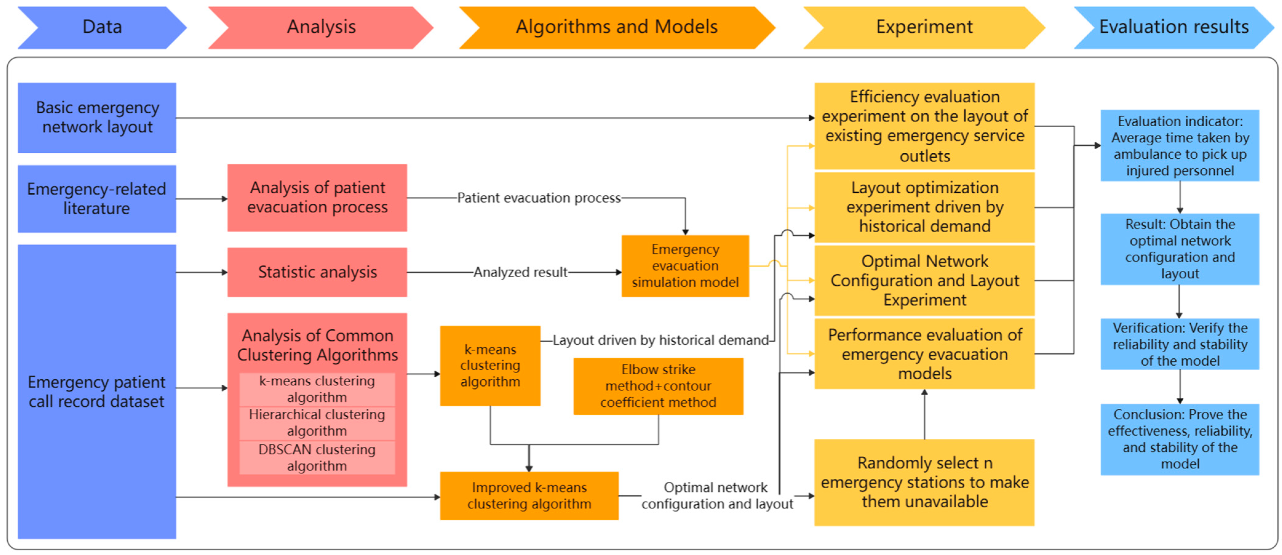
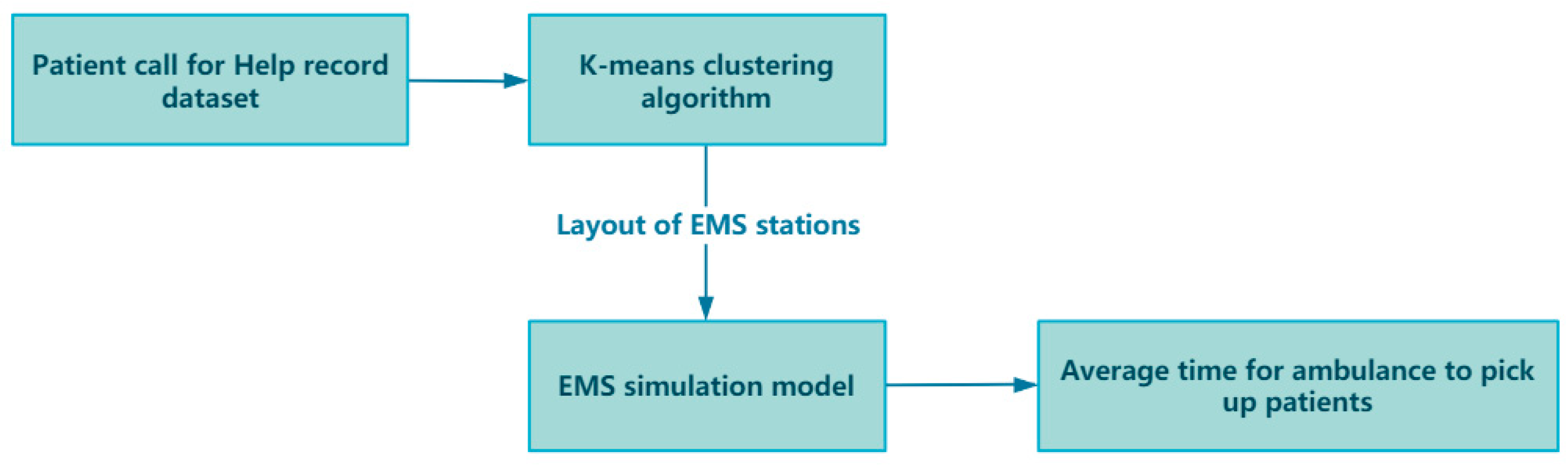
In the framework of this paper, taking Shanghai, China, as an example, the impact of optimizing the layout of EMS stations on the average time for ambulances to pick up patients is studied. The research initiates the preprocessing of a one-year dataset of patient emergency call records from Shanghai, addressing any missing values to ensure data integrity. A thorough analysis of this dataset uncovers critical insights such as the distribution of patient ages, the average hourly call volume, and the proportion of different disease types. These findings lay the groundwork for our simulation models. Next, we apply k-means and improved k-means clustering algorithms to the geographic locations of patient calls to optimize EMS station numbers and layouts across Shanghai’s districts. To validate the algorithm’s effectiveness, we use a simulation model, parameterized by historical data, to ensure model realism and accuracy. The model’s authenticity is verified by comparing real and simulated ambulance response times. Upon validation, the optimized EMS station layouts are subjected to simulation to assess whether they can indeed decrease the average time taken for ambulances to reach patients. Through the simulation and analysis of the simulation model, the effect of the optimized EMS stations in practical applications can be evaluated, and the EMS station layout can be further refined and optimized. Ultimately, the model’s robustness is confirmed, demonstrating that it retains its performance and stability even when confronted with uncertain elements. Figure 2 illustrates the overall framework flowchart of this paper.

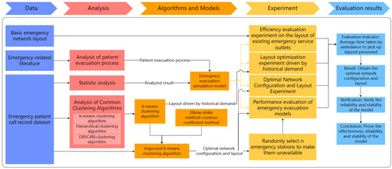
Figure 2. Overall framework flowchart.

2.1. Patient Call for Help Record Dataset

The introduction of historical data helps to identify long-term trends and cyclical patterns in the data. By analyzing historical data, results such as patterns of patient calls for help and the percentage of disease types can be obtained, which is critical for predicting future data points and system behavior and ensures the model’s fidelity and reliability. At the same time, historical data can be used as a benchmark to evaluate the performance of the k-means clustering algorithm and its effectiveness in optimizing the layout of EMS stations, determining whether it can effectively reduce the time for ambulances to arrive at the scene, improve the efficiency and response speed of EMS.

Due to the leading position of Shanghai’s pre-hospital EMSS in China, this paper takes Shanghai as an example to study how to optimize the layout of EMS stations through the framework. The dataset includes one year of patient distress information within the scope of Shanghai. These data are automatically recorded through the system of the Shanghai EMS Center and are processed and used anonymously to ensure the protection of personal privacy. For patient information in the dataset, it mainly includes the following contents:

• Basic patient information, including age and gender;
• Timestamp of the call for help;
• Specific address of the call for help;
• Latitude and longitude of the call for help;
• Time when the ambulance was dispatched;
• Time when the ambulance arrived at the scene;
• Time when the ambulance left the scene;
• Time when the ambulance arrived at the hospital;
• Type of patient injury;
• Hospital to which the patient was sent.

By analyzing the data in the dataset, better data support can be provided for subsequent models, ensuring the adaptability of the algorithm and the authenticity and reliability of the simulation model.

2.2. Data Preprocessing

There are a total of 166,161 pieces of data in the dataset, and the data are automatically recorded through the system of Shanghai EMS Center, so there are only missing values in the data. The task of this chapter is to process the missing values of the data before analysis to ensure its reliability. Common methods to deal with missing values are deletion, filling, interpolation, modeling prediction, and special value filling [24]. Usually, when very few missing values are deleted, no major problems occur. However, deleting a large number of missing values can lead to a large amount of information loss [25]. So, it is also important to handle the missing values in the dataset in a reasonable way. The following are the results of analyzing and processing the attributes in the dataset of this paper.

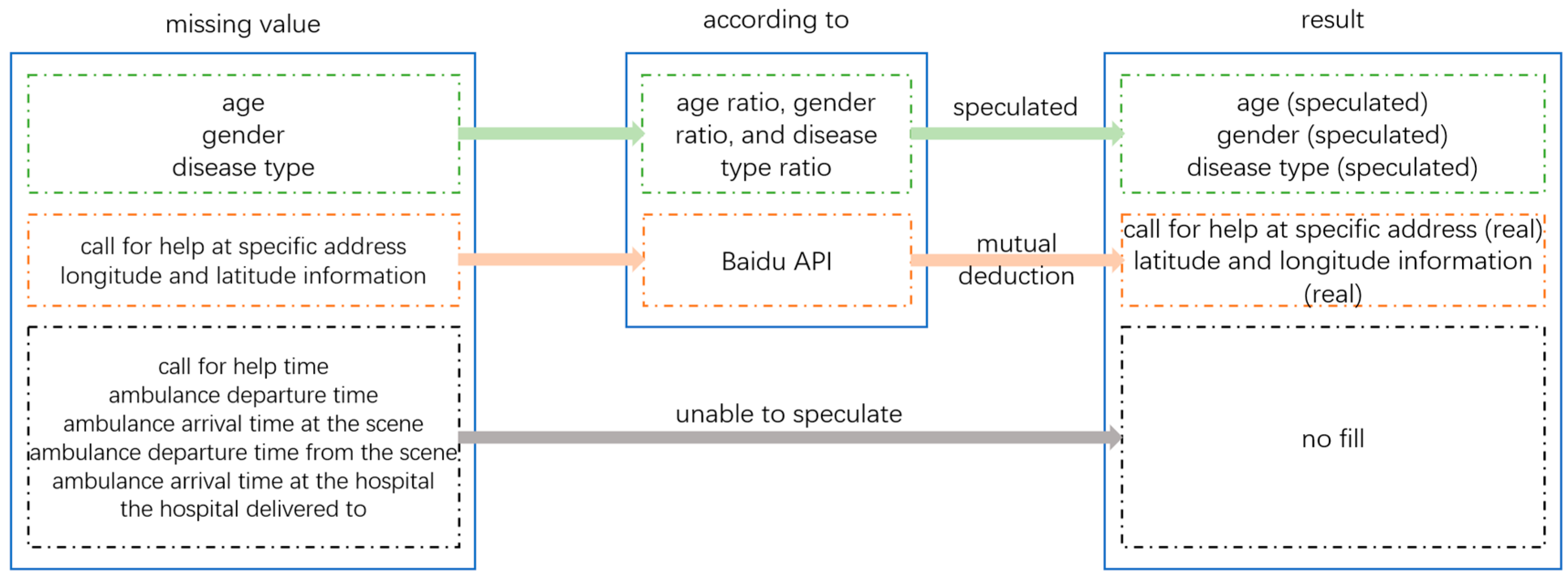
The age, gender, and disease type of patients can be inferred based on existing data ratios and their interrelationships. The specific address and latitude and longitude information of the patient’s distress call can be inferred from each other through Baidu API. Due to the fact that the patient’s call time, ambulance departure time, and arrival time at the scene are related to the actual response time, and the actual data are extremely rare, the inferred data may be inaccurate and affect the actual response time, so there is no need for processing. The three data points of ambulance departure time, arrival time at the hospital, and hospital of delivery have no impact on the construction of the emergency evacuation model, so there is no need to handle their missing values. The logic for handling missing values in the patient distress record dataset is shown in Figure 3, and the analysis and processing of missing values in the patient distress record dataset are shown in Table 1.

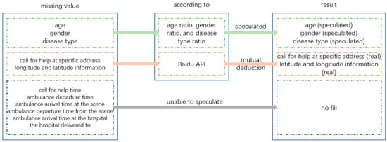
Figure 3. Logic diagram for handling missing values in the dataset.

Table 1. Data statistics and preprocessing results.

	Number of Missing Value Entries	Number of Missing Values After Processing	Percentage After Treatment
Basic patient information	461	0	0.000%
Timestamp of the call for help	12	12	0.007%
Specific address to call for help	254	29	0.017%
Latitude and longitude of the call for help	968	29	0.017%
Time when the ambulance was dispatched	9	9	0.005%
Time when the ambulance arrived at the scene	9	9	0.005%
Time when the ambulance left the scene	12	12	0.007%
Time when the ambulance arrived at the hospital	8822	8822	5.309%
Type of patient injury	46	46	0.028%
Hospital to which the patient was sent	9965	9965	5.997%

2.3. Data Analysis

After data preprocessing, the data in this dataset can be analyzed, and the results of the analysis can be used as input or comparison data for the patient emergency evacuation simulation model, which provides data support for the model and ensures the model’s real reliability.

Analyzing the gender of the patients, we obtain a male–female ratio of 83,248:82,451, which is about 1:1. Analyzing the age of the patients, we obtain the age distribution ratio. As can be seen from the table, with the increase in age, the number of people calling for help increases, among which the 81–90 age group is the largest, accounting for about 30% of the total number of people calling for help. After the age of 90, the number of people calling for help gradually decreases. Table 2 shows the age distribution of patients.

Table 2. Age distribution of patients.

Age Range	Number of People	Percentage
0–5	863	0.519%
6–10	458	0.276%
11–15	525	0.316%
16–20	1740	1.047%
21–25	4486	2.700%
26–30	8504	5.118%
31–35	6054	3.643%
36–40	4600	2.768%
41–45	3998	2.406%
46–50	5184	3.120%
51–55	6725	4.047%
56–60	11,172	6.724%
61–65	11,934	7.182%
66–70	11,292	6.796%
71–75	9159	5.512%
76–80	14,453	8.698%
81–85	25,241	15.191%
86–90	24,527	14.761%
91–95	11,551	6.952%
96–100	3210	1.932%
Over 100	486	0.292%

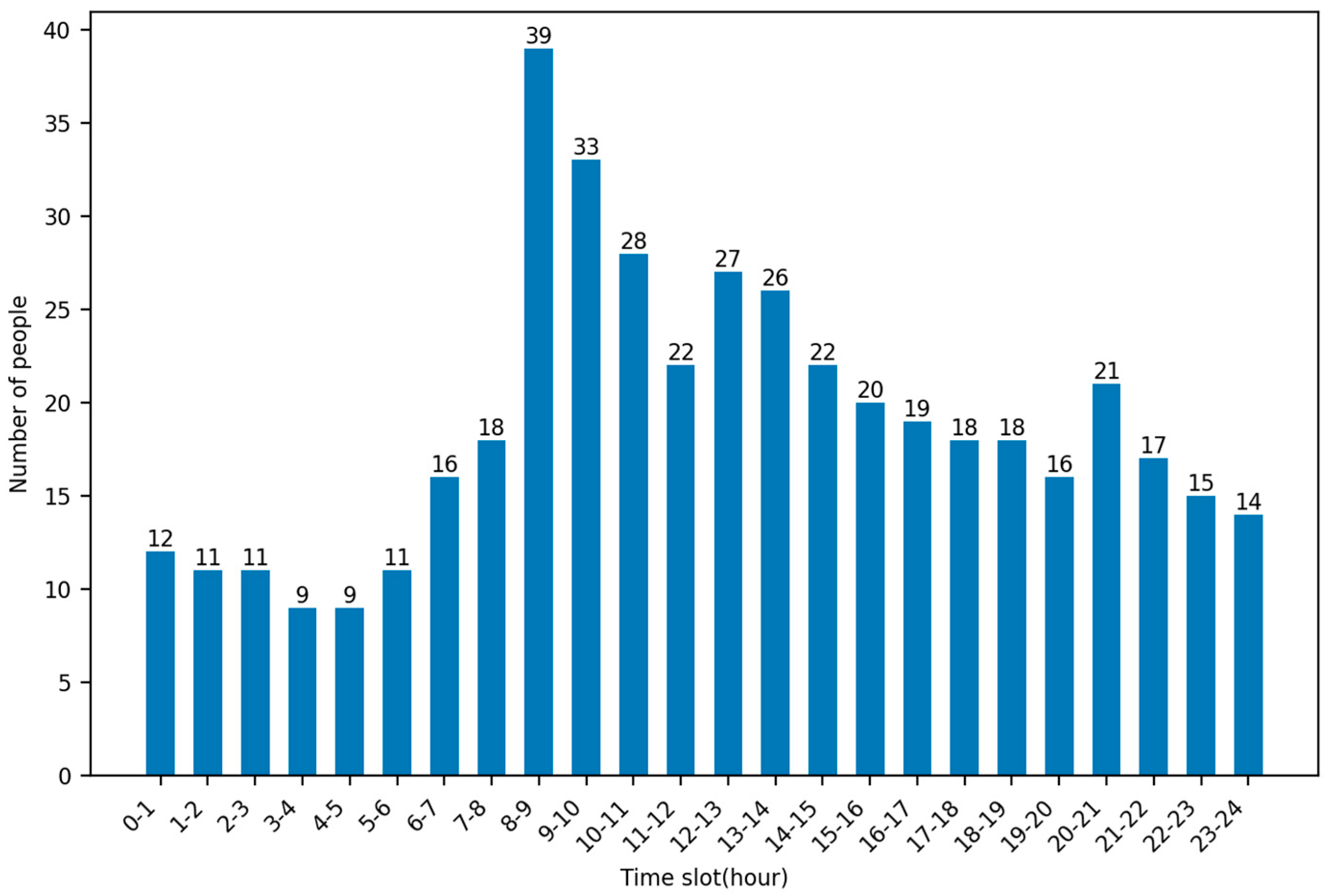
By analyzing the timestamps of patient calls for help in this dataset, it is possible to obtain the rate at which patients are generated at each hour of the day. As can be seen in the figure, the highest average number of calls for help were made at 8–9 pm, up to 39, and the lowest average number of calls for help were made at 3–4 and 4–5 pm, both at 9. Figure 4 shows the average number of people calling for help per hour.

Figure 4. Average number of people calling for help per hour.

Analyzing the ambulance departure time and arrival time at the scene, we obtain the average time for ambulances to pick up the patient, about 10.932, and these data can provide a basis for the realism of the simulation model later. The injury category of the patient is analyzed, and the type and percentage of the patient’s disease can be obtained. Table 3 shows the disease types and percentage of patients.

Table 3. Disease types and percentage of patients.

Type of Disease	Proportions
Pediatric diseases	0.031%
Diseases of obstetrics and gynecology	0.270%
Respiratory diseases	2.886%
Dermatological diseases	11.325%
Mental and behavioral abnormalities	0.635%
Diseases caused by physical and chemical factors	0.876%
Urinary system disease	2.909%
Cerebrovascular disease	3.805%
Endocrine and metabolic diseases	9.923%
Nervous system disease	2.382%
Injury disease	4.545%
Otolaryngology and ophthalmologic diseases	22.187%
Digestive system	0.648%
Blood system diseases	8.885%
Circulatory system	0.322%
Tumor	13.585%
Other diseases	3.016%

2.4. Algorithm

In this section, a method is proposed to reduce the average time for ambulances to pick up patients, specifically by optimizing the layout of EMS stations. Common models for optimizing geospatial layout [10] include traditional models and dynamic location models, whereas traditional models include coverage models and P-median models [4], etc., and dynamic location models have spatial layout site selection and spatial relocation. The difference between the two in the dynamic location model is that in the dynamic layout problem, the decision maker chooses to build a new facility of a certain size at a new candidate point to satisfy the needs of the corresponding moment or time period; whereas in the relocation problem, the decision maker chooses an original supply point and adjusts the size of the service facility to satisfy the needs of the corresponding moment or time period through global scheduling.

This paper aims to relocate EMS stations by analyzing the latitude and longitude of patient calls in a historical dataset. The traditional model needs to abstract the location information of calls for help into demand points, then analyze all demand points, and, finally, obtain the optimal layout information of the EMS station. However, the amount of data in this article reaches hundreds of thousands, and using traditional methods would make the problem more complex. Therefore, this paper chooses to use clustering algorithms to solve the optimization problem of EMS station layout.

Compared with other models, clustering algorithms have a faster calculation speed and can divide patients into several categories by analyzing longitude and latitude information, as well as adjusting the k value to obtain the optimal solution. It has a certain degree of flexibility, so clustering algorithms are used to optimize the location information of EMS stations.

By comparing the performance of common clustering algorithms in the dataset of this paper, this paper chooses to use the k-means clustering algorithm as an analytical tool. By using this algorithm to perform cluster analysis on the patient call data in Shanghai for one year, k clusters can be obtained. The center points of these clusters will represent the ideal location information of EMS stations. At the same time, in the k-means clustering algorithm, choosing the appropriate K value (that is, the number of clusters) is a crucial step that directly affects the quality of the clustering results. Therefore, this article chooses to combine the k-means clustering algorithm with the elbow method and the silhouette coefficient method to find the optimal k value and, finally, obtain the optimal layout of EMS stations.

2.4.1. Comparison of Common Clustering Algorithms

Common clustering algorithms include k-means clustering algorithm [26], DBSCAN and hierarchical clustering algorithm. The k-means clustering algorithm is the most classical and commonly used method; it is a simple and efficient algorithm that is widely used in various fields of scientific research.

A comparative analysis was conducted on these three clustering algorithms using the dataset presented in this article. By observing the average distance between samples and clustering centers under different clustering kernels and the clustering results, the optimal algorithm was selected. Due to DBSCAN being a density-based clustering algorithm, the number of clustering kernels can only be observed by adjusting the neighborhood and core points. The comparison results are shown in Table 4.

Table 4. The average distance between data points and clustering kernels.

	Number of Clustering Kernels
	3	4	5	6	7	8
k-means clustering algorithm	2.835 km	2.432 km	2.125 km	1.924 km	1.755 km	1.654 km
Hierarchical clustering algorithm	2.923 km	2.545 km	2.231 km	2.028 km	1.831 km	1.728 km
DBSCAN clustering algorithm	4.735 km	4.632 km	4.545 km	4.494 km	4.405 km	4.324 km

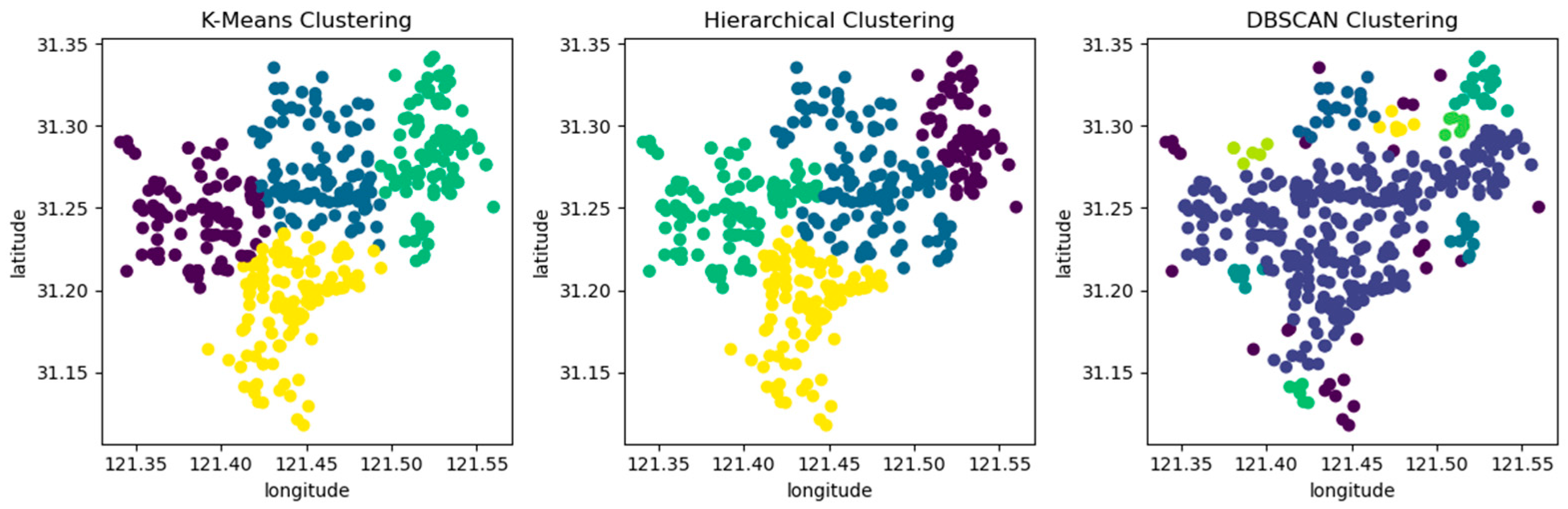
When the clustering kernel is 4, the performance of the three algorithms is shown in Figure 5. The circles in the figure represent the patient’s emergency address, and different colors represent different clusters after clustering.

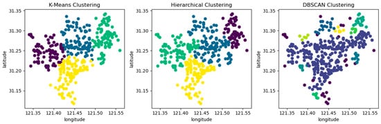
Figure 5. Comparing three clustering algorithms using location information from patient call record dataset.

From Table 4 and Figure 5, it can be seen that the k-means clustering algorithm and hierarchical clustering algorithm perform well, but DBSCAN performs poorly. From Table 4, it can be seen that the DBSCAN clustering algorithm has a longer average distance from the sample to the cluster center under different clustering kernels, which increases the average response time. Moreover, the data in the dataset are evenly distributed, while the DBSCAN clustering algorithm is based on density and is more suitable for datasets with distinct and irregular shapes; for example, as shown in Figure 6. The circles in the figure represent different data points, and different colors represent different clusters.

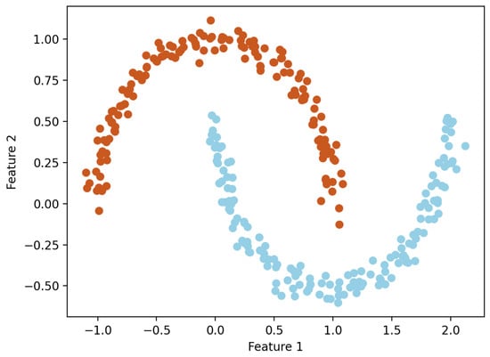
Figure 6. Example diagram of DBSCAN clustering algorithm.

For the k-means clustering algorithm and hierarchical clustering algorithm, hierarchical clustering constructs a tree-like hierarchical structure based on the hierarchical structure of the data. In this process, each step requires distance calculation and merging operations on a large number of data point pairs, which consumes a lot of computing resources and time in the case of large datasets. The time complexity is usually between $O\left(n^{2}logn\right)$ and $O\left(n^3\right)$ ($n$ is the number of data points). The k-means clustering algorithm, on the other hand, does not care about hierarchical structure and only focuses on the distance between data points and cluster centers. Its calculation is relatively simple and only updates k cluster centers in each iteration, resulting in relatively less computational complexity. It has low time complexity and is suitable for large datasets, with a time complexity of $O\left(nkt\right)$ (where $n$ is the number of data points, $k$ is the number of clusters, and $t$ is the number of iterations). Taking the dataset in this article as an example, the running time results of k-means clustering and hierarchical clustering algorithms are shown in Table 5.

Table 5. The running time results of k-means clustering and hierarchical clustering algorithms.

	Algorithm Running Time (Seconds)
k-means clustering algorithm	3.672
Hierarchical clustering algorithm	10.268

According to Table 5, it can be seen that the running time of the k-means clustering algorithm is about 7 s shorter than that of the hierarchical clustering algorithm, which proves that the k-means clustering algorithm performs better than the hierarchical clustering algorithm.

Based on the comparison results of several groups, this paper chooses to use the k-means clustering algorithm to optimize the layout of EMS stations.

2.4.2. K-Means Clustering Algorithm

The k-means clustering algorithm is an unsupervised machine learning algorithm [27] that only requires data without labeling results. It is also an iterative algorithm with low computational complexity, fast speed, and low computational cost, suitable for large-scale datasets. The k-means clustering algorithm can divide samples into several categories based on the intrinsic relationships between data without knowing any sample labels, resulting in high similarity between samples of the same category and low similarity between samples of different categories [28]. The k-means algorithm assigns data points to k cluster centers, each representing an optimized EMS station. This makes the results of optimizing the layout of EMS stations much clearer and more intuitive, which is helpful for practical operation and decision-making.

The specific steps of k-means clustering algorithm:

• Select k cluster centers as the initial cluster centers;
• Calculate the distance between each sample point and each cluster center separately, and assign each sample to the cluster center closest to it;
• Update the cluster center of each cluster, which is defined as the mean of all samples in each dimension within the cluster;
• Compared with the k cluster centers obtained last time, if the cluster centers change, proceed to step 2; otherwise, proceed to step 5;
• When the class center no longer changes, stop iteration and output clustering results.

The parameter k in the k-means algorithm is difficult to determine and usually needs to be specified in advance [29], obtained based on empirical values, or obtained through multiple experiments. For different datasets, there is no reference for the k value. Setting different k values, the number of iterations may be very different, affecting the accuracy of clustering results. Therefore, the first step to obtain good clustering results is to determine the optimal number of clusters [30]. The elbow method and silhouette coefficient are common methods used to determine the optimal number of k clusters in k-means clustering algorithms [31].

The silhouette coefficient can be used to evaluate the clustering results in a way that measures the tightness and separation of the clusters. Silhouette coefficient is a commonly used metric for contour analysis, which takes values ranging from −1 to 1 and indicates the closeness of a sample within the cluster to which it belongs and its separation from other clusters. For each sample in the cluster, their silhouette coefficients are calculated separately; the calculation of silhouette coefficients is shown in Equation (1).

$$S\left(i\right)={\displaystyle \frac{\left(b\left(i\right)-a\left(i\right)\right)}{\max \left(a\left(i\right),b\left(i\right)\right)}},$$

(1)

Here, $a$ represents the degree of dissimilarity within the cluster, which is the average distance between the current sample $i$ and other samples within the cluster; $b$ represents the degree of inter cluster dissimilarity, which is the average distance from the current sample $i$ to the nearest samples in other clusters. The average silhouette coefficient of all samples is called the silhouette coefficient of the clustering result. The closer $S$ is to 1, the closer the sample is within its own cluster, and it is well separated from other clusters. The closer $S$ is to −1, the less tight the sample is within its own cluster, and it overlaps with the boundaries of other clusters. If $S$ is close to 0, it indicates that the sample is near the cluster boundary. When applying the silhouette coefficient analysis method, the number of clusters with the highest silhouette coefficient is usually selected as the optimal number of clusters.

By calculating the silhouette coefficients of the samples, the quality of clustering results can be evaluated, and the optimal number of clusters can be selected based on the silhouette coefficients. The silhouette coefficient analysis method provides a quantitative evaluation method when selecting the number of clusters, which can help us make better clustering decisions.

This method evaluates the quality of the clusters based on the sum of squared errors (SSE) within the clusters. The location where the SSE improvement effect decreases is the elbow, which is usually used to determine the optimal k value. The SSE objective function is as follows.

$$\mathrm{S}\mathrm{S}\mathrm{E}={\sum }_{i=1}^k{\sum }_{x\in {\mathrm{C}}_i}{dist\left(c_i,x\right)}^2,$$

(2)

Among them, $dist$ is the standard Euclidean distance, $k$ is the number of clusters, $x$ is the sample point in cluster $C_i$, and is the centroid of cluster $c_i$. The k-means algorithm uses SSE as the objective function to measure clustering quality. The $SSE\left(i\right)$ of each cluster is equal to the sum of squared distances from each sample point to its class center, and the sum of $SSE\left(i\right)$ of all clusters is the SSE of the clustering result. If members within a class are more compact with each other, the SSE will be smaller. Conversely, if members within a class are more dispersed with each other, the SSE of the class will be larger.

When k is less than the optimal number of clusters, the increase in k will increase the degree of aggregation of each cluster, so the decrease in SSE will be significant. When k reaches the optimal number of clusters, the degree of aggregation obtained by increasing k will rapidly decrease, so the decrease in SSE will sharply decrease and then tend to flatten with the increase of k value. That is to say, the relationship graph between SSE and k is in the shape of an elbow, and the k value corresponding to this elbow is the optimal number of clusters for the data.

Figure 7 shows a line graph using the elbow method, from which it can be seen that the curve starts to flatten out from the point where $k=3$, which leads to the conclusion that $k=3$ is an “elbow point”, i.e., the optimal value of k to look for.

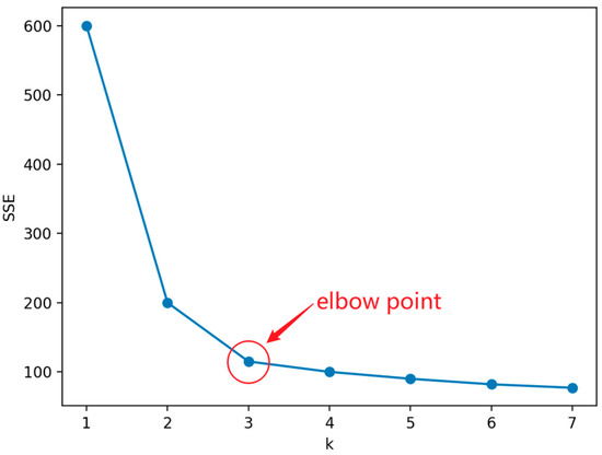
Figure 7. Example of elbow method.

2.5. EMS Simulation Model

In order to evaluate the performance of EMS systems, a simulation model for emergency evacuation was constructed [21]. The simulation model takes the analysis results of the dataset as the input and simulates the process of patient emergency evacuation, making it closer to the real world. The model takes the average time for ambulances to pick up patients as an evaluation indicator and conducts simulation experiments by inputting different layouts of EMS stations. By comparing the average time for ambulances to pick up patients under different layouts, the optimal layout of EMS stations can be obtained, which can also provide effective decision support for EMS.

2.5.1. Patient Evacuation Process

In the simulation model, the data in the original dataset are not used, but patients based on the age distribution and disease distribution of the patients in the dataset are randomly generated, and the patient dataset is ensured to be consistent in different experiments. This is done because the k-means clustering algorithm divides the dataset into clusters, and directly using the dataset in this article may have an impact on the experimental results. Therefore, patients were randomly generated based on the age distribution and disease distribution of patients, and the data were reasonably analyzed and deduplicated. The reliability of the generated patient distress dataset was verified through experiments.

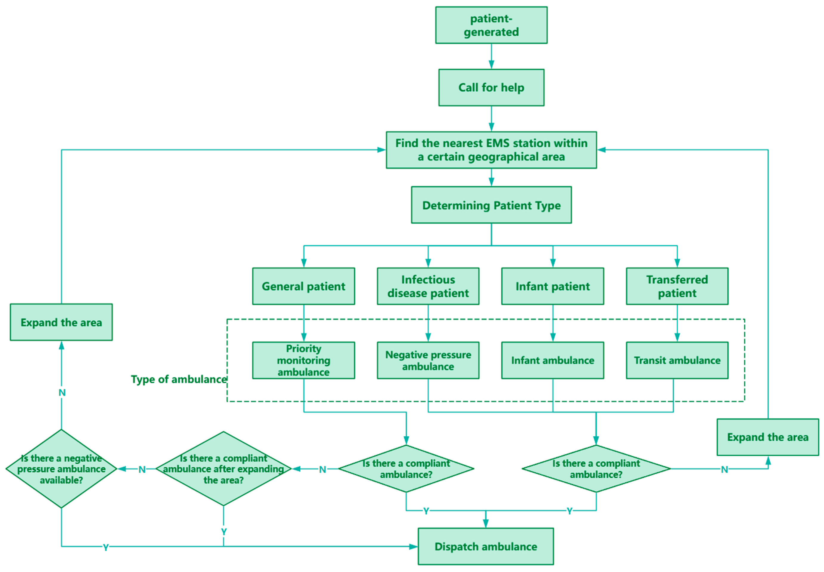
Once the patient generates and sends out a call for help, the model locates the nearest EMS station within a certain geographical area based on the specifics of the patient’s injuries. If a suitable EMS station cannot be located within the initial area, the search area is gradually expanded until an available EMS station is located. Once a station is identified, an ambulance is dispatched to the patient’s location.

Once the ambulance receives the patient, it will select the fastest route based on the current map and traffic condition information and quickly transport the patient to the nearest hospital for treatment. After completing the transportation task, the ambulance returns to the emergency network it belongs to for standby. There are four different types of ambulances in the model, and each type of ambulance provides services for different types or needs of patients. Figure 8 shows a flow chart of the patient evacuation process, which visually depicts the various aspects of the entire evacuation process.

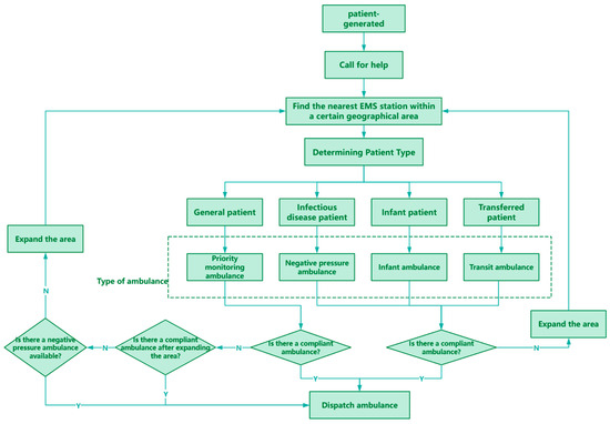
Figure 8. Patient evacuation process.

By analyzing the average time for ambulances to pick up patients obtained from different experiments, the performance of different strategies in Shanghai’s emergency evacuation system can be evaluated. Optimization recommendations are provided for the EMSS to improve the response time of the system, reduce the waiting time of patients, and increase the efficiency of treating patients. It also enables a better understanding and optimization of the Shanghai EMSS and provides effective decision support for Shanghai and even the national EMSS.

2.5.2. Constructing EMS Simulation Model

The main objects of the model include patients, hospitals, vehicle dispatchers, and ambulances, which are respectively modeled as agent objects [32]. In order to study the effect of the layout of the EMS stations on the average time taken to pick up patients, only ambulances were set up at the EMS stations, avoiding other interfering factors.

The model is divided into four stages, with three key stages being patient generation, call for help response, and patient evacuation, and the final stage being patient treatment and ambulance return. During the patient generation stage, the location and severity of the patient’s condition are determined based on historical data through random generation, ensuring the practical application value of the model. During the call for help response stage, the time from receiving a call for help at the emergency center to dispatching an ambulance was simulated. The patient evacuation stage can be divided into three processes: ambulance to the scene, on-site emergency treatment, and going to the hospital. During the process of waiting for an ambulance, if the waiting time exceeds the set threshold and the ambulance does not arrive, simulate the scenario of the patient going to the hospital on their own. The patient evacuation process simulates the process of an ambulance departing from the nearest EMS station to reach the patient’s location. After the ambulance arrives at the scene, emergency treatment should be given to the patient first, and then the patient should be transported to the nearest hospital for treatment. During this process, the driving path and time of the ambulance are influenced by geographic information such as road network and traffic conditions, ensuring that the simulation results are closer to the real situation.

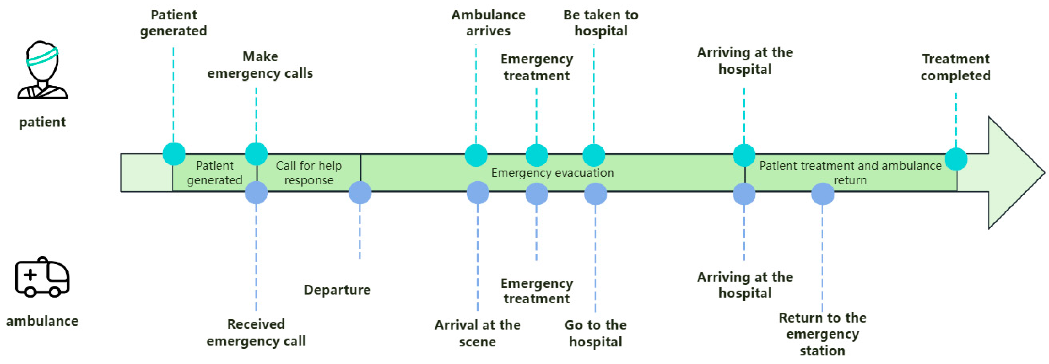
The simulation model is constructed according to Figure 9, in which the specific EMS evacuation process is built according to the description in 4.1, and the results of the analysis of the dataset are used as the parameters in the model to ensure that the model is real and reliable. In the simulation model, by inputting different EMS station layout schemes, the impact of different schemes on the average time for ambulances to pick up patients can be observed, and the effectiveness of optimizing the layout of EMS stations can be evaluated.

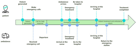
Figure 9. Overall timeline.

3. Experiment

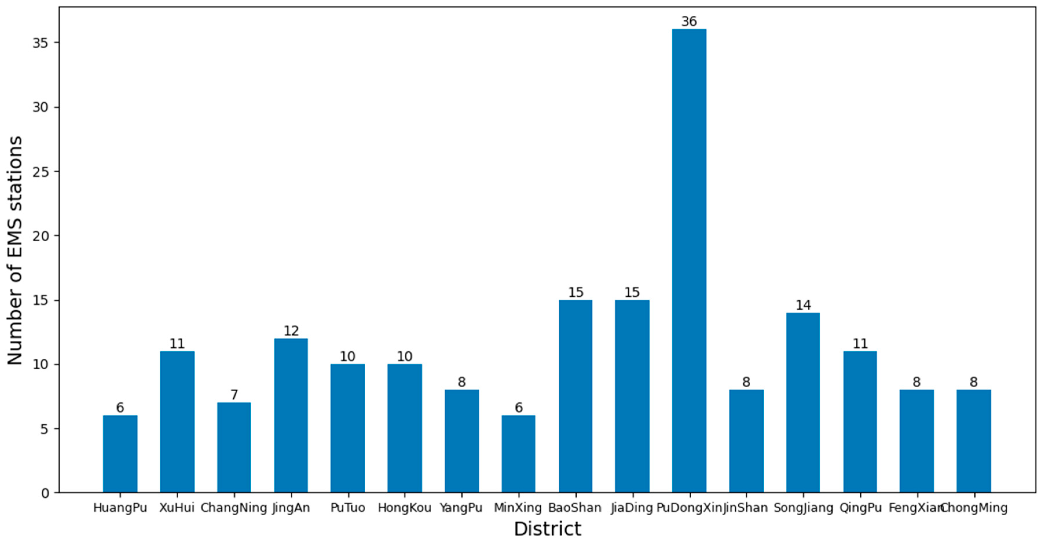
As of now, there are a total of 16 districts in Shanghai, and the number of EMS stations in each district is shown in Figure 10. To study the average time for ambulances to pick up patients when there are sufficient numbers of ambulances available.

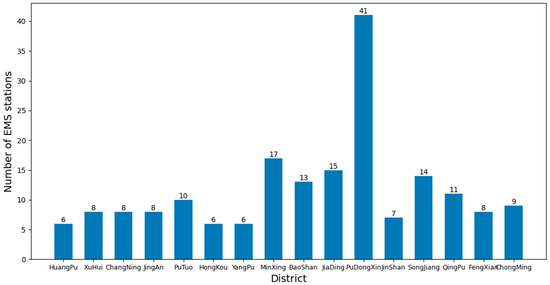
Figure 10. Number of EMS stations in each district of Shanghai.

By using the framework to analyze the dataset and control the k value in the k-means clustering algorithm, different layouts of EMS stations can be obtained. Then different layout information can be imported into the EMS simulation model to obtain the average time for an ambulance to pick up patients through different experiments. The average time obtained from the experiment is compared to evaluate the effectiveness of the algorithm and the authenticity and reliability of the model. Analysis and comparison can provide a deeper understanding of the impact of EMS station layout on rescue efficiency and provide guidance for future planning and optimization of EMSS. Figure 11 shows the experimental process.

Figure 11. Experimental process.

This paper conducted a total of four experiments, with the average time it takes for ambulances to pick up patients as the observation object, and eliminated the randomness caused by a certain experiment through Monte Carlo experiments. Experiment 1 involves importing data from existing EMS stations into a simulation model, while Experiment 2 maintains the same number of EMS stations in each district. Based on historical distress data, k-means clustering algorithm is used to determine the layout information of EMS stations in each district of Shanghai, and the obtained location information is imported into the simulation model. Experiment 3 uses the k-means clustering algorithm combined with the elbow method and silhouette coefficient method to determine the optimal number and layout information of EMS stations in each district of Shanghai, and also imports the obtained location information into the simulation model. By comparing the average time taken by ambulances to pick up patients in three different experimental scenarios, it is possible to quantitatively evaluate the specific impact of optimizing the layout of EMS stations on rescue efficiency and provide empirical support for further planning and improvement of EMSS. Experiment 4 is a robustness experiment conducted on the basis of Experiment 3, randomly selecting n EMS stations to make them unavailable, i.e., losing the ability to dispatch ambulances, in order to evaluate the stability and reliability of the model through evaluation indicators.

3.1. Efficiency Evaluation Experiment on the Layout of Existing EMS Stations

In order to simulate the real situation, first, import the data of the existing EMS stations in Shanghai into the simulation model and conduct Monte Carlo experiments. A Monte Carlo experiment [12] is a simulation method based on random sampling used to simulate the behavior and prediction results of complex systems. Its main purpose is to approximate the behavior of the system by generating a large number of random samples in order to evaluate and analyze the system. Monte Carlo experiments can help evaluate the stability and risk of a system when facing uncertain factors. The models were run for 500, 1000, and 1500 min, respectively, with 100 iterations. The average time consumption for each iteration is calculated as shown in the following formula.

$$\mathrm{T}={\sum }_{i=0}^n{t}_{i}P\left(i\right),$$

(3)

Here, $i$ represents the $i$-th time interval, n represents the total number of time intervals, and $t_i$ represents the average time of the i-th time interval, which is the average of the minimum and maximum time of the i-th time interval. $P\left(i\right)$ represents the probability that the average time of receiving patients falls within the i-th time interval after 100 experimental iterations. The average time required for an ambulance to pick up patients is shown in Table 6.

Table 6. Average time taken to pick up patients in Experiment 1.

	Model Run Time (Minutes)			Average
	500	1000	1500
Real value (minutes)	10.932			10.932
Experiment 1 result (minutes)	11.058	11.011	11.031	11.033

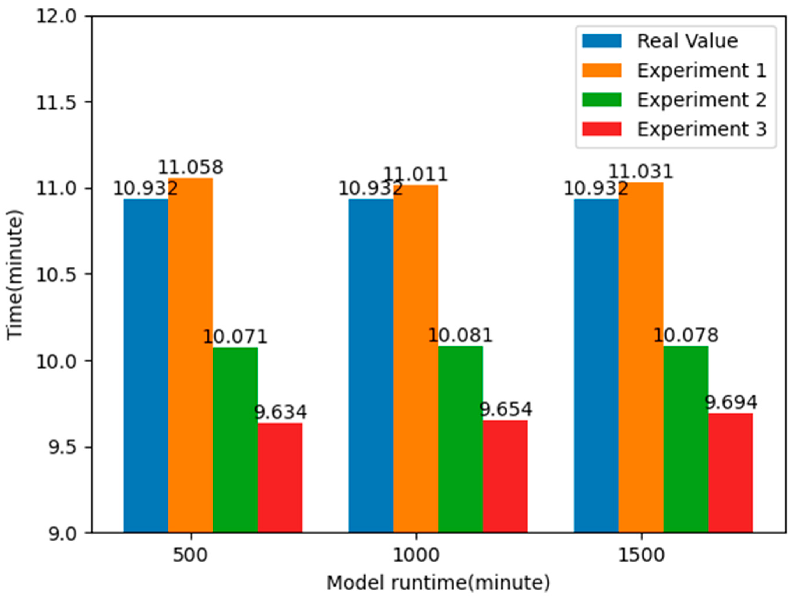
From the above table, it can be seen that without using the k-means clustering algorithm to optimize the layout of EMS stations, the average time for ambulances to pick up patients is about 11.033 min. By analyzing the data in the emergency patient call record dataset, it was found that the actual average time for an ambulance to pick up patients was 10.932 min, while the average time obtained in the simulation model was 11.033 min, with a difference of 0.101 min, less than a second. This also proves the authenticity and reliability of the simulation model.

3.2. Layout Optimization Experiment Driven by Historical Demand

Next, proceed to the second experiment. Keeping the number of EMS stations in each district constant, based on the historical call dataset, use k-means clustering algorithm to determine the layout information of EMS stations in each district and import the obtained location information into the simulation model. Perform Monte Carlo experiments again, running the models for 500, 1000, and 1500 min, respectively, with 100 iterations. In this way, the average time it takes for ambulances to pick up patients optimized by the k-means clustering algorithm can be obtained. The experimental results are shown in Table 7.

Table 7. Average time taken to pick up patients in Experiment 2.

		Model Run Time (Minutes)			Average
		500	1000	1500
Real value (minutes)		10.932			10.932
Experiment 1 result (minutes)		11.058	11.011	11.031	11.033
Experiment 2 result (minutes)		10.071	10.081	10.078	10.077
Percentage reduction in time for Experiment 2	Compared to the real value	7.876%	7.784%	7.812%	7.824%
	Compared to Experiment 1	8.926%	8.446%	8.639%	8.670%

By comparing the results of the two experiments, it can be found that by applying the k-means clustering algorithm to optimize the layout of the EMS stations, the average time taken to pick up patients is reduced by about 7.824%, nearly one minute, compared to the real value, and about 8.670%, about one minute or so, compared to Experiment 1. This shows that by optimizing the layout information of the EMS stations, it is possible to respond to emergencies faster, effectively improve the rate of patient rescue, and allocate emergency resources more effectively to the places where they are needed, thus reducing the time spent on receiving patients. The experimental results are shown in Figure 12.

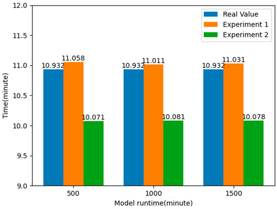
Figure 12. Comparison of average response time of patients after optimizing the location of EMS stations.

3.3. Experiments on the Optimal Configuration of the Number of EMS Stations and Layout

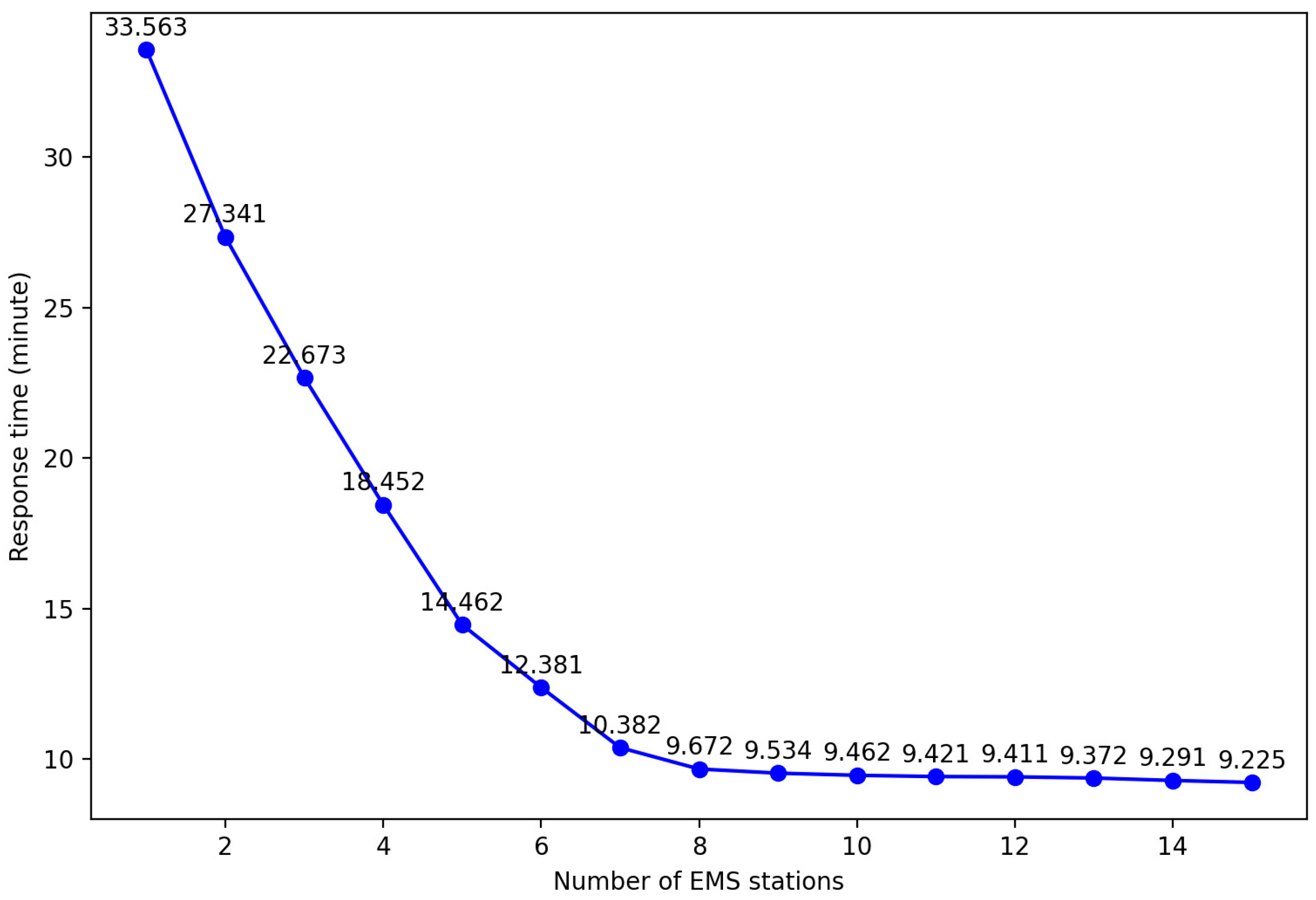
In order to obtain the optimal layout plan for EMS stations required in each region of Shanghai, it is first necessary to explore the impact of different EMS stations on the average response time, that is, the influence of different k values on the experimental results. Taking Yangpu District, Shanghai, as an example, by setting different k values and controlling the same number of ambulances, the impact on the average response time was observed. The results are shown in the table.

By analyzing Figure 13, it can be found that increasing the number of EMS stations can effectively shorten the average response time. However, when the number of stations reaches a certain threshold, the improvement in average response time tends to plateau. This is because with a fixed total number of ambulances, an increase in the number of stations may allow some patients to receive treatment faster, but it also leads to a decrease in the number of ambulances that can be deployed at each station. Once the ambulance at a certain station is insufficient to respond to emergency calls within the service area, it is necessary to allocate vehicles from other stations, which can actually prolong the average response time. Therefore, an excessive increase in EMS sites not only fails to further reduce the average response time but also brings unnecessary economic burdens due to the rise in site construction and operation costs. So, this paper uses an improved k-means clustering algorithm to obtain the optimal layout plan for each district.

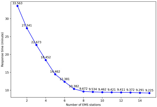
Figure 13. Average response time results of different EMS stations in Yangpu district.

First, the districts are clustered using the k-means clustering algorithm, which performs an elbow method analysis by trying different numbers of k clusters and calculating the sum-of-squares error within each cluster. By plotting the relationship between the number of clusters k and the SSE, we can observe the elbow of the curve, which is the point at which the decrease in variance due to an increase in the number of clusters gradually slows down. This elbow corresponds to the optimal number of k clusters.

In addition, the quality of the clusters can be assessed using the silhouette coefficient method. The silhouette coefficient combines the closeness within clusters and the separation between clusters, and its value ranges from −1 to 1. A higher silhouette coefficient indicates high sample compactness within clusters and good separation between clusters. The mean silhouette coefficient is calculated for the different numbers of k clusters, and the value of k with a maximum mean silhouette coefficient is selected as the optimum number of clusters. Combining the elbow method and the silhouette coefficient method, the optimal number of EMS stations in each district of Shanghai is obtained, as shown in Figure 14.

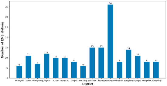
Figure 14. Optimized number of EMS stations in each district of Shanghai.

After determining the optimal number of k clusters, the correlation between response time and population density in different districts is a key factor in evaluating the effectiveness of station layout. Therefore, the number of ambulances at each station will be allocated based on the proportion of patient calls in each cluster. Input the obtained layout plan into the simulation model and conduct Monte Carlo experiments to simulate the process of ambulance picking up patients. The models were run for 500, 1000, and 1500 min, respectively, and iterated 100 times to obtain accurate results. By counting the average time taken by the ambulance to pick up the patient in these experiments, the effect of the different number of EMS stations can be evaluated. The average time taken to pick up patients is shown in Table 8.

Table 8. Average time taken to pick up patients in Experiment 3.

		Model Run Time (Minutes)			Average
		500	1000	1500
Real value (minutes)		10.932			10.932
Experiment 1 result (minutes)		11.058	11.011	11.031	11.033
Experiment 2 result (minutes)		10.071	10.081	10.078	10.077
Experiment 3 result (minutes)		9.634	9.654	9.694	9.661
Percentage reduction in time for Experiment 3	Compared to the real value	11.873%	11.690%	11.325%	11.629%
	Compared to Experiment 1	12.878%	12.324%	12.120%	12.441%
	Compared to Experiment 2	4.339%	4.236%	3.810%	4.128%

After the optimal configuration of the EMS stations, as shown in Figure 12, the number of EMS stations in some districts did not change, while in some districts it decreased and in others it increased. However, the average time taken to pick up patients decreased by more than 20 s, about 4.128%, based on Experiment 2; 1.271 min, about 11.629%, based on the actual value; and 1.372 min, about 12.441%, based on Experiment 1, greatly reducing the average time taken to pick up patients. Figure 15 shows the comparison of the average time taken to pick up patients. This will provide effective guidance for EMS in Shanghai, optimizing the layout and response time of EMS and thereby improving rescue efficiency and patient survival rate.

Figure 15. Comparison of average response time of patients under optimal EMS stations layout.

3.4. Performance Evaluation of EMS Simulation Model

In the process of optimizing the layout of EMS stations to improve rescue efficiency, what needs to be considered is not only the theoretical efficiency improvement but also to ensure that this layout can cope with various emergencies and changes in real situations, i.e., the robustness of the system. Robustness testing usually involves two aspects: sensitivity analysis and scenario simulation experiments [33].

For sensitivity analysis, this step involves adjusting the model input parameters and algorithm assumptions and observing how these changes affect the output results. For example, the number or location of emergency stations can be adjusted and the impact of these adjustments on the overall rescue response time can be assessed. As for scenario simulation experiments, random factors and data variations are introduced to simulate different emergencies in order to be closer to the actual situation. For example, it can be randomly set that a certain EMS station is unable to dispatch an ambulance normally due to malfunction or other reasons, so as to assess the response and handling capacity of other stations.

In the robustness experiment, if an EMS station is unavailable, the emergency requests that should have been responded to by that station need to be transferred to other stations. This may lead to an increase in waiting time, but by simulating such a scenario, the adaptability and stability of the whole system in the face of unexpected events can be evaluated.

Overall, rigorous testing of the robustness of the EMS station layout ensures that in real-world operations, even in the face of uncertainties, this system will still be able to respond effectively to emergencies and ensure that patient rescue times are minimized. By conducting robustness tests on the optimized layout of emergency stations, it has been proven that the optimized layout can effectively respond to unexpected situations in reality.

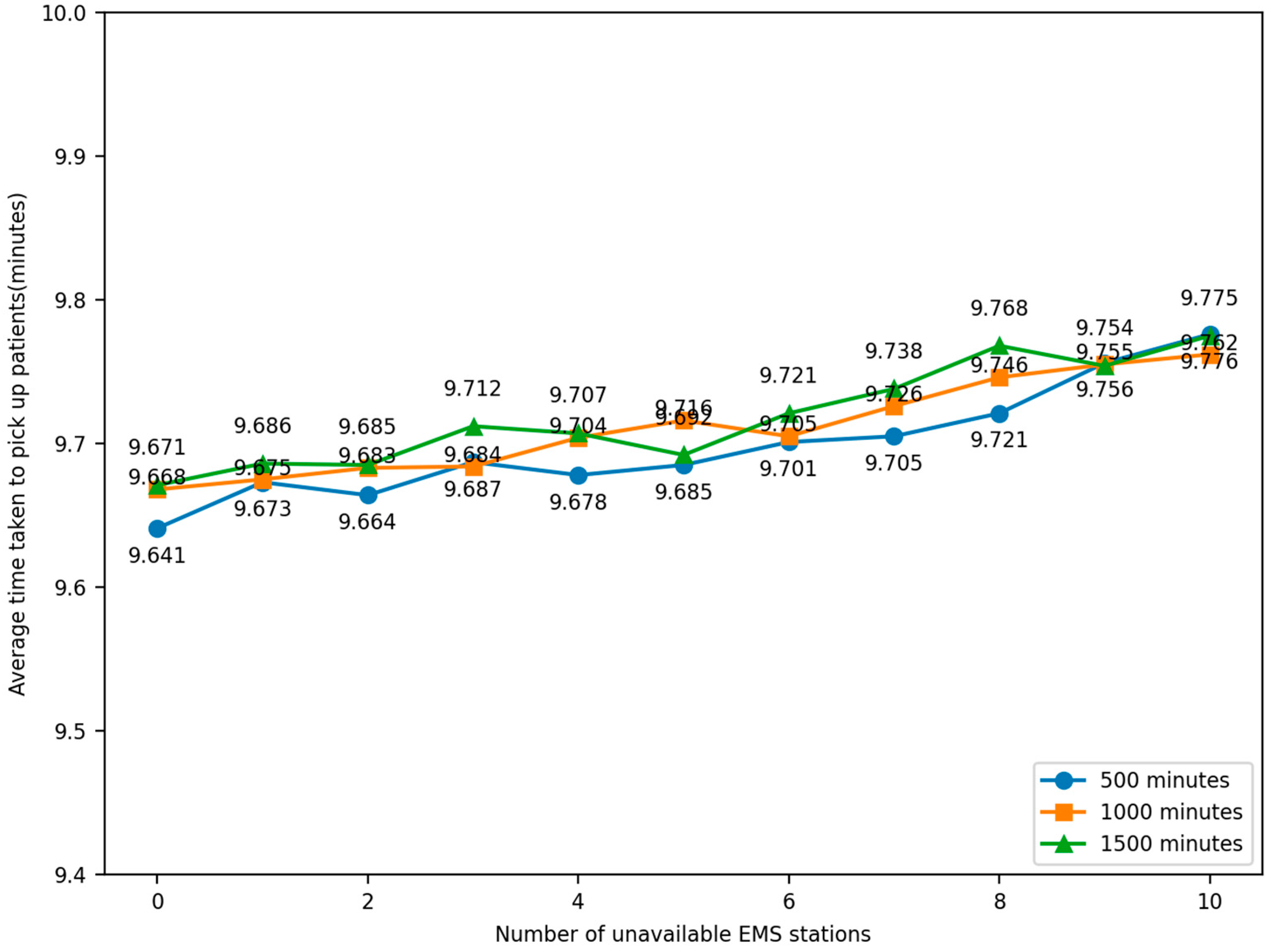
The experiment was conducted by randomly selecting the locations of EMS stations so that they lost the ability to dispatch ambulances. The number of unavailable EMS stations, 1–10, was compared to the average time taken by ambulances to pick up patients under normal conditions, and the change in time was observed. The simulation was iterated 100 times and the model was run for 500, 1000, and 1500 min. The relationship between the number of faulty EMS stations and the average elapsed time for an ambulance to pick up patients in the simulation model was obtained, as shown in Figure 16.

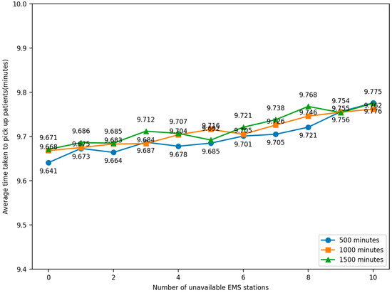
Figure 16. Robustness experiment result.

Through sensitivity analysis and a simulation of experiments in different scenarios, observing the data, it can be seen that the average time taken to pick up patients is no more than 9.8 min, which is shorter than the average time taken in both Experiment 1 and Experiment 2, proving that the optimized scheme can still provide a better rescue effect in different scenarios and can be considered to have a certain degree of robustness. This helps to better cope with uncertainties and changes in practical applications and provide more reliable and efficient EMS.

4. Conclusions and Future Work

In order to reduce the average time for ambulances to pick up patients, this paper proposes a decision support framework for optimizing the layout of EMS stations. The framework first analyzes the dataset of historical patient call records and then uses the k-means clustering algorithm to cluster and analyze the geographic location information of patient call records in the dataset. A simulation model for EMS is established to verify the effectiveness and reliability of the algorithm.

In the framework, the effectiveness of the simulation model was first verified by comparing real data and simulation data. Secondly, by controlling the number of EMS stations in each district of Shanghai (which is the same as the existing number of stations), the k-means algorithm was used to cluster and analyze historical data. The obtained EMS station information was then imported into the simulation model to observe the changes in the average time for ambulances to pick up patients. The experimental results show that after using the k-means clustering algorithm for analysis, the average time for ambulances to pick up patients can be reduced to 10.077 min, a decrease of 8.670%.

Afterwards, the k-means algorithm is used in combination with the silhouette coefficient method and elbow method to determine the number of emergency stations in each district, which is the optimal value of k. By calculating the silhouette coefficient and sum of squares errors for different numbers of clusters, the optimal number of EMS stations required for each district can be determined. Applying the obtained location information of the EMS center to the simulation model, it was found that the average time taken to pick up patients was reduced by about one minute and twenty seconds compared to Experiment 1, about 12.441%. Through the study of emergency evacuation in Shanghai, this research not only provides strong support for optimizing the response time of EMS and improving the survival rate of patients in Shanghai but also offers decision-making support for pre-hospital EMS in China. Moreover, this optimization decision-making model can also be utilized in the layout decision-making scenarios of other similar municipal service stations, which broadens the application scope of the model and enriches the research implications for relevant fields.

Due to the fact that the number of ambulances is also one of the factors affecting the response time of EMS, future work will further consider this factor to achieve better service quality. Moreover, implementing proposed changes to the existing emergency medical service site layout will surely face complex challenges. Site relocations, for example, will bring extra costs, including transportation, construction, and equipment replacement. Also, the impact on the urban layout is significant, potentially changing traffic flow and functional zoning. Thus, when making site changes, systematic analysis across economic, planning, and social aspects is essential to provide a solid basis for optimizing the layout scientifically.

References

- Colla, M.; Oliveira, G.; Santos, G. Operations Management in Emergency Medical Services: Response Time in a Brazilian Mobile Emergency Care Service. Procedia Manuf. 2019, 39, 932–941. [Google Scholar] [CrossRef]
- Hiestand, B.; Moseley, M.; MacWilliams, B.; Southwick, J. The influence of emergency medical services transport on Emergency Severity Index triage level for patients with abdominal pain. Acad. Emerg. Med. Off. J. Soc. Acad. Emerg. Med. 2011, 18, 261–266. [Google Scholar] [CrossRef] [PubMed]
- He, Z.; Qin, X.; Xie, Y.; Guo, J. Service Location Optimization Model for Improving Rural Emergency Medical Services. Transp. Res. Rec. 2018, 2672, 83–93. [Google Scholar] [CrossRef]
- Deng, Y.; Zhang, Y.; Pan, J. Optimization for locating emergency medical service facilities: A case study for health planning from China. Risk Manag. Healthc. Policy 2021, 14, 1791–1802. [Google Scholar] [CrossRef]
- Golabian, H.; Arkat, J.; Farughi, H.; Tavakkoli-Moghaddam, R. A simulation-optimization algorithm for return strategies in emergency medical systems. Simulation 2021, 97, 565–588. [Google Scholar] [CrossRef]
- Aboueljinane, L.; Sahin, E.; Jemai, Z. A discrete simulation-based optimization approach for multi-period redeployment in emergency medical services. Simulation 2023, 99, 659–679. [Google Scholar] [CrossRef]
- Alisan, O.; Ulak, M.B.; Ozguven, E.E.; Horner, M.W. Location selection of field hospitals amid COVID-19 considering effectiveness and fairness: A case study of Florida. Int. J. Disaster Risk Reduct. 2023, 93, 103794. [Google Scholar] [CrossRef]
- Akpınar, M.E.; Ilgın, M.A. Location selection for a Covid-19 field hospital using fuzzy choquet integral method. Gümüşhane Üniversitesi Sos. Bilim. Derg. 2021, 12, 1095–1109. [Google Scholar]
- Zhang, Z.; Hu, Y.; Lu, W.; Cao, W.; Gao, X. Spatial accessibility analysis and location optimization of emergency shelters in Deyang. Geomat. Nat. Hazards Risk 2023, 14, 1. [Google Scholar] [CrossRef]
- Hassan, S.A.; Alnowibet, K.; Agrawal, P.; Mohamed, A.W. Optimum Location of Field Hospitals for COVID-19: A Nonlinear Binary Metaheuristic Algorithm. Comput. Mater. Contin. 2021, 68, 1183–1202. [Google Scholar] [CrossRef]
- Grot, M. Decision support framework for tactical emergency medical service location planning. Omega 2024, 125, 103036. [Google Scholar] [CrossRef]
- Wang, X.; Shao, C.; Xu, S.; Zhang, S.; Xu, W.; Guan, Y. Study on the Location of Private Clinics Based on K-Means Clustering Method and an Integrated Evaluation Model. IEEE Access 2020, 8, 23069–23081. [Google Scholar] [CrossRef]
- Han, B.; Hu, M.; Wang, J. Site selection for pre-hospital emergency stations based on the actual spatiotemporal demand: A case study of Nanjing City, China. ISPRS Int. J. Geo-Inf. 2020, 9, 559. [Google Scholar] [CrossRef]
- Wang, Z. Base station planning problem based on genetic algorithm and K-Means clustering algorithm. In Proceedings of the 2023 IEEE 2nd International Conference on Electrical Engineering, Big Data and Algorithms (EEBDA), Changchun, China, 24–26 February 2023; IEEE: Piscataway, NJ, USA, 2023; pp. 747–752. [Google Scholar]
- Luo, R. A study of base station establishment site selection based on cluster analysis. In Proceedings of the 2023 IEEE 2nd International Conference on Electrical Engineering, Big Data and Algorithms (EEBDA), Changchun, China, 24–26 February 2023; IEEE: Piscataway, NJ, USA, 2023; pp. 686–691. [Google Scholar]
- Fan, B. Spatial clustering mining method for site selection problem of emergency response center. J. Manag. Sci. China 2008, 11, 16–24+26–28. [Google Scholar]
- Sonta, A.; Dougherty, T.R.; Jain, R.K. Data-driven optimization of building layouts for energy efficiency. Energy Build. 2021, 238, 110815. [Google Scholar] [CrossRef]
- Lin, T.; Liu, Y.; Liu, B.; Wang, Y.; Wu, S.; Zhe, W. Hierarchical clustering framework for facility location selection with practical constraints. IET Cyber-Phys. Syst. Theory Appl. 2021, 6, 238–253. [Google Scholar] [CrossRef]
- Yu, W.; Liu, X.; Chen, H.; Xue, C.; Zhang, L. Research of an emergency medical system for mass casualty incidents in Shanghai, China: A system dynamics model. Patient Prefer. Adherence 2018, 12, 207–222. [Google Scholar] [CrossRef]
- Wu, I.C.; Lin, Y.C.; Yien, H.W.; Shih, F.Y. Constructing constraint-based simulation system for creating emergency evacuation plans: A case of an outpatient chemotherapy area at a cancer medical center. Healthcare 2020, 8, 137. [Google Scholar] [CrossRef]
- Traoré, M.K.; Zacharewicz, G.; Duboz, R.; Zeigler, B. Modeling and simulation framework for value-based healthcare systems. Simulation 2019, 95, 481–497. [Google Scholar] [CrossRef]
- Nogueira, L.C.; Pinto, L.R.; Silva PM, S. Reducing Emergency Medical Service response time via the reallocation of ambulance bases. Health Care Manag. Sci. 2016, 19, 31–42. [Google Scholar] [CrossRef]
- Oliveira, B.R.; De Vasconcelos, J.A.; Almeida, J.F.; Pinto, L.R. A Simulation-Optimisation approach for hospital beds allocation. Int. J. Med. Inform. 2020, 141, 104174. [Google Scholar] [CrossRef] [PubMed]
- Khan, S.I.; Hoque AS, M.L. SICE: An improved missing data imputation technique. J. Big Data 2020, 7, 37. [Google Scholar] [CrossRef]
- Zhang, Z. Missing values in big data research: Some basic skills. Ann. Transl. Med. 2015, 3, 323. [Google Scholar]
- Anil, K.J. Data clustering: 50 years beyond K-Means. Pattern Recognit. Lett. 2010, 31, 651–666. [Google Scholar]
- Zubair, M.; Iqbal, M.A.; Shil, A.; Chowdhury, M.J.; Moni, M.A.; Sarker, I.H. An improved K-means clustering algorithm towards an efficient data-driven modeling. Ann. Data Sci. 2022, 11, 1525–1544. [Google Scholar] [CrossRef]
- Ahmed, M.; Seraj, R.; Islam SM, S. The k-means algorithm: A comprehensive survey and performance evaluation. Electronics 2020, 9, 1295. [Google Scholar] [CrossRef]
- Huiling, Z. Design and Implementation of an Improved K-Means Clustering Algorithm. Mob. Inf. Syst. 2022, 2022, 6041484. [Google Scholar]
- Liu, F.; Juan, Y.; Yao, L. Research on the number of clusters in K-means clustering algorithm. Electron. Des. Eng. 2017, 25, 9–13. [Google Scholar]
- Lei, T.; Li, S. Improved K-means clustering algorithm by combining with multiple factors. In Proceedings of the 2021 3rd International Conference on Advances in Computer Technology, Information Science and Communication (CTISC), Shanghai, China, 23–25 April 2021; IEEE: Piscataway, NJ, USA, 2021; pp. 258–263. [Google Scholar]
- Taghizadeh, M.; Mahsuli, M.; Poorzahedy, H. Probabilistic framework for evaluating the seismic resilience of transportation systems during emergency medical response. Reliab. Eng. Syst. Saf. 2023, 236, 109255. [Google Scholar] [CrossRef]
- Vander Heyden, Y.; Nijhuis, A.; Smeyers-Verbeke, J.; Vandeginste, B.G.; Massart, D.L. Guidance for robustness/ruggedness tests in method validation. J. Pharm. Biomed. Anal. 2001, 24, 723–753. [Google Scholar] [CrossRef] [PubMed]
Disclaimer/Publisher’s Note: The statements, opinions and data contained in all publications are solely those of the individual author(s) and contributor(s) and not of MDPI and/or the editor(s). MDPI and/or the editor(s) disclaim responsibility for any injury to people or property resulting from any ideas, methods, instructions or products referred to in the content. |
© 2025 by the authors. Licensee MDPI, Basel, Switzerland. This article is an open access article distributed under the terms and conditions of the Creative Commons Attribution (CC BY) license (https://creativecommons.org/licenses/by/4.0/).