The Impact of R&D Subsidy and IPP on Global Supply Chain Networks System—A Technology Spillover Perspective

Abstract

In the current globalized business environment, multinational competition has become the norm for companies. This paper considers technology spillovers among manufacturers and develops a global supply chain network equilibrium model. Firstly, the optimal decision-making behaviors of manufacturers, retailers, and demand markets are characterized separately. Secondly, based on the variational inequality theory, the optimal decision-making behaviors of global supply chain members are transformed. Finally, the model is solved and analyzed using the Euler algorithm. The primary objective is to explore the impact of research and development (R&D) subsidies and intellectual property protection (IPP) strategies on manufacturers’ research and development technological levels. Furthermore, the study delves into their effects on the production and transactions of the global supply chain network and social welfare. The following conclusions are drawn: (1) Technology spillovers have a positive effect on the technological level achieved by manufacturers through research and development investment and social welfare. However, intense technological competition may harm manufacturers’ profits. (2) Under the symmetric subsidy policy, higher subsidies may lead to a decrease in social welfare. (3) Under symmetric intellectual property protection policies, increasing the intensity of intellectual property protection benefits manufacturers but is detrimental to retailers and social welfare. However, under an asymmetric intellectual property protection strategy, implementing high-intensity intellectual property protection by high-technology countries is advantageous for retailers and social welfare. This conclusion has contributed to the technical research and development and production operation decision making of global supply chain members, as well as government policy formulation, and has also provided a new perspective for theoretical research in the field of global supply networks.

1. Introduction

With the ongoing deepening of globalization, the business relationships among multinational enterprises have grown increasingly intricate, characterized by intensified competition within the same level and coupling between upper and lower levels of the supply chain. As a result, the decisions of any individual enterprise not only affect itself but also impact other interconnected companies [1]. To maintain a competitive advantage in the dynamic global supply chain network, brimming with both challenges and opportunities, enterprises have been vigorously investing in R&D. For instance, in 2019, Alphabet allocated a substantial investment of up to EUR 18.3 billion to advance their technical R&D activities. Similarly, Huawei also invested EUR 12.7 billion in technical R&D, focusing on innovation and technological progress in the field of electronic products. Additionally, companies like Intel and Roche have devoted nearly 20% of their revenue to technological R&D [2].

Engaging in R&D not only helps improve competitiveness and market position for companies but also enhances innovation capabilities, providing a sturdy groundwork for sustainable development. A prime example of this is Huawei, which has achieved remarkable milestones through its relentless pursuit of innovation and R&D. As a result, the company has garnered widespread acclaim in the technology industry and the global business arena, while also making substantial contributions to the advancement and progress of China [3].

In recent times, governments around the world have been actively implementing subsidy policies to encourage companies to strengthen their technological R&D. For instance, in June 2021, the US Senate passed the Innovation and Competition Act, earmarking a substantial USD 250 billion for research subsidies to support innovative technological R&D activities conducted by businesses and research institutions [4]. Similarly, the Russian government has put forward the “Russian Technology Year”, which is expected to provide funding of over RUB 2.1 trillion to support technological R&D [5]. In a similar vein, the UK government has launched the “UK Research and Development Roadmap”, with the aim of investing GBP 22 billion in R&D funding by 2025. Furthermore, the UK government has made a commitment to increase R&D expenditure to 2.4% of GDP by 2027, with the overarching goal of promoting innovation and driving economic growth [6]. In 2018, the Chinese government allocated a budget of CNY 200 billion for research and development initiatives [2].

However, during the production and operation process within the global supply chain network, the technological R&D achievements of any enterprise inevitably spill over to other companies [7]. This phenomenon often enables these enterprises to rapidly gain access to technology and market share through means such as imitation, theft, or infringement, without the need for extensive research and genuine innovative efforts. For example, in 2021, a Fortune 500 company directly utilized Midea Group’s magnetic topology structure scheme in GMCC compressor technology¹. Prior to this, the LED industry has witnessed frequent cases of patent infringement lawsuits involving companies such as Seoul Semiconductor, Everlight Electronics, and Epistar². These instances of technology spillover not only harm the interests of the original innovators but also significantly affect the decisions of other members within the global supply chain network [8].

To prevent technology spillovers and safeguard the interests of innovators, governments worldwide have been strengthening IPP [9]. IPP grants technology developers exclusive rights to their intellectual achievements for a certain period, effectively reducing the risk of technology spillovers [10]. However, IPP policies can also have a dampening effect on innovation activities. For instance, in the 1980s, the United States government enacted the “Bayh-Dole” Act, allowing American universities to patent research outcomes funded by government grants. While this increased the number of patents held by US universities, it also restricted the societal spillover of knowledge from universities and constrained subsequent innovations within the industry [11].

The influence of R&D subsidies and IPP policies on technological innovation in companies is exceptionally complex, with significant differences in technological capabilities and R&D investments among manufacturers from different countries. Moreover, decisions made by any single member within the global supply chain network have ramifications on other members [1]. Therefore, within the framework of a global supply chain network system, contemplating the technology spillover effects and clarifying the mechanism of R&D subsidies and IPP policies on enterprise decision making is a deeply thought-provoking issue.

Based on this, the article considers the spillover effects of technological R&D in a competitive market and analyzes the behaviors and interactions of decision makers at various levels. By employing the variational inequalities theory and the Euler algorithm, this study derives equilibrium conditions for manufacturers, retailers, and the demand market to determine optimal behavior within the global supply chain network. The primary objective is to investigate the impact of government intervention policies, such as R&D subsidies and IPP, on the technological level of manufacturers, product transaction volume, profits, and social welfare. The paper addresses the following questions: Firstly, how does technological spillover affect output, the technological level of manufacturers, and the profits of enterprises in the global supply chain network? Secondly, what is the influence of government intervention strategies, such as R&D subsidies and IPP, on the technological level of manufacturers, profits, and social welfare within the global supply chain network? Finally, under symmetric and asymmetric intervention strategies, what decisions should be made by global supply chain network members? In contrast to the traditional perspective that focuses on technology spillover effects within one or two supply chains, adopting a global supply chain network perspective better reflects the dynamic nature of the real world. It captures the competitive and interconnected relationships among companies at the same level and across the upstream and downstream. This approach provides more comprehensive theoretical support for enterprise decision making and government policy formulation.

The remaining structure of the article is as follows: In Section 3, optimization models are developed individually for the manufacturer, retailer, and demand market layers. Subsequently, in Section 4, the qualitative properties of the solutions and the algorithms used to solve the models are discussed. Afterwards, to validate the effectiveness of the models, a series of numerical examples are designed in the fifth section. Finally, the relevant conclusions are presented in Section 6.

2. Literature Review

This article primarily focuses on three key areas of research: technology spillovers, government R&D subsidies and IPP, and supply chain network equilibrium.

2.1. Research on Technology Spillovers

Technology spillover refers to the diffusion of technology resulting from imitation among competing firms. Scholars have extensively analyzed and discussed technology spillover from various perspectives, including market structure, government intervention, green technology R&D, and carbon reduction. Among them, Levin and Reiss [12] studied the impact of imperfect product substitutability on technology R&D investment and found that, in certain cases, R&D investment costs increase due to technology spillover. Saaskilahti [13] investigated the relationship between network compatibility, technology spillover, and firms’ R&D investment. The study revealed that firms with lower technology levels reduce their R&D investment when the level of technology spillover decreases, and network compatibility negatively affects R&D investment. Jamali and Rasti-Barzoki [14] conducted research using the Stackelberg game model and found that government intervention policies and licensing contracts influence the optimal decision making of electric power companies. Yong et al. [15] explored the role of technology spillover in clean energy technology innovation and discovered that technology spillover inhibits firms from engaging in clean energy technology innovation. Yang and Nie [16] investigated the relationship between subsidies and clean innovation, suggesting that higher subsidy intensity leads to lower emissions and environmental efficiency. Orsatti [17] studied the relationship between government R&D budgets and green technology spillover based on relevant data, revealing that higher government R&D budgets promote technology spillover.

However, the existing literature predominantly focuses on examining the impact of technology spillover on firm decision making from a game theory perspective. Yet research on spillover effects is still limited, particularly in complex global supply chain network environments. When multiple participants are involved, traditional game theory methods may not accurately capture the competition and coupling relationships among variables and stakeholders in the global supply chain network. Therefore, there is a need to explore the influence of firm R&D technology level and spillover effects on global supply chain networks, as it holds significant practical significance. This exploration not only aids enterprises in gaining a better understanding of technology spillover within global supply chain networks but also provides guidance for governments in formulating effective policies. By comprehending the dynamics of spillover effects in global supply chain networks, both enterprises and governments can make informed decisions to enhance competitiveness, innovation, and overall performance.

2.2. Research on R&D Subsidies and IPP

The importance of government intervention policies in competitive markets cannot be underestimated. This study focuses on two crucial policies, namely, R&D subsidies and IPP, which aim to incentivize R&D activities while effectively managing technology spillovers. In academia, the impact of government intervention strategies has emerged as a prominent and widely discussed topic of research and analysis.

In terms of government R&D subsidies, scholars have conducted research and analysis from various perspectives, including subsidy types and recipients. Firstly, different subsidy approaches have been explored, with a focus on production subsidies and unit R&D subsidies. For instance, Chen et al. [18] investigated the impact of production subsidies and innovation effort subsidies on firm R&D performance within a tripartite game involving the government, suppliers, and manufacturers. Their findings revealed that both types of subsidies do not contribute to cost reduction. On the other hand, Li et al. [19] developed a collaborative emission reduction model for manufacturers and retailers, examining the influence of government subsidies on technological R&D as well as marketing investments, and discovered that government subsidies can modify the optimal strategies of manufacturers and retailers. Han et al. [20] examined the effects of varying subsidy levels on product pricing in the new energy vehicle industry. Their research demonstrated a positive correlation between subsidy levels and product pricing, with subsidies playing an incentivizing role during the early stages of technology R&D and promotion. Moreover, He et al. [21] investigated the impact of different subsidy approaches on optimal emission reduction R&D decisions for firms, revealing that emission reduction R&D subsidies outperform emission quantity subsidies. Furthermore, several scholars have investigated the optimal strategies of supply chains under different subsidy recipients. For instance, Sun et al. [22] explored the optimal subsidy strategies at different R&D stages in the new energy vehicle industry and found that consumer subsidies are more effective in maximizing social welfare compared to production subsidies. Wei et al. [23] examined the supply chain cooperative emission reduction technology R&D strategies under consumer-side subsidies. In contrast to the aforementioned studies, this paper primarily focuses on government R&D subsidy strategies that specifically target production-side R&D investments. It aims to investigate the effects of different subsidies on the equilibrium decisions within the global supply chain network.

Regarding intellectual property protection, most studies utilize empirical methods to analyze the relationship between IPP and enterprise R&D. These studies suggest that strengthening IPP not only enhances the independent innovation capability of enterprises but also increase their profits. For instance, Branstetter et al. [24] examined the impact of IPP reform on multinational enterprises and found that strengthening IPP encourages firms to increase their technology investments. Skowronski and Benton [25] studied the issue of IPP in the outsourcing process and concluded that the strength of IPP determines the supplier’s investment costs. Xu et al. [26] explored the relationship between the intensity of IPP and R&D subsidies on technological innovation in the renewable energy sector. They found that IPP significantly regulates the impact of R&D subsidies on the innovation performance of renewable energy enterprises. Based on relevant data from multiple high-tech industries from 2004 to 2006, Wan et al. [27] explored the relationship between IPP and innovation efficiency and believe that IPP can improve the efficiency of enterprise transformation. On the other hand, Smith [28] argued that IPP inhibits the dissemination of technological R&D achievements, negatively impacting countries that rely on the diffusion of advanced technology to improve their technological level and hindering technological progress in society. Bessen and Maskin [29] contended that IPP fails to incentivize firms to engage in technological R&D, and excessive protection may harm firms’ innovation and profitability. Overall, scholars have mainly analyzed the impact of IPP on supply chains from an empirical standpoint, with a few deriving relevant relationships through mathematical modeling. This study considers the competitive and interdependent relationships among firms and constructs an equilibrium model for global supply chain networks to analyze the role of IPP in stimulating firms’ R&D and promoting market innovation vitality. Overall, scholars have mainly analyzed the impact of IPP on supply chains from an empirical standpoint, with a few deriving relevant relationships through mathematical modeling. This study considers the competitive and interdependent relationships among firms and constructs an equilibrium model for global supply chain networks to analyze the role of IPP in stimulating firms’ R&D and promoting market innovation vitality.

2.3. Supply Chain Network Equilibrium

With the acceleration of globalization and intensifying market competition, the business relationships among enterprises have become increasingly complex. To capture the competitive dynamics among peers and the interdependent relationships between upstream and downstream firms, Nagurney et al. [30] pioneered the development of a supply chain network equilibrium model, which depicted the optimal behaviors of different decision makers and their mutual interactions. This work laid the foundation for the evolution and advancement of supply chain network models. Subsequently, Nagurney and Toyasaki [31] constructed an equilibrium model for a reverse supply chain network, analyzing the sources, collection, and disposal of electronic waste from a network equilibrium perspective. Hammond and Beullens [32] extended the study of oligopoly supply chains to the realm of closed-loop supply chains, providing valuable insights. Furthermore, Ma et al. [33], considering customer time sensitivity and time costs, developed a supply chain network equilibrium model to examine optimal decisions under different production and service time choices. Throughout this process, numerous scholars have also extended the research on supply chain network equilibrium, encompassing various aspects such as multiproduct (Diabat and Jebali [34]), multiperiod (Diabat and Jebali [34]; Behzadi and Seifabrghy [35]), dynamic (Jabbarzadeh et al. [36]), loss aversion (Zhou et al. [37]), risk aversion (Rahimi et al. [38]), and inventory capacity (Zheng et al. [39]; Darmawan et al. [40]), among others. However, research on the technology spillover effects in the context of global supply chain networks remains limited.

After reviewing the literature on technology spillover, government R&D subsidies, IPP, and supply chain network equilibrium, it is evident that existing research covers a wide range of aspects. However, there are still opportunities for further expansion to better reflect real-world situations. Firstly, while a substantial portion of the technology spillover-related literature has primarily explored its impact on firm decisions from a game theory perspective, research on spillover effects in complex supply chain network environments remains relatively limited. Especially when dealing with numerous participants in the supply chain, traditional game theory methods become inadequate, making the supply chain network equilibrium approach more suitable. Consequently, there is a need to investigate the influence of firms’ R&D technology levels and spillover effects on supply chain network equilibrium decisions, as it holds both practical and theoretical significance. Secondly, the existing literature has mainly examined firm R&D decisions concerning R&D subsidies or IPP in isolation, with little consideration of the interactive effects of these factors on supply chain network equilibrium decisions. However, in the context of global supply chain networks, these interactions may play a pivotal role. Thus, this study endeavors to explore the impact of the interaction between R&D subsidies and IPP on global supply chain network equilibrium decisions. Furthermore, the study also considers the effects of asymmetric R&D subsidies and IPP on firm profits and social welfare, contributing significantly to the theory and practice of technology spillover in the context of global supply chain networks.

3. Model Construction

3.1. Problem Description

The global supply chain network involved in this study consists of T countries, each with I manufacturers, J retailers, and K demand markets. The products produced by different manufacturers exhibit partial substitutability. Within country $C_t$, retailer $R_{j_t}$ orders products from manufacturer $M_{i_t}$ and sells them in demand markets $S_{k_t}$, as shown in Figure 1. Here, $i\in \left\{1,\dots ,I\right\}, j\in \left\{1,\dots ,J\right\}, k\in \left\{1,\dots ,K\right\}, \mathrm{and} t\in \left\{1,\dots ,T\right\}$. Manufacturers or retailers within the same layer compete with each other, while upstream and downstream enterprises cooperate. In order to meet consumer demands and reduce production costs, $M_{i_t}$ invests in technological R&D and also benefits from the technology spillover effects introduced by other manufacturers.

Firstly, under the influence of R&D subsidies and IPP, manufacturers make decisions about the endogenous variables, including their technological level, production quantity, and transaction volume with retailers. Additionally, manufacturers also need to determine their exogenous prices, which include the wholesale prices of their products. Secondly, retailers are responsible for making decisions concerning their transactions with manufacturers and their transactions with the demand market, both of which are endogenous variables. Similarly, retailers need to determine their exogenous prices, including the retail price. Finally, the demand market determines the price that it is willing to pay for the product. The various symbols used in this study and their corresponding explanations are presented in

Table 1. Symbol description.

Symbols		Explanations
Parameters	$I$	Collection of manufacturers, $i\in \left\{1,\dots ,I\right\}$
	$J$	Collection of retailers,$j\in \left\{1,\dots ,J\right\}$
	$K$	Collection of demand markets $k\in \left\{1,\dots ,K\right\}$
	$T$	Collection of countries $t\in \left\{1,\dots ,T\right\}$
	$M_{i_t}$	Manufacturer i located in country t
	$R_{j_t}$	Retailer j located in country t
	$S_{k_t}$	Demand markets k located in country t
	$\mu$	The technology spillover rate between manufacturers $0\le \mu \le 1$, which can be determined based on relevant data disclosed by companies
	$b_{M_{i_t}}$	Subsidies provided by the country where the manufacturer is located for their R&D investment
	${\phi }_{M_{i_t}}$	The IPP intensity of manufacturer $M_{i_t}$, $0\le {\phi }_{M_{i_t}}\le 1$, which can be established in accordance with intellectual property policies enacted by individual countries
Decision variables	$q_{M_{i_t}}^{R_{j_t}}$	Transaction volume between $M_{i_t}$ and $R_{j_t}$
	$q_{M_{i_t}}$	Total transaction volume of $M_{i_t}$
	$p_{M_{i_t}}^{R_{j_t}}$	Wholesale price at which $M_{i_t}$ sells products to $R_{j_t}$
	$q_{M_{i_t}}^{R_{j_t}{S}_{k_t}}$	$R_{j_t}$ and $S_{k_t}$ on the transaction volume of $M_{i_t}$’s products
	$q_{M_{i_t}}^{S_{k_t}}$	The total demand for $M_{i_t}$’s products in the demand market $S_{k_t}$
	$p_{M_{i_t}}^{R_{j_t}{S}_{k_t}}$	The retail price of the product ordered by $R_{j_t}$ from $M_{i_t}$ in $S_{k_t}$
	$p_{M_{i_t}}^{S_{k_t}}$	The price that $S_{k_t}$ is willing to pay for the product of $M_{i_t}$
Functions	$d_{M_{i_t}}^{S_{k_t}}\left(p_{M_{i_t}}^{S_{k_t}},L_{M_{i_t}}\right)$	The demand function of $M_{i_t}$’s products in $S_{k_t}$
	$C_{M_{i_t}}\left(q_{M_{i_t}},L_{M_{i_t}}\right)$	The production cost function of $M_{i_t}$, which is influenced by the production and total technological level
	$C_{M_{i_t}}^{R\&D}\left({\omega }_{M_{i_t}}\right)$	The R&D cost function for $M_{i_t}$ when the R&D technology level is ${\omega }_{M_{i_t}}$
	$C_{M_{i_t}}^{\mathsf{\Omega }}\left(q_{M_{i_t}}^{R_{j_t}}\right)$	The transaction cost function between $M_{i_t}$ and $R_{j_t}$, borne by $M_{i_t}$
	$C_{R_{j_t}}^H\left(q_{M_{i_t}}^{R_{j_t}}\right)$	The handle cost function of $R_{j_t}$ for products from $M$, borne by $R_{j_t}$
	$C_{R_{j_t}}^{\Omega }\left(q_{M_{i_t}}^{R_{j_t}{S}_{k_t}}\right)$	The transaction cost function between $R_{j_t}$ and $S_{k_t}$ regarding $M_{i_t}$’s products, borne by $R_{j_t}$

.

To better characterize the research problem, based on the relevant literature, this paper proposes the following assumptions:

Assumption 1: 

In a global supply chain network, multiple manufacturers participate in the production of the same product and sell their products to different retailers to meet the needs of consumers in different demand markets [30]. Meanwhile, participants within the global supply chain network engage in a game with access to perfect information.

Assumption 2: 

Enterprises within the global supply chain network pursue the objective of profit maximization, and the functions involved in this study are all quadratic continuous and twice-differentiable convex functions.

Assumption 3: 

In an equilibrium state, both manufacturers and retailers achieve maximum profits, and they have no motivation to change their decisions. At this point, the total transaction volume between manufacturer $M_{i_t}$ and all retailers is equal to the production quantity of manufacturer $M_{i_t}$. Similarly, the total transaction volume between retailers and the demand market is equal to the purchasing quantity of retailers from all manufacturers [41,42].

3.2. Decisions at the Manufacturer Level

In a competitive market, manufacturers benefit from technological spillover effects by studying their competitors’ products. Let us assume that the technological spillover effect received by $M_{i_t}$ from its competitors is given by $\left(1-{\phi }_{M_{i_t}}\right)\frac{\mu {\omega }_{-M_{i_t}}}{IT-1}$, where ${\omega }_{-M_{i_t}}$ represents the sum of technological levels of all manufacturers except $M_{i_t}$ and IT$-$1 represents the total number of manufacturers excluding $M_{i_t}$. Thus, the technological level of $M_{i_t}$ can be expressed as $L_{M_{i_t}}={\omega }_{M_{i_t}}+\left(1-{\phi }_{M_{i_t}}\right)\frac{\mu {\omega }_{-M_{i_t}}}{IT-1}$ [43]. In the case of government subsidies for R&D investment, the actual cost for $M_{i_t}$ to invest in technological level ${\omega }_{M_{i_t}}$ is given by $\left(1-b_{M_{i_t}}\right)C_{M_{i_t}}^{R\&D}\left({\omega }_{M_{i_t}}\right)$. Additionally, $M_{i_t}$ incurs transaction costs when trading with $R_{j_t}$, denoted by $C_{M_{i_t}}^{\Omega }\left(q_{M_{i_t}}^{R_{j_t}}\right)$. In summary, the profit function of $M_{i_t}$ can be expressed as four parts, namely, sales revenue, production costs, R&D investment costs, and transaction costs. Then, the $M_{i_t}$’s optimization problem is given by (1):

$$\begin{array}{c}Max {\pi }_{M_{i_t}}={\displaystyle {\displaystyle \sum }_{t=1}^T}{\displaystyle {\displaystyle \sum }_{j=1}^J}{p}_{M_{i_t}}^{R_{j_t}}{q}_{M_{i_t}}^{R_{j_t}}-C_{M_{i_t}}\left(q_{M_{i_t}},L_{M_{i_t}}\right)\\ -\left(1-b_{M_{i_t}}\right)C_{M_{i_t}}^{R\&D}\left({\omega }_{M_{i_t}}\right)-C_{M_{i_t}}^{\Omega }\left(q_{M_{i_t}}^{R_{j_t}}\right)\\ \mathrm{s}.\mathrm{t}. q_{M_{i_t}}^{R_{j_t}}\ge 0, {\omega }_{M_{i_t}}\ge 0\end{array}$$

(1)

In the objective function, the cost functions involved are all convex and continuously differentiable. $M_{i_t}$ determines the transaction quantity ${q_{M_{i_t}}^{R_{j_t}}}^{*}$ and the R&D investment level ${{\omega }_{M_{i_t}}}^{*}$. Therefore, the optimal decision of $M_{i_t}$ satisfies the following variational inequality: ${\displaystyle {{\displaystyle \sum }}_{t=1}^T}{\displaystyle {{\displaystyle \sum }}_{i=1}^I}\left(\frac{\partial C_{M_{i_t}}^{\Omega }\left(q_{M_{i_t}}^{R_{j_t}}\right)}{\partial q_{M_{i_t}}^{R_{j_t}}}+\frac{\partial C_{M_{i_t}}(q_{M_{i_t}},L_{M_{i_t}})}{\partial q_{M_{i_t}}^{R_{j_t}}}-{p_{M_{i_t}}^{R_{j_t}}}^{*}\right)\left(q_{M_{i_t}}^{R_{j_t}}-{q_{M_{i_t}}^{R_{j_t}}}^{*}\right)+{\displaystyle {{\displaystyle \sum }}_{t=1}^T}{\displaystyle {{\displaystyle \sum }}_{i=1}^I}\left(\frac{\partial C_{M_{i_t}}\left(q_{M_{i_t}},L_{M_{i_t}}\right)}{\partial {\omega }_{M_{i_t}}}+\left(1-b_{M_{i_t}}\right)\frac{\partial C_{M_{i_t}}^{R\&D}\left({\omega }_{M_{i_t}}\right)}{\partial {\omega }_{M_{i_t}}}\right)\left({\omega }_{M_{i_t}}-{{\omega }_{M_{i_t}}}^{*}\right)\ge 0$, whereas $\forall ({q_{M_{i_t}}^{R_{j_t}}}^{*}$,${{\omega }_{M_{i_t}}}^{*})\in R_{+}^{IT\times JT}$.

The above equilibrium conditions have an economic explanation. When the wholesale price equals the sum of the marginal production costs and transaction costs associated with the manufacturer and the retailer, there is a positive transaction volume between the manufacturer and the retailer. However, if the sum of the manufacturer’s marginal production cost and transaction cost exceeds the wholesale price that the retailer is willing to pay for the product, the transaction volume between the manufacturer and the retailer becomes zero.

3.3. Decisions at the Retailer Level

$R_{j_t}$ purchases products from manufacturers and sells them in the demand market. Throughout this process, in addition to paying for the purchase cost of the products, $R_{j_t}$ also incurs handling costs, such as display and storage costs associated with the products. Hence, the profit function of $R_{j_t}$ can be expressed as four parts, namely, sales revenue, handling cost, transaction costs, and procurement cost. Then, the optimization problem of $R_{j_t}$ can be obtained by (2):

$$\begin{array}{c}\mathrm{Max}{\widehat{\pi }}_{R_{j_t}}={\displaystyle {\displaystyle \sum }_{t=1}^T}{\displaystyle {\displaystyle \sum }_{i=1}^I}{\displaystyle {\displaystyle \sum }_{k=1}^K}{p}_{M_{i_t}}^{R_{j_t}{S}_{k_t}}{q}_{M_{i_t}}^{R_{j_t}{S}_{k_t}}-C_{R_{j_t}}^H\left(q_{M_{i_t}}^{R_{j_t}}\right)\\ -C_{R_{j_t}}^{\Omega }\left(q_{M_{i_t}}^{R_{j_t}{S}_{k_t}}\right)-{\displaystyle {{\displaystyle \sum }}_{t=1}^T}{\displaystyle {{\displaystyle \sum }}_{i=1}^I}{p}_{M_{i_t}}^{R_{j_t}}{q}_{M_{i_t}}^{R_{j_t}}\\ \mathrm{s}.\mathrm{t}. q_{M_{i_t}}^{R_{j_t}{S}_{k_t}}\ge 0, q_{M_{i_t}}^{R_{j_t}}\ge 0\\ {\displaystyle {\displaystyle \sum }_{t=1}^T}{\displaystyle {\displaystyle \sum }_{k=1}^K}{q}_{M_{i_t}}^{R_{j_t}{S}_{k_t}}=q_{M_{i_t}}^{R_{j_t}}\end{array}$$

(2)

The constraint indicates that the total sales volume of $R_{j_t}$ to $S_{k_t}$ is equal to the total quantity purchased by $R_{j_t}$ from all manufacturers. In the case of non-cooperative competition, $R_{j_t}$ maximizes its profit by determining the optimal transaction quantity with the demand market, denoted as ${q_{M_{i_t}}^{R_{j_t}{S}_{k_t}}}^{*}$, and the expected quantity of goods obtained from manufacturers, denoted as ${q_{M_{i_t}}^{R_{j_t}}}^{*}$. The optimal decision of the retailer satisfies the following variational inequalities:

$$\begin{array}{c}{\displaystyle {\displaystyle \sum }_{t=1}^T}{\displaystyle {\displaystyle \sum }_{j=1}^J}\left(\frac{\partial C_{R_{j_t}}^H\left(q_{M_{i_t}}^{R_{j_t}}\right)}{\partial q_{M_{i_t}}^{R_{j_t}}}+{p_{M_{i_t}}^{R_{j_t}}}^{*}\right)\left(q_{M_{i_t}}^{R_{j_t}}-{q_{M_{i_t}}^{R_{j_t}}}^{*}\right)\\ +{\displaystyle {{\displaystyle \sum }}_{t=1}^T}{\displaystyle {{\displaystyle \sum }}_{j=1}^J}\left(\frac{\partial C_{R_{j_t}}^T\left(q_{M_{i_t}}^{R_{j_t}{S}_{k_t}}\right)}{\partial q_{M_{i_t}}^{R_{j_t}{S}_{k_t}}}-{p_{M_{i_t}}^{R_{j_t}{S}_{k_t}}}^{*}\right)\left(q_{M_{i_t}}^{R_{j_t}{S}_{k_t}}-{q_{M_{i_t}}^{R_{j_t}{S}_{k_t}}}^{*}\right)\ge 0\\ \forall \left({q_{M_{i_t}}^{R_{j_t}}}^{*}, {q_{M_{i_t}}^{R_{j_t}{S}_{k_t}}}^{*}\right)\in R_{+}^{IT\times JT\times KT}.\end{array}$$

(3)

3.4. Decisions at the Demand Market Level

The economic equilibrium conditions in the demand market can be expressed as follows: For any $R_{j_t}$, when the price accepted by consumers in the demand market equals the price set by the retailer, positive transactions occur in the market. Conversely, when the price accepted by consumers is lower than the price set by the retailer, market transactions become zero.

$${p_{M_{i_t}}^{S_{k_t}}}^{*}\{\begin{array}{c}={p_{M_{i_t}}^{R_{j_t}{S}_{k_t}}}^{*}, if {q_{M_{i_t}}^{R_{j_t}{S}_{k_t}}}^{*}>0\\ \ge {p_{M_{i_t}}^{R_{j_t}{S}_{k_t}}}^{*}, if {q_{M_{i_t}}^{R_{j_t}{S}_{k_t}}}^{*}=0\end{array}$$

(4)

When the quantity demanded in $S_{k_t}$ equals the total quantity of products purchased by consumers from $R_{j_t}$, the equilibrium price in the demand market is greater than zero. However, if the quantity demanded is less than the total quantity of products purchased by consumers from $R_{j_t}$, then the equilibrium price in the demand market is zero.

$${d_{M_{i_t}}^{S_{k_t}}}^{*}\{\begin{array}{c}={\displaystyle {{\displaystyle \sum }}_{t=1}^T}{\displaystyle {{\displaystyle \sum }}_{j=1}^J}{q_{M_{i_t}}^{R_{j_t}{S}_{k_t}}}^{*}, if {p_{M_{i_t}}^{S_{k_t}}}^{*}>0\\ \le {\displaystyle {{\displaystyle \sum }}_{t=1}^T}{\displaystyle {{\displaystyle \sum }}_{j=1}^J}{q_{M_{i_t}}^{R_{j_t}{S}_{k_t}}}^{*}, if {p_{M_{i_t}}^{S_{k_t}}}^{*}=0\end{array}$$

(5)

The equilibrium conditions of the demand market layer can be obtained as follows:

$$\begin{array}{c}{\displaystyle {{\displaystyle \sum }}_{t=1}^T}{\displaystyle {{\displaystyle \sum }}_{k=1}^K}({p_{M_{i_t}}^{R_{j_t}{S}_{k_t}}}^{*}-{p_{M_{i_t}}^{S_{k_t}}}^{*})\left(q_{M_{i_t}}^{R_{j_t}{S}_{k_t}}-{q_{M_{i_t}}^{R_{j_t}{S}_{k_t}}}^{*}\right)\\ +{\displaystyle {{\displaystyle \sum }}_{t=1}^T}{\displaystyle {{\displaystyle \sum }}_{k=1}^K}\left({\displaystyle {{\displaystyle \sum }}_{t=1}^T}{\displaystyle {{\displaystyle \sum }}_{j=1}^J}{q_{M_{i_t}}^{R_{j_t}{S}_{k_t}}}^{*}-{d_{M_{i_t}}^{S_{k_t}}}^{*}\right)\left(p_{M_{i_t}}^{S_{k_t}}-{p_{M_{i_t}}^{S_{k_t}}}^{*}\right)\ge 0 \\ \forall {p_{M_{i_t}}^{S_{k_t}}}^{*},{q_{M_{i_t}}^{R_{j_t}{S}_{k_t}}}^{*}\in R_{+}^{IT\times JT\times KT}\end{array}$$

(6)

3.5. Equilibrium Conditions of Global Supply Chain Networks

The optimal decisions within the global supply chain network must satisfy the equilibrium conditions of all manufacturers, retailers, and demand markets. As the variational inequalities exhibit additivity, the equilibrium conditions for the entire global supply chain network can be expressed as follows:

$$\begin{array}{c}{\displaystyle {\displaystyle \sum }_{t=1}^T}{\displaystyle {\displaystyle \sum }_{i=1}^I}\left[\frac{\partial C_{M_{i_t}}\left(q_{M_{i_t}},L_{M_{i_t}}\right)}{\partial q_{M_{i_t}}^{R_{j_t}}}+\frac{\partial C_{M_{j_t}}^{\mathsf{\Omega }}\left(q_{M_{i_t}}^{R_{j_t}}\right)}{\partial q_{M_{i_t}}^{R_{j_t}}}+\frac{\partial C_{R_{j_t}}^H\left(q_{M_{i_t}}^{R_{j_t}}\right)}{\partial q_{M_{i_t}}^{R_{j_t}}}\right]\left(q_{M_{i_t}}^{R_{j_t}}-{q_{M_{i_t}}^{R_{j_t}}}^{*}\right)\\ +{\displaystyle {\displaystyle \sum }_{t=1}^T}{\displaystyle {\displaystyle \sum }_{i=1}^I}\left[\frac{\partial C_{M_{i_t}}\left(q_{M_{i_t}},L_{M_{i_t}}\right)}{\partial {\omega }_{M_{i_t}}}+\left(1-b_{i_t}\right)\frac{\partial C_{M_{i_t}}^{R\&D}\left({\omega }_{M_{i_t}}\right)}{\partial {\omega }_{M_{i_t}}}\right]\left({\omega }_{M_{i_t}}-{{\omega }_{M_{M_{i_t}}}}^{*}\right)\\ +{\displaystyle {\displaystyle \sum }_{t=1}^T}{\displaystyle {\displaystyle \sum }_{j=1}^J}\left[\frac{\partial C_{R_{j_t}}^{\Omega }\left(q_{M_{i_t}}^{R_{j_t}{S}_{k_t}}\right)}{\partial q_{M_{i_t}}^{R_{j_t}{S}_{k_t}}}-p_{M_{i_t}}^{S_{k_t}*}\right]\left(q_{M_{i_t}}^{R_{j_t}{S}_{k_t}}-{q_{M_{i_t}}^{R_{j_t}{S}_{k_t}}}^{*}\right)\\ +{\displaystyle {{\displaystyle \sum }}_{t=1}^T}{\displaystyle {{\displaystyle \sum }}_{k=1}^K}\left({\displaystyle {{\displaystyle \sum }}_{t=1}^T}{\displaystyle {{\displaystyle \sum }}_{j=1}^J}{q_{M_{i_t}}^{R_{j_t}{S}_{k_t}}}^{*}-{d_{M_{i_t}}^{S_{k_t}}}^{*}\right)\left(p_{M_{i_t}}^{S_{k_t}}-{p_{M_{i_t}}^{S_{k_t}}}^{*}\right)\ge 0\end{array}$$

(7)

where $\forall \left({q_{M_{i_t}}^{R_{j_t}}}^{*},{{\omega }_{M_{i_t}}}^{*},{q_{M_{i_t}}^{R_{j_t}{S}_{k_t}}}^{*}, {p_{M_{i_t}}^{S_{k_t}}}^{*}\right)\in R_{+}^{IT\times JT\times KT}$.

4. Qualitative Properties of Solutions and Solving Algorithm

4.1. Qualitative Properties of Solutions

Variational inequalities were initially introduced by Lone and Tampacchia [44] and have since been extensively utilized to solve optimization problems. Over time, scholars like Nagurney have made continuous enhancements and advancements to this theory, making it widely applicable for solving finite-dimensional problems and addressing equilibrium problems in the field of economics. In recent years, both domestic and international scholars have recognized variational inequalities as a crucial tool for studying supply chain network equilibrium problems.

(1) Definitions of variational inequalities

Definition 1 

[45]. Let K be a non-empty subset in the n-dimensional Euclidean space $R^n$, and this subset is a given closed convex set.  $F\left(X\right)$is a continuous function defined on K and satisfies  $X^{*}\in K$. The variational inequality problem can be represented as  $VI\left(K, F\right)$, which involves finding a vector set  $X^{*}\in K$  such that for all  $X^{*}\in K$, the following condition holds:

$$F\left(X^{*}\right)·\left(X-X^{*}\right)\ge 0, \forall X\in K$$

(8)

Moreover, it can be expressed as an inner product in the following form:

Where 〈,〉 represents the inner product in the n-dimensional Euclidean space. The vector set $X^{*}$represents the solution set of the variational inequality problem.

(2) Existence and uniqueness of solutions

The existence and uniqueness of solutions depend on the properties of the non-empty subset K and the function $F\left(X\right)$.

Theorem 1 

([45]). When the non-empty subset K satisfies the following conditions: ① K is a bounded non-empty closed convex set, and the function $F\left(X\right)$ satisfies the following condition: ②  $F\left(X\right)$ is monotone and continuous on the bounded non-empty closed convex set K, then the variational inequality problem has at least one optimal solution.

Theorem 2 

([45]). When the non-empty subset K satisfies the following conditions: ① K is a bounded non-empty closed convex set, and the function $F\left(X\right)$ satisfies the following condition: ②  $F\left(X\right)$ is strictly monotone and continuous on set K, if the solution set of the variational inequality is non-empty, then the variational inequality has a unique solution.

The definition of strict monotony can be expressed as:

Definition 2 

([46]). If the following condition is satisfied:

$$❬F{\left(X^1-X^2\right)}^T,X^1-X^2❭\ge 0, \forall X^1,X^2\in K$$

(9)

then the function  $F\left(X\right)$  is said to be strictly monotone on the non-empty subset K.

In addition to the aforementioned theorems regarding the existence and uniqueness of solutions, the solution of the variational inequality can be described as a Nash equilibrium problem.

Definition 3 

([47]). The solution of a Nash equilibrium decision is a set of strategies, where there exists $X^{*}\in K$ such that:

$$U_m\left({X_m}^{*},{X_{-m}}^{*}\right)\ge U_m\left(X_m,{X_{-m}}^{*}\right), \forall m\in N, \forall X_m\in K$$

(10)

In the case that function $U_m$ is continuously differentiable and concave, the solution set $X^{*}\in K$ is the solution of the variational inequality.

When the non-empty set K is unbounded, it is necessary to constrain its boundaries using a circle to further determine the solution to the variational inequality. Specifically, let $O_r\left(A\right)$ denote a circle with center A and radius r. Let $K_O=K{\displaystyle \cap }{O}_r\left(A\right)$ denote the intersection of the non-empty set K and the circle $O_r\left(A\right)$, which is a bounded set. Then, the variational inequality problem ($V{I}_{K_O}$) on the bounded set $K_O$ can be expressed as follows:

$$❬F{\left({X_{K_O}}^{*}\right)}^T, X_{K_O}-{X_{K_O}}^{*}❭\ge 0, \forall X_{K_O}\in K_O$$

(11)

In this variational inequality, the problem $V{I}_{K_O}$ has an optimal solution only if there exists $r>0$ and $\Vert {X_{K_O}}^{*}\Vert <r$.

4.2. Solving Algorithm

This article employs the Euler algorithm to solve variational inequality problems [25], and the solving steps are as follows:

Step 1. Set the initial value $X^0$, the step size α, and the convergence accuracy ε for the algorithm.

Step 2. Perform iterative calculations:

$$X^{\tau +1}=\arg \underset{X\in \mathsf{\Omega }}{\min }\frac{1}{2}{X}^{T}X-{\left(X^{\tau }+\alpha F\left(X^{\tau }\right)\right)}^{T}X$$

(12)

where τ represents the number of iterations.

Step 3. When the convergence condition is met, $\left|X^{\tau +1}-X^{\tau }\right|\le \epsilon$, then the algorithm converges, and the output result is X. Otherwise, continue the iteration until the convergence condition is reached.

5. Example Analysis

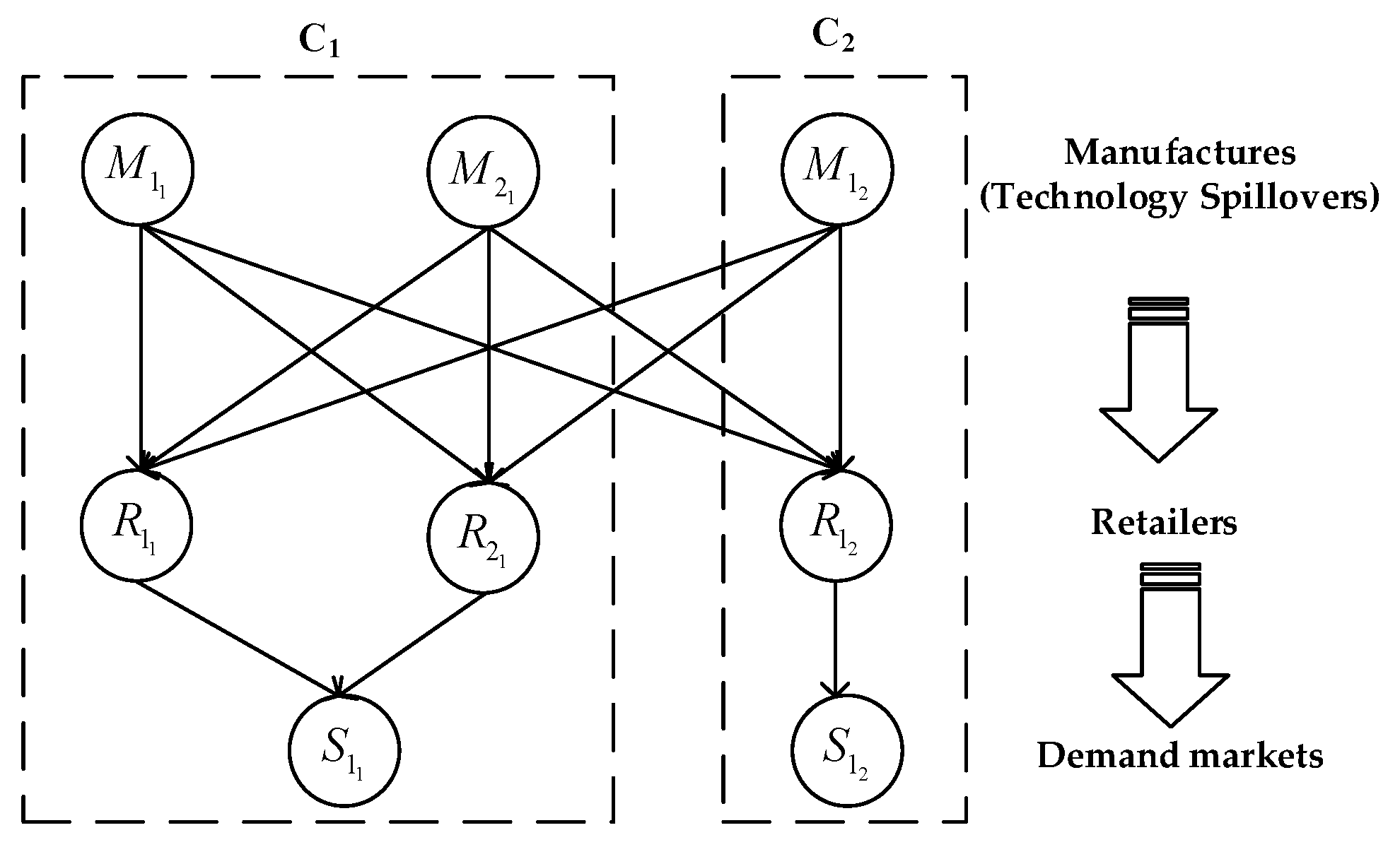
To investigate the effects of R&D subsidies and IPP on various aspects of a global supply chain network in the presence of technology spillover, this study establishes a network involving two countries, three manufacturers, three retailers, and two demand markets. In this network, C₁ comprises two manufacturers, two retailers, and one demand market, while C₂ consists of one manufacturer, one retailer, and one demand market. The products produced by these three manufacturers are perfect substitutes and are distributed to different demand markets through retailers. The structure of this global supply chain network is depicted in Figure 2.

References [1,30] were consulted to establish the relevant cost functions, as shown in

Table 2. Cost functions in the global supply chain network.

Cost Functions	Functional Form
Production cost function	$C_{M_{1_1}}\left(q_{M_{1_1}},L_{M_{1_1}}\right)=0.01q_{M_{1_1}}{}^2+0.01q_{M_{1_1}}\left(q_{M_{2_1}}+q_{M_{1_2}}\right)-0.25L_{M_{1_1}}{q}_{M_{1_1}}$ $C_{M_{2_1}}\left(q_{M_{2_1}},L_{M_{2_1}}\right)=0.01q_{M_{2_1}}{}^2+0.02q_{M_{2_1}}\left(q_{M_{1_1}}+q_{M_{1_2}}\right)-0.25L_{M_{2_1}}{q}_{M_{2_1}}$ $C_{M_{1_2}}\left(q_{M_{1_2}},L_{M_{1_2}}\right)=0.01q_{M_{1_2}}{}^2+0.04q_{M_{1_2}}\left(q_{M_{1_1}}+q_{M_{2_1}}\right)-0.25L_{M_{1_2}}{q}_{M_{1_2}}$
Transaction cost function borne by manufacturers	$C_{M_{1_1}}^{\Omega }\left(q_{M_{1_1}}\right)=0.01q_{M_{1_1}}{}^2+0.1q_{M_{1_1}}$ $C_{M_{2_1}}^{\Omega }\left(q_{M_{2_1}}\right)=0.01q_{M_{2_1}}{}^2+0.1q_{M_{2_1}}$ $C_{M_{1_2}}^{\Omega }\left(q_{M_{1_2}}\right)=0.01q_{M_{1_2}}{}^2+0.1q_{M_{1_2}}$
Technology R&D cost function	$C_{M_{1_1}}^{R\&D}\left({\omega }_{M_{1_1}}\right)=150{\omega }_{M_{1_1}}{}^2$ $C_{M_{2_1}}^{R\&D}\left({\omega }_{M_{2_1}}\right)=180{\omega }_{M_{2_1}}{}^2$ $C_{M_{1_2}}^{R\&D}\left({\omega }_{M_{1_2}}\right)=200{\omega }_{M_{1_2}}{}^2$
Transaction cost function between manufacturers and retailers borne by retailers	$C_{R_{1_1}}^H\left(q_{R_{1_1}}\right)=0.1q_{R_{1_1}}{}^2$ $C_{R_{2_1}}^H\left(q_{R_{2_1}}\right)=0.1q_{R_{2_1}}{}^2$ $C_{R_{1_2}}^H\left(q_{R_{1_2}}\right)=0.1q_{R_{1_2}}{}^2$
Transaction cost function between retailers and markets	$C_{R_{1_1}}^{\Omega }\left(q_{R_{1_1}}\right)=0.05q_{R_{1_1}}{}^2+0.5q_{R_{1_1}}$ $C_{R_{2_1}}^{\Omega }\left(q_{R_{2_1}}\right)=0.05q_{R_{2_1}}{}^2+0.5q_{R_{2_1}}$ $C_{R_{1_2}}^{\Omega }\left(q_{R_{1_2}}\right)=0.05q_{R_{1_2}}{}^2+0.5q_{R_{1_2}}$

. The coefficients of the variables in the cost functions are generally consistent with those in [1,30]. However, to emphasize the research focus of this paper, the differences from these previous works are mainly manifested in the following aspects: These cost functions consider the production cost, which is influenced by transaction volume of the manufacturer itself and its competitors, as well as the technological level (where higher technological levels lead to lower production costs). It is assumed that the manufacturers in C₁ have higher technological levels compared to the manufacturers in C₂. This discrepancy is reflected in the R&D efficiency of the manufacturers, where $M_{1_1}$ exhibits higher R&D efficiency than $M_{2_1}$, and $M_{2_1}$ has higher R&D efficiency than $M_{1_2}$. These distinctions are captured by the coefficients of R&D investment cost, denoted as $C_{M_{1_1}}^{R\&D}\left({\omega }_{M_{1_1}}\right)=150{\omega }_{M_{1_1}}{}^2$, $C_{M_{2_1}}^{R\&D}\left({\omega }_{M_{2_1}}\right)=180{\omega }_{M_{2_1}}{}^2, \mathrm{and} C_{M_{1_2}}^{R\&D}\left({\omega }_{M_{1_2}}\right)=200{\omega }_{M_{1_2}}{}^2$.

5.1. The Impact of Technology Spillovers on Equilibrium Results

In the baseline scenario, the study investigates the impact of technology spillover on equilibrium outcomes, such as R&D technology level, firm profits, and social welfare. In this scenario, the strength of IPP ${\mathsf{\phi }}_M{}_{i_t}$ is set to 0.01, and the technology subsidy $b_{M_{i_t}}$ is set to 0. Social welfare includes firm profits, consumer surplus, and R&D subsidy expenditures, denoted as $SW={{\displaystyle \sum }}_{t=1}^T{{\displaystyle \sum }}_{i=1}^I{\pi }_{M_{i_t}}+{{\displaystyle \sum }}_{t=1}^T{{\displaystyle \sum }}_{j=1}^J{\pi }_{R_{j_t}}+{{\displaystyle \sum }}_{t=1}^T{{\displaystyle \sum }}_{k=1}^K{{\displaystyle \sum }}_{i=1}^I\left({{\displaystyle \int }}_0^{{d_{M_{i_t}}^{S_{k_t}}}^{*}}{p}_{M_{i_t}}^{S_{k_t}}d\left(d_{M_{i_t}}^{S_{k_t}}\right)-{p_{M_{i_t}}^{S_{k_t}}}^{*}{d_{M_{i_t}}^{S_{k_t}}}^{*}\right)-{{\displaystyle \sum }}_{t=1}^T{{\displaystyle \sum }}_{i=1}^I{b}_{i_t}{C}_{M_{i_t}}^{R\&D}\left({\omega }_{M_{i_t}}\right)$ [48]. The total technology level of manufacturers consists of two components: the technology level resulting from their internal R&D investments (R&D technology level) and the technology level derived from external product spillovers. Figure 3 illustrates the relationship between the R&D technology level, the total technology level, and the profits of manufacturers and retailers with respect to the technology spillover. Additionally,

Table 3. Impact of technology spillover on equilibrium results.

$\mathit{\mu }$		$0$	$0.1$	$0.2$	$0.3$	$0.4$	$0.5$	$0.6$	$0.7$	$0.8$	$0.9$	$1$
Wholesale price	$p_{M_{1_1}}$	60.68	60.66	60.64	60.61	60.58	60.55	60.51	60.47	60.43	60.39	60.35
	$p_{M_{2_1}}$	80.12	80.10	80.08	80.06	80.03	80.00	79.96	79.93	79.88	79.84	79.80
	$p_{M_{1_1}}$	120.10	120.09	120.07	120.05	120.03	120.00	119.97	119.93	119.89	119.85	119.81
Retail price	$p_{M_{1_1}}^{S_{1_1}}$	322.47	322.50	322.55	322.59	322.64	322.73	322.78	322.88	322.94	323.00	323.08
	$p_{M_{1_1}}^{S_{1_2}}$	327.26	327.30	327.35	327.38	327.43	327.55	327.58	327.72	327.74	327.81	327.91
	$p_{M_{2_1}}^{S_{1_1}}$	332.93	332.96	333.03	333.05	333.10	333.24	333.26	333.41	333.42	333.48	333.59
	$p_{M_{2_1}}^{S_{1_2}}$	329.23	329.26	329.32	329.35	329.40	329.52	329.55	329.68	329.71	329.77	329.87
	$p_{M_{1_2}}^{S_{1_1}}$	338.38	338.41	338.48	338.50	338.56	338.69	338.71	338.85	338.87	338.93	339.04
	$p_{M_{1_2}}^{S_{1_2}}$	341.31	341.35	341.42	341.43	341.49	341.66	341.65	341.84	341.82	341.87	341.99
Prduction	$q_{M_{1_1}}$	742.87	742.94	742.99	743.09	743.16	743.16	743.27	743.27	743.41	743.50	743.50
	$q_{M_{2_1}}$	757.54	757.61	757.70	757.74	757.81	757.95	757.97	758.12	758.11	758.15	758.23
	$q_{M_{1_2}}$	1500.41	1500.55	1500.69	1500.83	1500.97	1501.11	1501.25	1501.39	1501.52	1501.64	1501.73
SW		294,552.25	294,669.95	294,882.43	294,986.78	295,184.38	295,609.05	295,727.67	296,205.11	296,311.03	296,555.41	296,926.53

demonstrates the relationship between wholesale price, retail price, production volume, and technology spillover.

From Figure 3a,b, it can be observed that as the technology spillover increases, the R&D technology level of manufacturers also increases. $M_{1_1}$, with higher R&D efficiency, experiences a faster rate of R&D investment growth compared to $M_{2_1}$ and $M_{1_2}$, which have lower R&D efficiency and rely more on technology-level improvements from spillover. Furthermore, technology spillovers enhance the technology levels of manufacturers and reduce production costs, leading to a decrease in wholesale prices for the products. Simultaneously, the increased technology levels influence consumer demand, resulting in higher retail prices for the products (as shown in Table 3).

5.2. The Impact of R&D Subsidies on Equilibrium Results

This section examines the impact of subsidy forms and sizes on the equilibrium results when different governments simultaneously adopt R&D subsidy policies. Two types of subsidies are considered: symmetric subsidies, where different countries provide the same subsidy rate for their manufacturers’ R&D investment, and asymmetric subsidies, where different countries offer different subsidy rates.

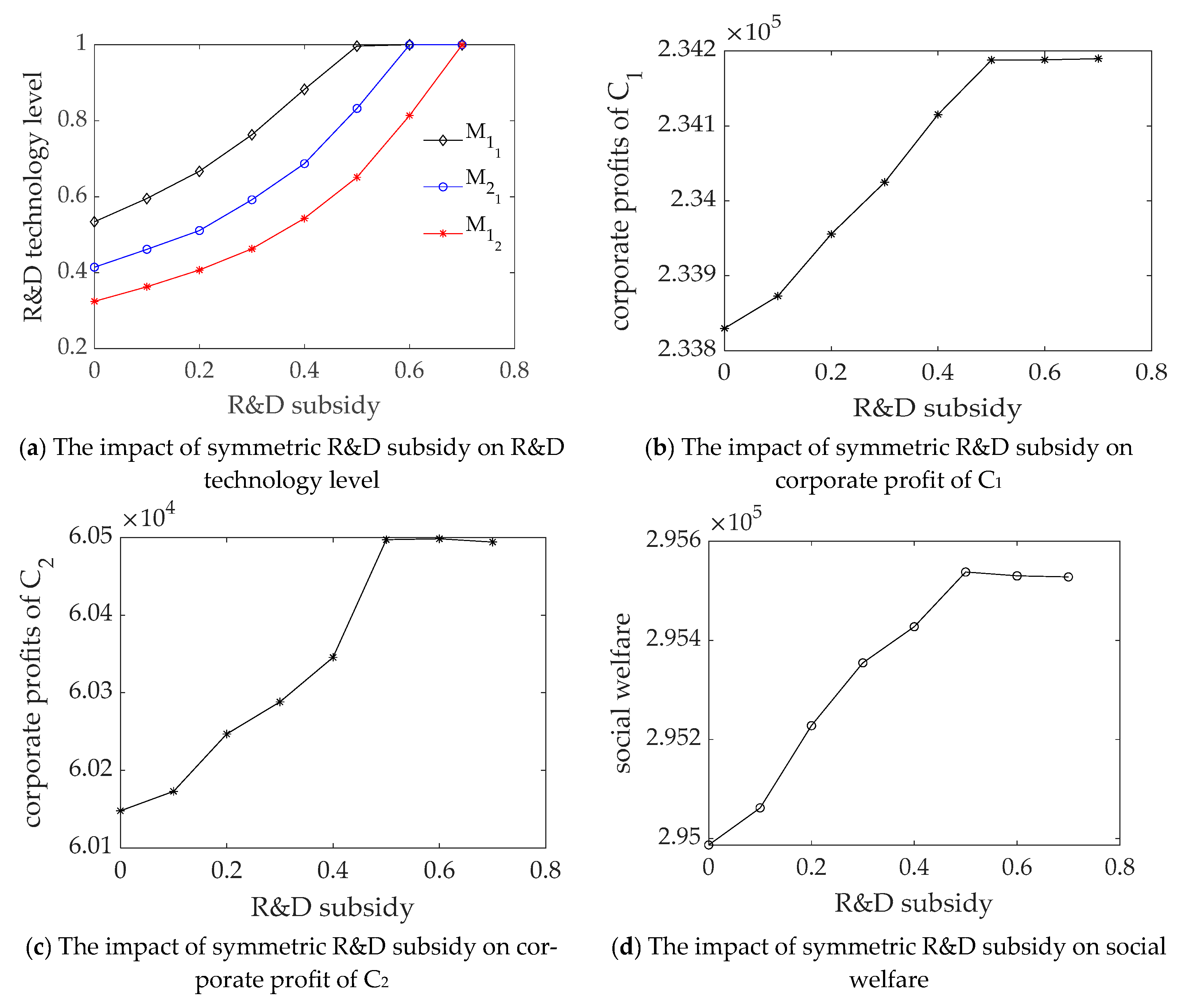
Case 1: Impact of symmetric R&D subsidy on equilibrium results

In this situation, the intensity of IPP is ${\mathsf{\phi }}_M{}_{i_t}=0.01$, and the technology spillover rate is μ = 0.3. The relationship between manufacturers’ technological levels and their profits, retailers’ profits, social welfare, and subsidy rates is depicted in Figure 4.

From Figure 4, it is evident that under symmetric subsidies, the R&D technology level of manufacturers increases as the subsidy rate rises. However, when the subsidy rate reaches 0.5, the R&D technology level of $M_{1_1}$ reaches its maximum level, and the effectiveness of the subsidy starts to diminish. At this point, the total profits of manufacturers in C₁ and C₂ no longer increase, and the benefits of the subsidy become outweighed by subsidy expenditure, leading to a decline in social welfare.

By examining

Table 4. The relationship between subsidy and price and production under symmetrical subsidy.

${\mathit{b}}_{{\mathit{M}}_{{\mathit{i}}_{\mathit{t}}}}$		0	0.1	0.2	0.3	0.4	0.5	0.6
Wholesale price	$p_{M_{1_1}}$	60.61	60.60	60.58	60.56	60.53	60.50	60.49
	$p_{M_{2_1}}$	80.06	80.05	80.04	80.02	80.00	79.97	79.93
	$p_{M_{1_1}}$	120.05	120.04	120.04	120.03	120.02	120.00	119.97
Retail price	$p_{M_{1_1}}^{S_{1_1}}$	322.59	322.61	322.65	322.69	322.73	322.80	322.80
	$p_{M_{1_1}}^{S_{1_2}}$	327.38	327.40	327.44	327.47	327.51	327.59	327.61
	$p_{M_{2_1}}^{S_{1_1}}$	333.05	333.07	333.11	333.14	333.18	333.28	333.28
	$p_{M_{2_1}}^{S_{1_2}}$	329.35	329.37	329.41	329.45	329.49	329.58	329.58
	$p_{M_{1_2}}^{S_{1_1}}$	338.50	338.52	338.57	338.61	338.65	338.75	338.77
	$p_{M_{1_2}}^{S_{1_2}}$	341.43	341.45	341.51	341.54	341.57	341.69	341.69
Production	$q_{M_{1_1}}$	743.09	743.14	743.17	743.25	743.35	743.42	743.56
	$q_{M_{2_1}}$	757.74	757.78	757.86	757.93	758.02	758.18	758.26
	$q_{M_{1_2}}$	1500.83	1500.92	1501.03	1501.18	1501.37	1501.61	1501.82

, it can be observed that the subsidy reduces the production costs for manufacturers, resulting in lower wholesale prices. However, the increase in technology level also intensifies competition among manufacturers. Furthermore, the subsidy stimulates improvements in technology levels, leading to an increase in retail prices, which somewhat undermines consumer interests.

Case 2: The impact of asymmetric R&D subsidies on equilibrium results

In this scenario, two scenarios are considered: Scenario I with a subsidy rate of 0.3 in C₁ and 0.1 in C₂, and Scenario II with a subsidy rate of 0.1 in C₁ and 0.3 in C₂. Other parameters remain unchanged. The equilibrium decisions and social welfare under different scenarios are presented in

Table 5. Equilibrium decision results under asymmetric subsidy policies.

		Scenario I	Scenario II
R&D technology level	${\omega }_{M_{1_1}}$	0.7625	0.5966
	${\omega }_{M_{2_1}}$	0.5898	0.4618
	${\omega }_{M_{1_2}}$	0.3627	0.4604
Wholesale price	$p_{M_{1_1}}$	60.5594	60.5946
	$p_{M_{2_1}}$	80.0219	80.0479
	$p_{M_{1_2}}$	120.0481	120.0244
Retail price	$p_{M_{1_1}}^{S_{1_1}}$	322.6799	322.6169
	$p_{M_{1_1}}^{S_{1_2}}$	327.4532	327.4127
	$p_{M_{2_1}}^{S_{1_1}}$	333.1125	333.0934
	$p_{M_{2_1}}^{S_{1_2}}$	329.4376	329.3813
	$p_{M_{1_2}}^{S_{1_1}}$	338.6066	338.5242
	$p_{M_{1_2}}^{S_{1_2}}$	341.5091	341.4774
Production	$q_{M_{1_1}}$	743.2241	743.1574
	$q_{M_{2_1}}$	757.8880	757.8276
	$q_{M_{1_2}}$	1501.1121	1500.9849
Manufacturer’s profit	${\pi }_{M_{1_1}}$	20,832.8702	20,839.2603
	${\pi }_{M_{2_1}}$	20,089.6397	20,092.0412
	${\pi }_{M_{1_2}}$	19,058.6739	19,055.7499
Retailer’s profit	${\widehat{\pi }}_{R_{1_1}}$	93,415.1350	93,360.8373
	${\widehat{\pi }}_{R_{2_1}}$	99,651.7727	99,614.8874
	${\widehat{\pi }}_{R_{1_2}}$	41,222.2231	41,126.1401
Social welfare	SW	295,322.0579	295,094.8394
Firms’ profits within C1		233,989.4175	233,907.0263
Firms’ profits within C2		60,280.8970	60,181.8900

.

From Table 5, it can be observed that under asymmetric subsidies policies, countries with higher subsidy rates experience a greater increase in R&D technology investment compared to non-subsidy scenarios ($b_{M_{i_t}}=0$). This indicates that both symmetric and asymmetric subsidies can effectively enhance the R&D technology levels of manufacturers. Comparing Scenarios I and II, it is evident that Scenario I leads to higher retail prices, production quantities, retailers’ profits, social welfare, and corporate profits for country C1. However, the wholesale prices and profits of $M_{1_1}$ and $M_{2_1}$ exhibit an opposite trend. This indicates that when a country adopts asymmetric subsidies, for high-tech countries (C1), a high subsidy is beneficial to the profits of its retailers and social welfare, but the cost is the sacrifice of its manufacturers.

5.3. The Impact of IPP on Equilibrium Results

IPP is closely related to the technological R&D of enterprises. Therefore, studying the impact of IPP intensity on the R&D investment level, product prices, enterprise profits, and social welfare in the global supply chain network is of great significance. Similarly, in this section, we discuss two cases: symmetric IPP strength and asymmetric IPP strength.

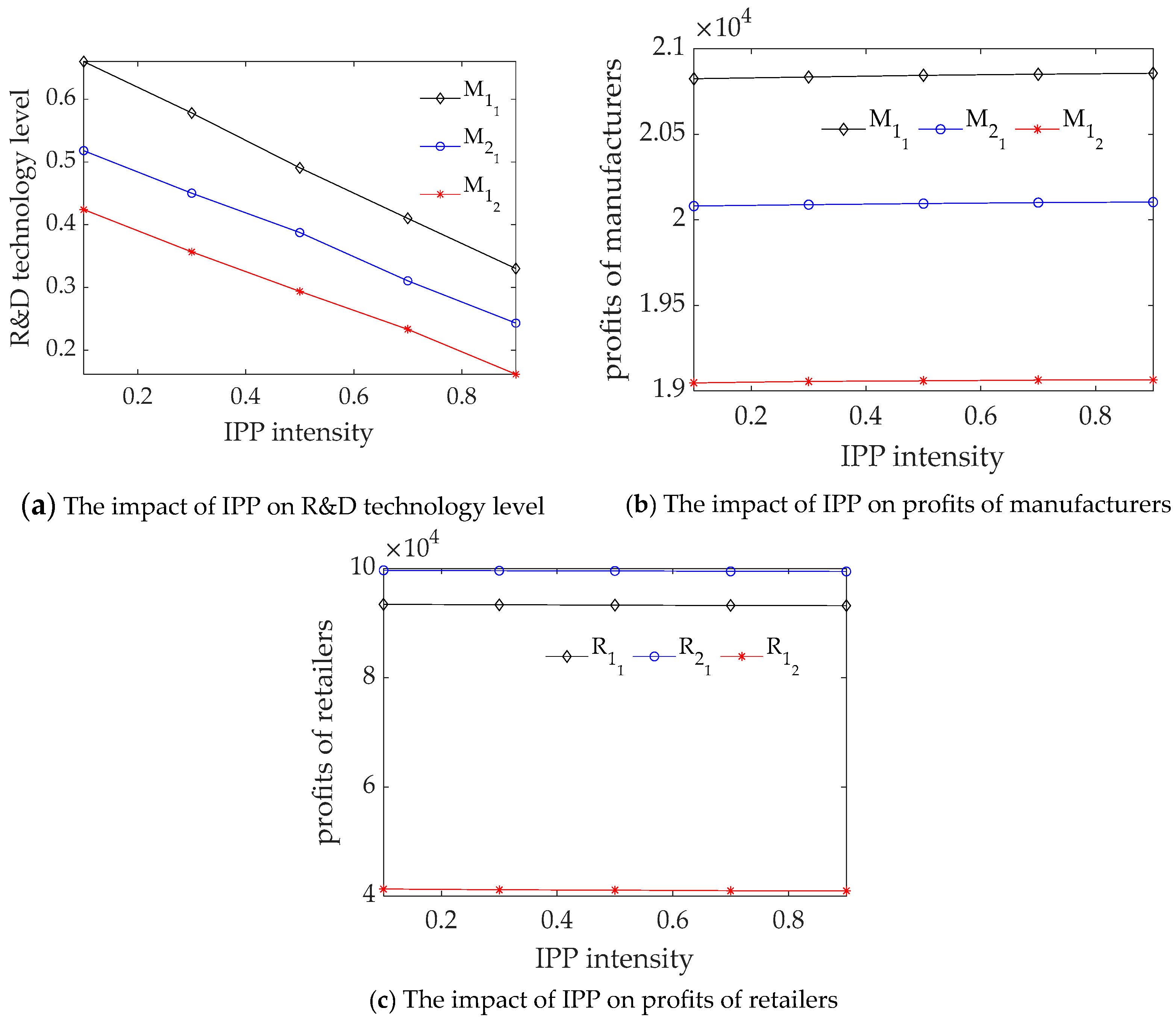
Case 1: Impact of symmetrical IPP policy on equilibrium results

To better observe the effects of IPP, let us assume that the government does not provide any R&D subsidies to manufacturers. In this case, the technological spillover rate for manufacturers is μ = 0.5, and all other parameters remain consistent. The relationship between the R&D technology level, manufacturer and retailer profits, and the strength of IPP is illustrated in Figure 5 and

Table 6. Equilibrium results under symmetric IPP.

The Strength of IPP		$\mathit{\phi }=0.1$	$\mathit{\phi }=0.3$	$\mathit{\phi }=0.5$	$\mathit{\phi }=0.7$	$\mathit{\phi }=0.9$
Wholesale price	$p_{M_{1_1}}$	60.56	60.59	60.63	60.65	60.67
	$p_{M_{2_1}}$	80.02	80.05	80.07	80.09	80.11
	$p_{M_{1_2}}$	120.01	120.04	120.06	120.08	120.09
Retail price	$p_{M_{1_1}}^{S_{1_1}}$	322.68	322.62	322.58	322.52	322.49
	$p_{M_{1_1}}^{S_{1_2}}$	327.49	327.41	327.38	327.31	327.30
	$p_{M_{2_1}}^{S_{1_1}}$	333.16	333.08	333.05	332.98	332.97
	$p_{M_{2_1}}^{S_{1_2}}$	329.45	329.38	329.35	329.28	329.26
	$p_{M_{1_2}}^{S_{1_1}}$	338.61	338.53	338.50	338.43	338.42
	$p_{M_{1_2}}^{S_{1_2}}$	341.55	341.46	341.44	341.37	341.36
Production	$q_{M_{1_1}}$	743.17	743.12	743.03	742.98	742.88
	$q_{M_{2_1}}$	757.87	757.78	757.73	757.64	757.59
	$q_{M_{1_2}}$	1501.04	1500.90	1500.76	1500.62	1500.48
Manufacturer’s profit	${\pi }_{M_{1_1}}$	20,825.18	20,835.28	20,845.82	20,851.64	20,857.11
	${\pi }_{M_{2_1}}$	20,081.23	20,089.40	20,095.38	20,101.20	20,104.32
	${\pi }_{M_{1_2}}$	19,047.69	19,055.66	19,059.78	19,063.68	19,065.04
Retailer’s profit	${\widehat{\pi }}_{R_{1_1}}$	93,431.95	93,357.32	93,308.01	93,248.66	93,215.94
	${\widehat{\pi }}_{R_{2_1}}$	99,688.74	99,601.87	99,562.05	99,491.16	99,466.98
	${\widehat{\pi }}_{R_{1_2}}$	41,282.54	41,136.07	41,087.43	40,974.60	40,957.55

.

Observing Figure 5, it becomes evident that as the intensity of IPP increases, there is a discernible decline in the R&D technology level and the profits of retailers. Conversely, manufacturer profits experience an upward trajectory. Furthermore, referring to Table 6, it can be observed that higher IPP leads to an increase in wholesale prices and manufacturer profits. However, there is a slight decrease in the quantity produced, accompanied by a decrease in both retail prices and retailer profits.

Case 2: The impact of asymmetric IPP on global supply chain networks

In this section, the article mainly focuses on the impact of IPP intensity on firms’ profits, technological levels, and social welfare. In Scenario I, C₁ has an IPP intensity of 0.5, while C₂ has an intensity of 0.3. In Scenario II, C₁ has an intensity of 0.3, while C₂ has an intensity of 0.5. Other parameters remain consistent with Case 1. The equilibrium results obtained are shown in

Table 7. Equilibrium results under asymmetric IPP policies.

		Scenario I	Scenario II
R&D technology level	${\omega }_{M_{1_1}}$	0.5329	0.5395
	${\omega }_{M_{2_1}}$	0.4160	0.4164
	${\omega }_{M_{1_2}}$	0.2952	0.3573
Wholesale price	$p_{M_{1_1}}$	60.6171	60.6037
	$p_{M_{2_1}}$	80.0641	80.0530
	$p_{M_{1_2}}$	120.0492	120.0489
Retail price	$p_{M_{1_1}}^{S_{1_1}}$	322.6002	322.6003
	$p_{M_{1_1}}^{S_{1_2}}$	327.4134	327.3882
	$p_{M_{2_1}}^{S_{1_1}}$	333.0985	333.0501
	$p_{M_{2_1}}^{S_{1_2}}$	329.3784	329.3575
	$p_{M_{1_2}}^{S_{1_1}}$	338.5359	338.5151
	$p_{M_{1_2}}^{S_{1_2}}$	341.4999	341.4381
Production	$q_{M_{1_1}}$	743.0240	743.1026
	$q_{M_{2_1}}$	757.7829	757.7489
	$q_{M_{1_2}}$	1500.8068	1500.8515
Manufacturer’s profit	${\pi }_{M_{1_1}}$	20,842.2260	20,839.7405
	${\pi }_{M_{2_1}}$	20,092.5104	20,093.5001
	${\pi }_{M_{1_2}}$	19,059.2996	19,055.0483
Retailer’s profit	${\widehat{\pi }}_{R_{1_1}}$	93,335.2745	93,337.1849
	${\widehat{\pi }}_{R_{2_1}}$	99,602.5924	99,576.1128
	${\widehat{\pi }}_{R_{1_2}}$	41,154.9177	41,104.9414
Social welfare	SW	295,095.8970	295,015.9036
Firms’ profits within C1		233,872.6032	233,846.5383
Firms’ profits within C2		60,214.2174	60,159.9896

.

Based on the analysis presented in Table 7, the following conclusions can be drawn: Compared to Scenario II, Scenario I exhibits a lower R&D technology level. However, Scenario I demonstrates higher wholesale prices, retail prices, profits for C₁ and C₁, as well as social welfare, when compared to Scenario II. Therefore, the analysis indicates that when two countries adopt asymmetric IPP policies, a higher IPP implemented by the high-tech country (C₁) leads to a decrease in the R&D technology level but has positive effects on profits and social welfare.

Chen et al. [49], in a study that is relevant to this article, established a supply chain comprising a single manufacturer and a single retailer to investigate the green R&D decisions of manufacturers and retailers under different ownership structures, as well as the ramifications of R&D decisions on the supply chain. The article assumes that technology spillovers occur between upstream and downstream entities and that technology can lead to emission reduction. However, in reality, technology spillover is typically observed among enterprises at the same level, and technological advancements can lower production costs. Furthermore, Hao et al. [9] conducted an empirical analysis to explore the influence of technology spillovers on carbon emissions while considering the constraints of IPP policies. This study characterizes technology spillovers at the macro level and does not delve into the impact of intellectual property protection policies from the perspective of global supply chain networks. In comparison, our article references the technology R&D investment cost function from [49] and examines the effects of technology spillovers among enterprises at the same level, as well as the combined impacts of R&D subsidies and IPP, on the equilibrium decision making and social welfare of global supply chain network members.

5.4. Managerial and Policy Implications

This study provides important insights into the equilibrium decision making of members within the global supply chain under different technology spillovers, R&D subsidies, and IPP policies. From a national perspective, when formulating R&D subsidies and IPP policies, policymakers need to consider not only relevant policies in other countries but also the technological R&D levels of domestic manufacturers and the rate of technology spillover among enterprises, in order to develop appropriate R&D subsidies and IPP policies because, under asymmetric subsidy policies, high-tech-level countries’ governments, adopting high subsidy rates, may risk undermining the profitability of their manufacturers. For retailers, technology spillover and R&D subsidies have positive effects, while IPP has a negative impact. Consequently, retailers may seek to increase the rate of technology spillover among manufacturers and request higher R&D subsidies while reducing the strength of IPP measures. However, for manufacturers, higher R&D investments and technological levels do not necessarily lead to better outcomes, and they must simultaneously consider government R&D subsidies, IPP policies, and the rate of technology spillover among enterprises.

6. Conclusions

This paper investigates the influence of R&D subsidies and IPP on the equilibrium decision making in global supply chain networks, considering the context of technology spillover. Firstly, by applying the Nash equilibrium and variational inequalities theory, optimal decisions and equilibrium conditions are derived for manufacturers, retailers, and demand markets. Secondly, through the analysis of equilibrium results under various scenarios, the following conclusions are drawn:

As the technology spillover rate increases, the derived R&D technology level improves. Moreover, manufacturers with higher R&D efficiency experience a more rapid increase in their technological levels. However, the intensifying competition resulting from improved technological levels may have a negative impact on manufacturers’ profits.

Under symmetric subsidy policies, as the subsidy rate increases, manufacturers’ R&D investment tends to increase. However, the effectiveness of the subsidy diminishes, resulting in no further increase in total profits and even a decline, thereby negatively affecting social welfare. Under asymmetric subsidy policies, providing higher subsidies to high-tech countries benefits the profits of retailers and contributes to social welfare, but it may harm the interests of manufacturers in high-tech countries.

Under symmetric IPP policies, as the protection intensity increases, manufacturers’ R&D investment and retailer profits decrease, while manufacturer profits increase. Under asymmetric IPP policies, when high-tech countries adopt higher levels of IPP, it leads to a decrease in the R&D investment level of manufacturers. However, it has a positive impact on retailer profits and overall social welfare.

The contribution of this study lies in the following aspects: Firstly, it explores the impact of government R&D subsidies and IPP policies on the equilibrium decisions of enterprises within the global supply chain network. Secondly, by setting up a benchmark, it examines the effects of symmetric and asymmetric R&D subsidies and IPP on firm profits and social welfare. This contributes to a deeper understanding of the interaction mechanisms of R&D subsidies and IPP within the context of the global supply chain network.

However, while this study provides a decision-making basis for governments and supply chain members, it does have certain limitations that should be addressed in future research. Firstly, in the context of a multipolar global economy, trade frictions are bound to arise. Future studies could benefit from incorporating the risks associated with firms’ technology R&D and exploring the equilibrium decision making of governments and firms in the presence of such risks. Secondly, this study focused solely on horizontal technology spillover, while, in reality, both horizontal and vertical technology spillovers often coexist. Therefore, future research should aim to simultaneously consider both types of technology spillovers.