
Offset Optimization Model for Signalized Intersections Considering the Optimal Location Planning of Bus Stops

Abstract
1. Introduction
2. Optimization Model
2.1. Notations Description
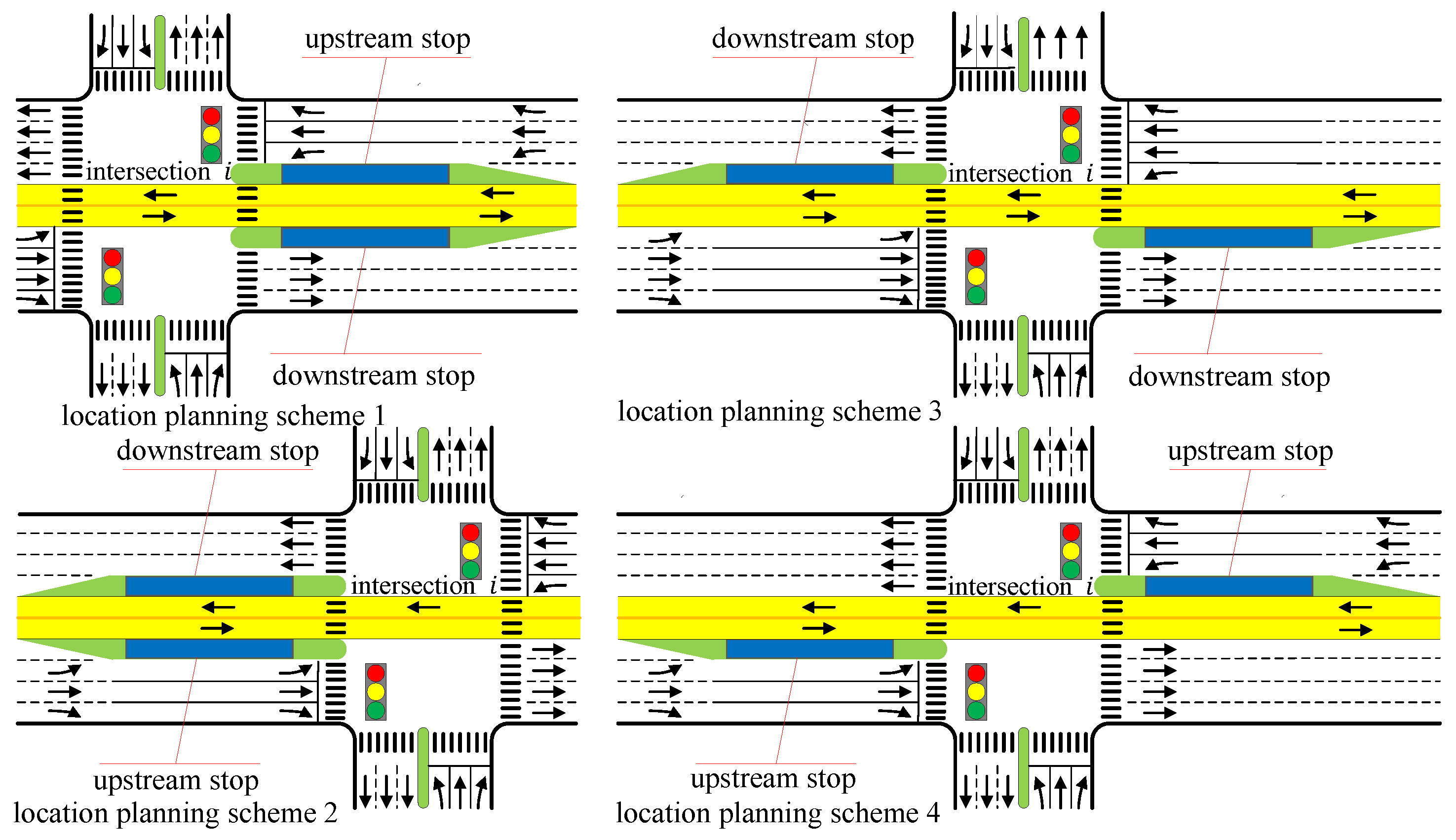
2.2. Decision Variables
2.3. Objective Function
2.4. Problem Constraints
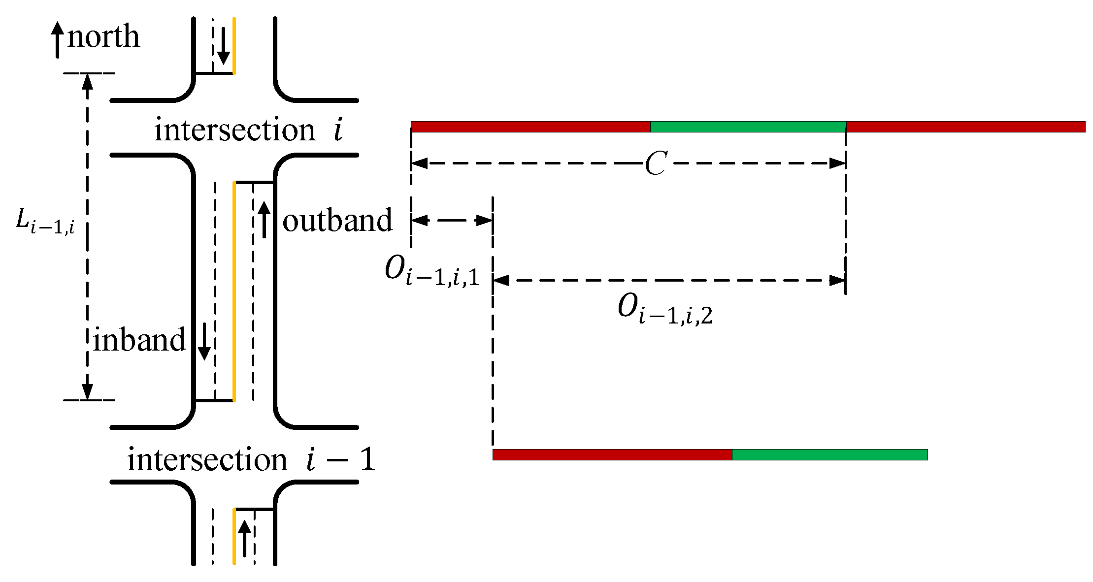
2.4.1. Offset Constraints
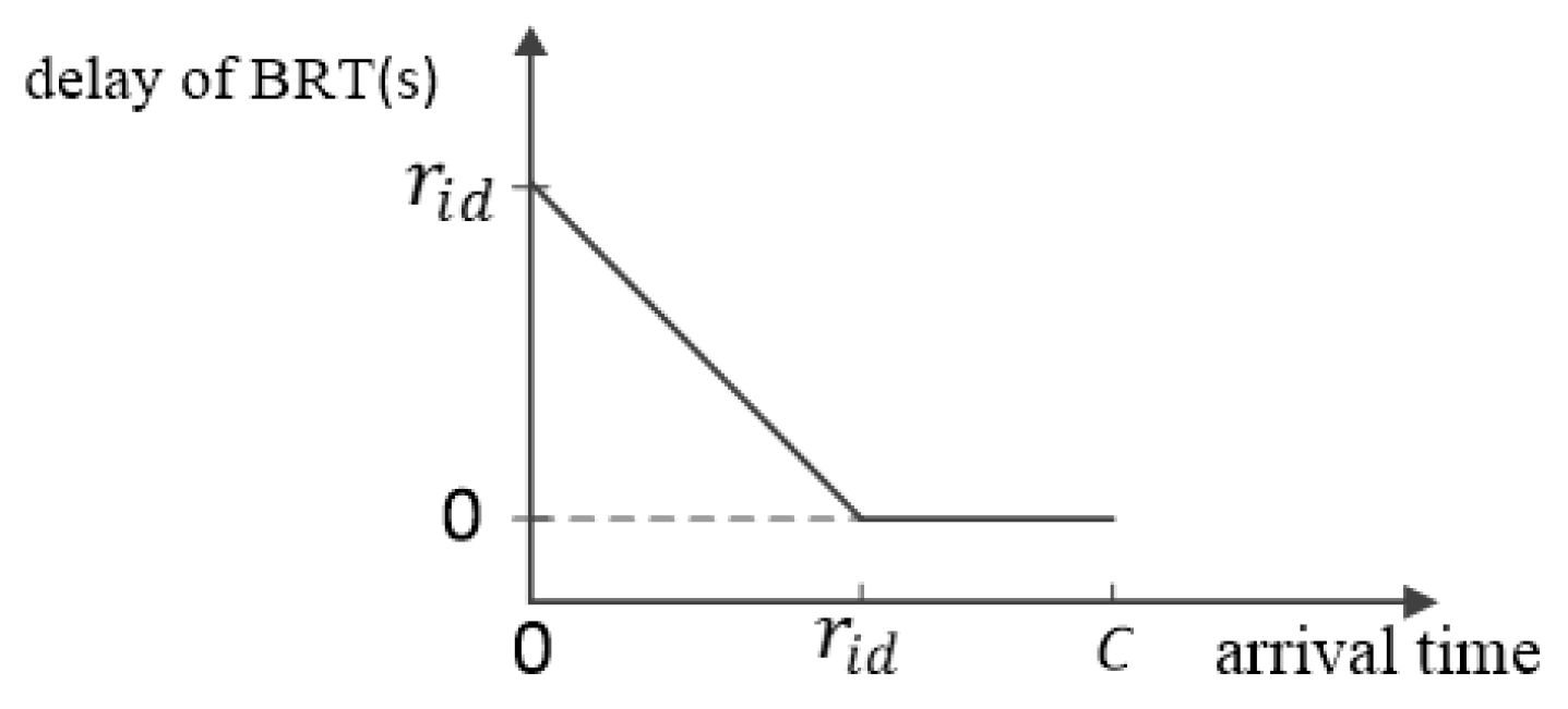
2.4.2. Prediction of BRT Delays
- (i)
- The delay characteristics of BRT
- (ii)
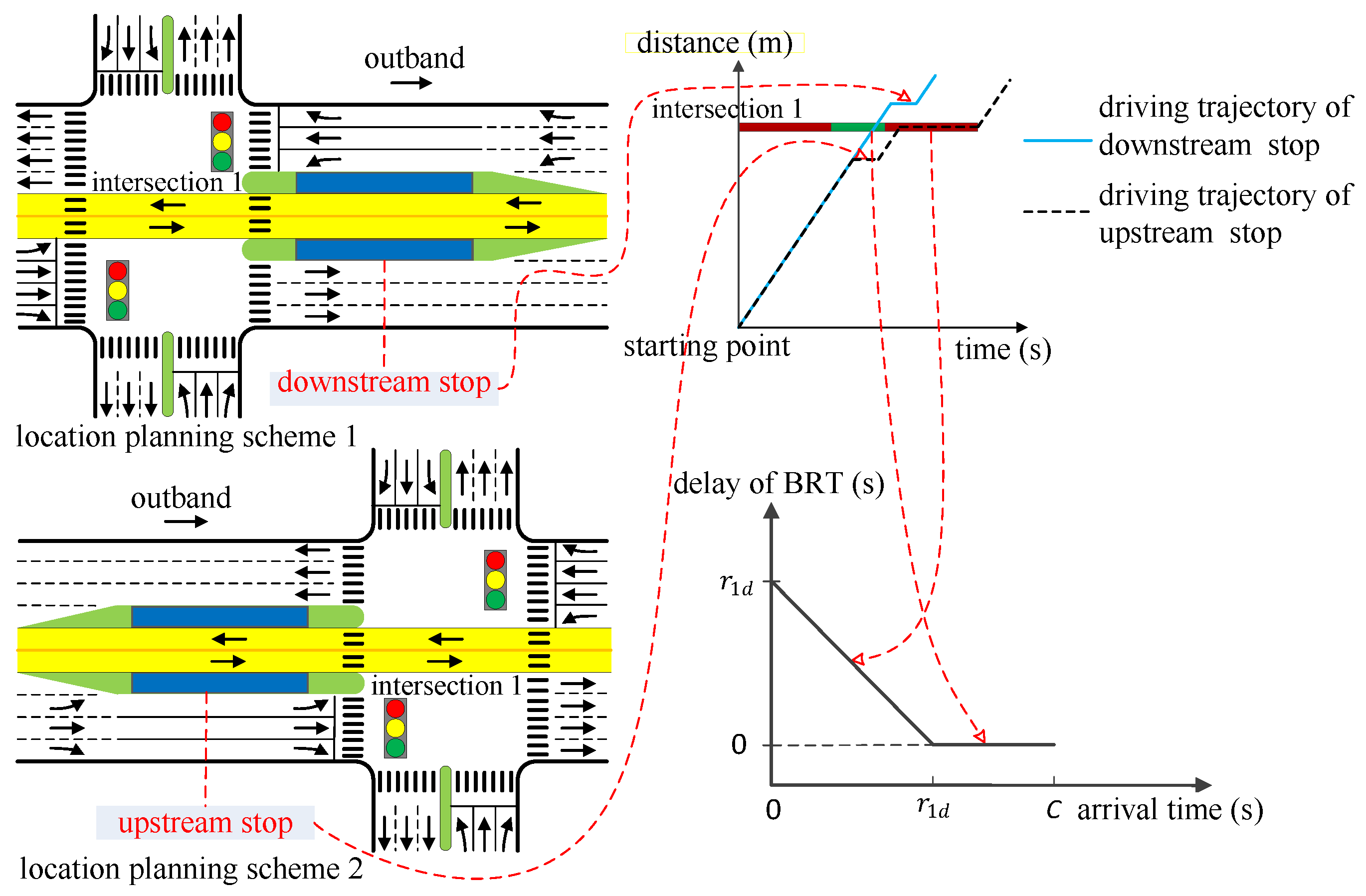
- BRT delay at the starting intersection
- (iii)
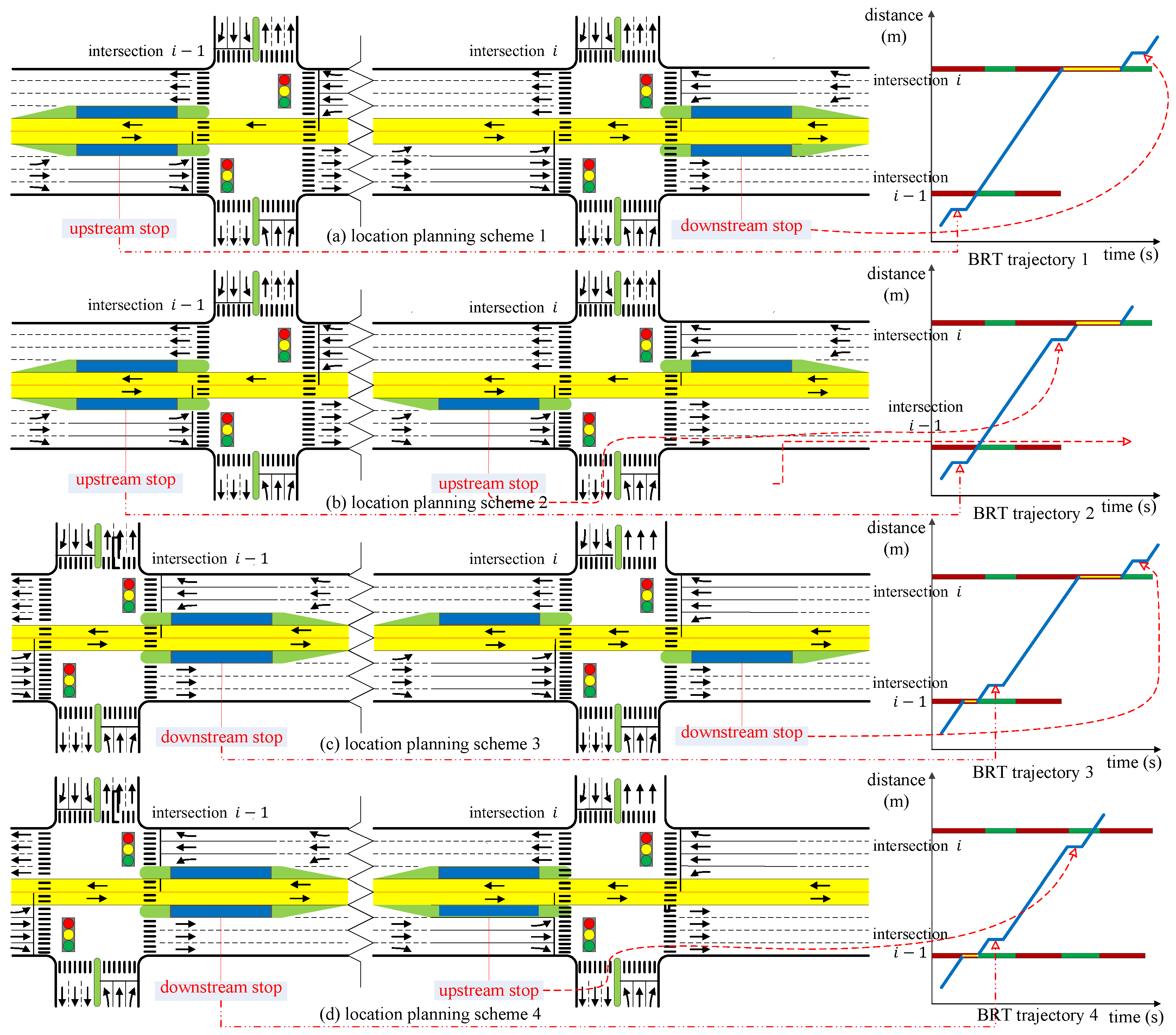
- BRT delay at the other intersections
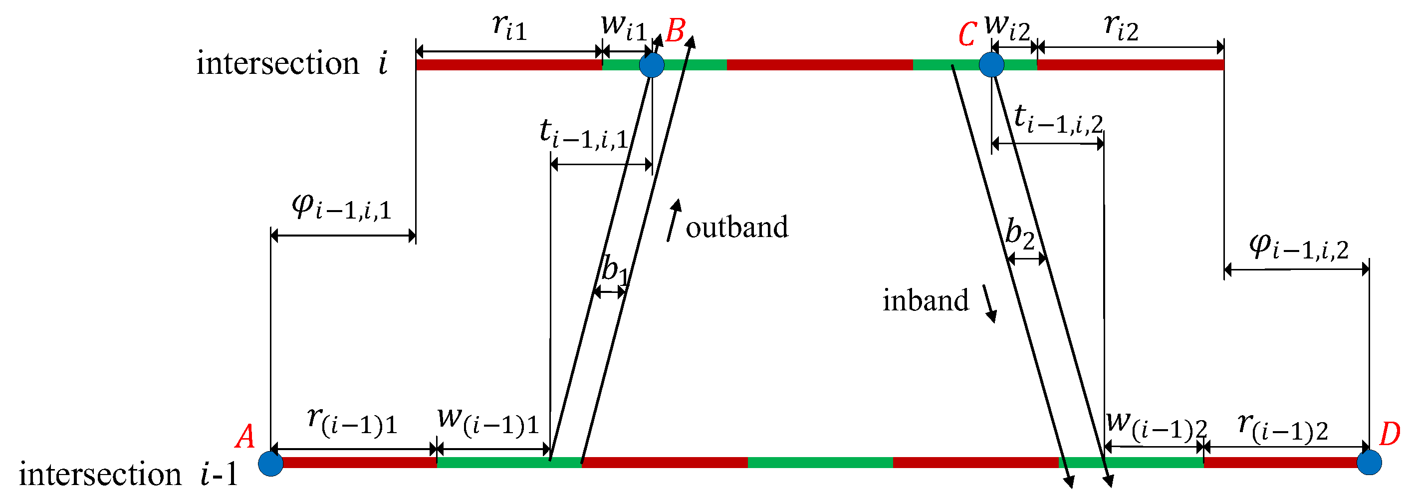
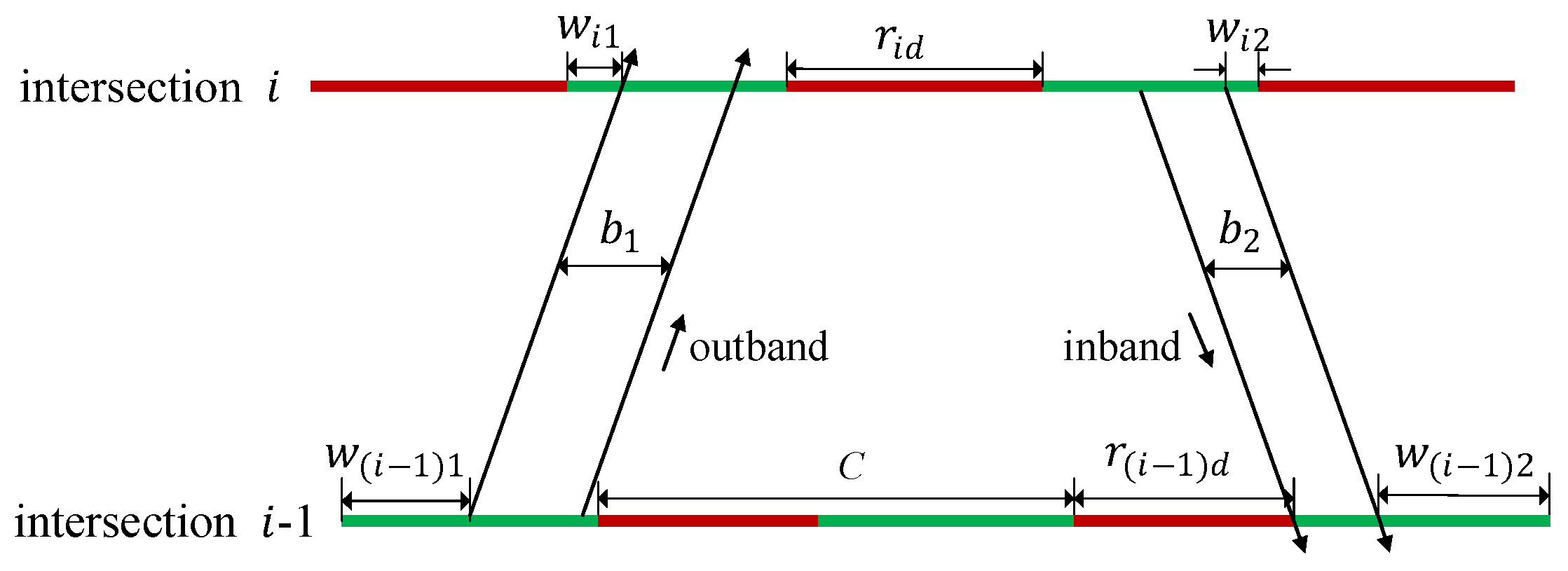
2.4.3. Green Wave Bandwidth of Cars
3. Solving the Model
3.1. Linearization of the Rounding Function
3.2. Linearization of the Piecewise Functions
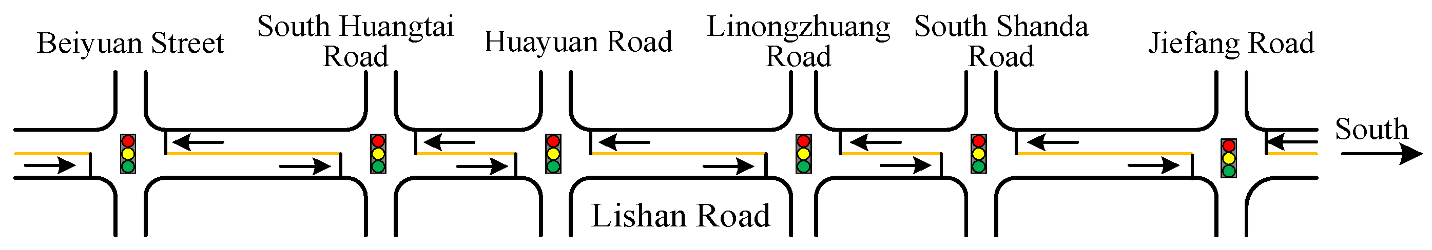
4. Case Study
4.1. Parameter Input
4.2. Comparison and Analysis
4.2.1. Scheme Comparison
4.2.2. Results Analysis
- (i)
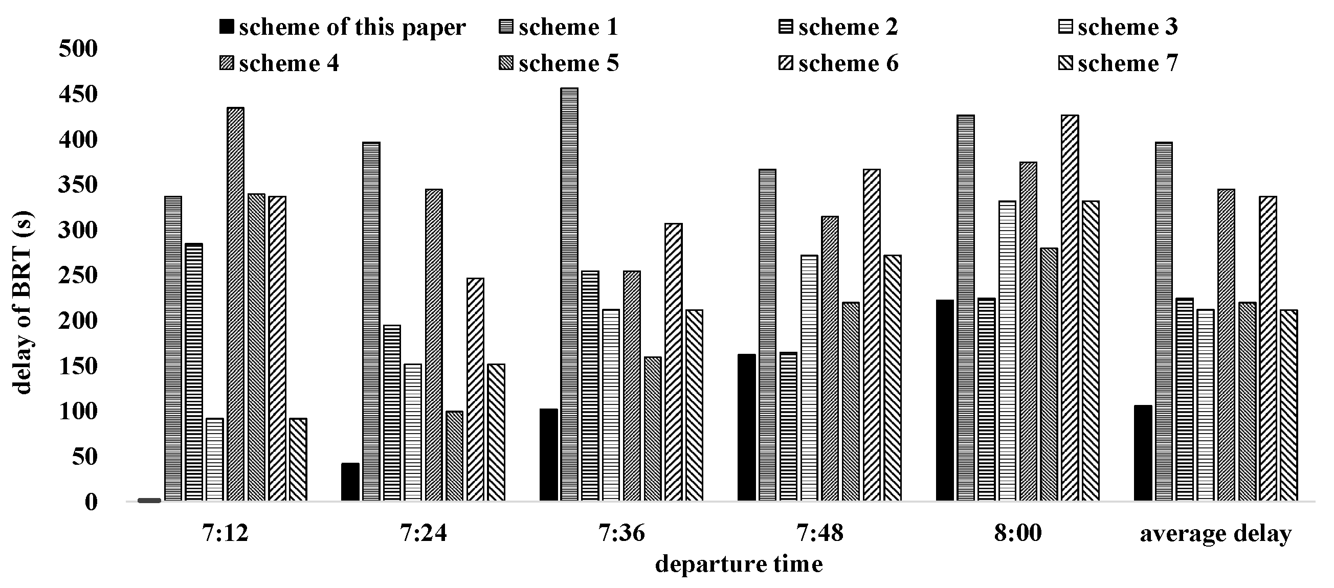
- Analysis of BRT delays
- (ii)
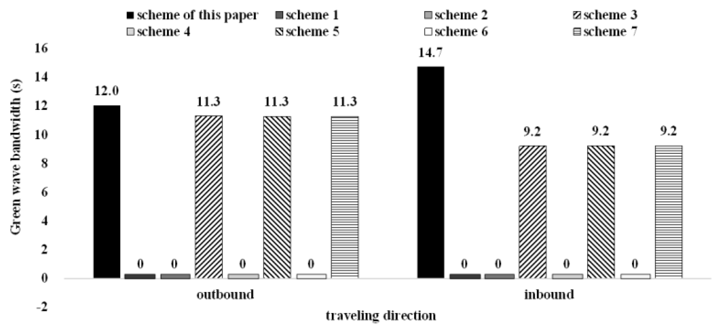
- Bandwidth analysis of cars
5. Sensitivity Analysis
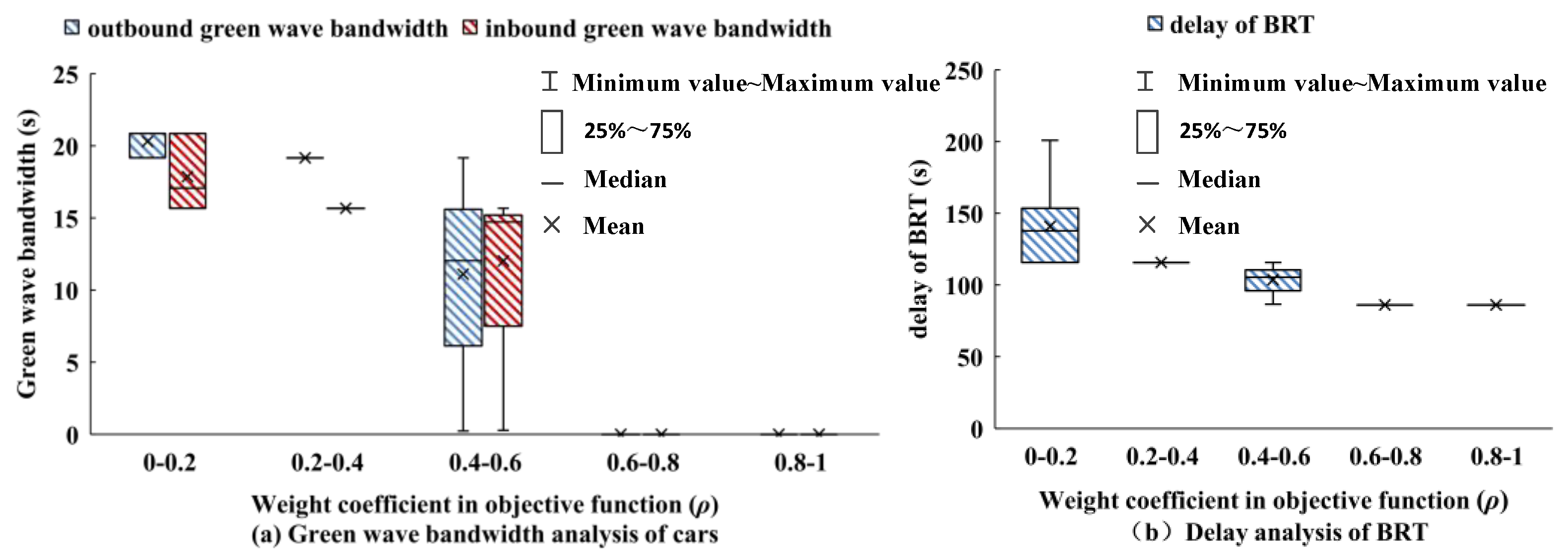
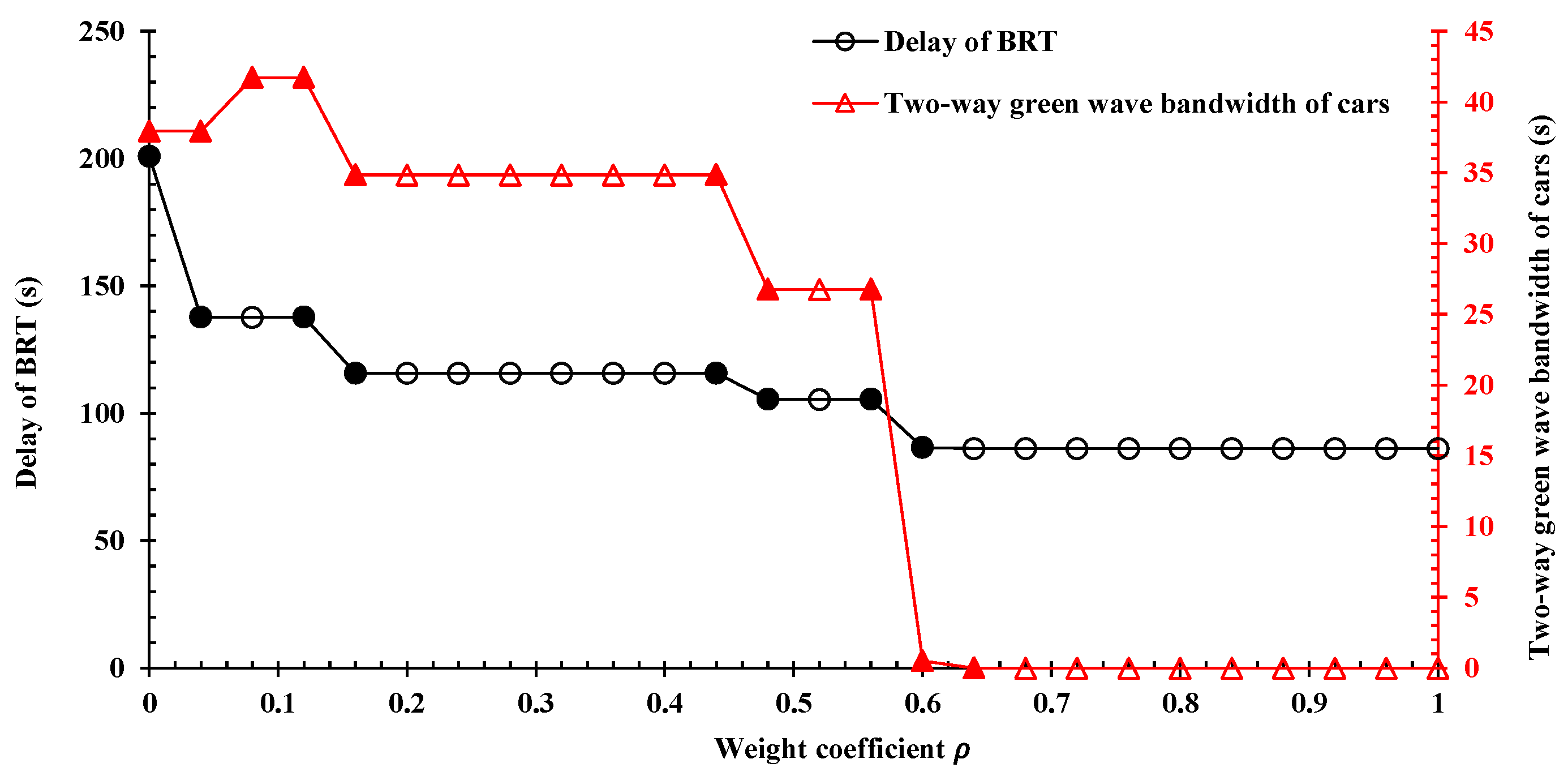
5.1. Weight Coefficient
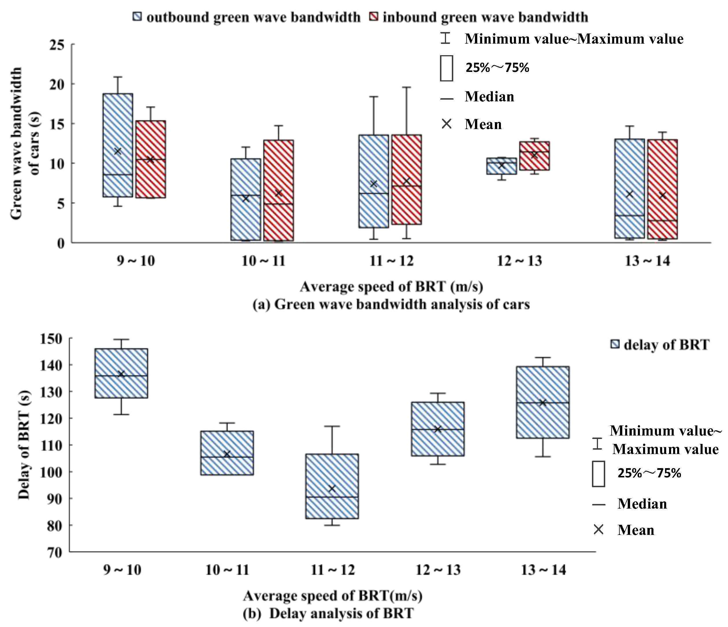
5.2. BRT-Vehicle Speed
6. Conclusions
Author Contributions
Funding
Data Availability Statement
Conflicts of Interest
References
- Cao, M.; Yang, C. Research on Consumer Identity in Using Sustainable Mobility as a Service System in a Commuting Scenario. Systems 2022, 10, 223. [Google Scholar] [CrossRef]
- Sun, Y.D.; Jiang, J.Y.; Lam, S.K.; He, P.L. Learning traffic network embeddings for predicting congestion propagation. IEEE Trans. Intell. Transp. Syst. 2022, 23, 11591–11604. [Google Scholar] [CrossRef]
- Wu, W.; Ma, W.; Long, K.; Wang, Y. Integrated Optimization of Bus Priority Operations in Connected Vehicle Environment. J. Adv. Transp. 2016, 50, 1573–2337. [Google Scholar] [CrossRef]
- Mylonakou, M.; Chassiakos, A.; Karatzas, S.; Liappi, G. System Dynamics Analysis of the Relationship between Urban Transportation and Overall Citizen Satisfaction: A Case Study of Patras City, Greece. Systems 2023, 11, 112. [Google Scholar] [CrossRef]
- Li, M.; Boriboonsomsin, K.; Wu, G.Y.; Zhang, W.B. Traffic energy and emission reductions at signalized intersections: A study of the benefits of advanced driver information. Int. J. Intell. Transp. Syst. Res. 2009, 7, 2327–2332. [Google Scholar]
- Schrank, D.; Albert, L.; Eisele, B.; Lomax, T. 2021 Urban Mobility Report; The Texas A&M Transportation Institute: Bryan, TX, USA; INRIX: Kirkland, WA, USA, 2021. [Google Scholar]
- Chen, J.X.; Wang, S.A.; Liu, Z.Y.; Chen, X.W. Network-level optimization of bus stop placement in urban areas. KSCE J. Civ. Eng. 2018, 22, 1446–1453. [Google Scholar] [CrossRef]
- Wu, W.; Larry, H.; Yan, S.H.Y.; Ma, W.J. Development and evaluation of bus lanes with intermittent and dynamic priority in connected vehicle environment. J. Intell. Transp. Syst. 2018, 22, 301–310. [Google Scholar] [CrossRef]
- AlRukaibi, F.; AlKheder, S. Optimization of bus stop stations in Kuwait. Sustain. Cities Soc. 2019, 44, 726–738. [Google Scholar] [CrossRef]
- Cvitanic, D. Joint impact of bus stop location and configuration on intersection performance. Promet-Traffic Transp. 2017, 29, 443–454. [Google Scholar] [CrossRef]
- Diab, E.I.; EI-Geneidy, A.M. The farside story measuring the benefits of bus stop location on transit performance. Transp. Res. Rec. 2015, 2538, 1–10. [Google Scholar] [CrossRef]
- Cui, Y.; Chen, S.K.; Liu, J.F.; Jia, W.Z. Optimal locations of bus stops connecting subways near urban intersections. Math. Probl. Eng. 2015, 2015, 1563–5147. [Google Scholar] [CrossRef]
- Furth, P.G.; SanClemente, J.L. Near Side, Far Side, Uphill, Downhill: Impact of Bus Stop Location on Bus Delay. Transp. Res. Rec. J. Transp. Res. Board 2006, 1971, 66–73. [Google Scholar] [CrossRef]
- Tirachini, A. The economics and engineering of bus stops: Spacing, design and congestion. Transp. Res. Part A Policy Pract. 2014, 59, 37–57. [Google Scholar] [CrossRef]
- Medina, M.; Giesen, R.; Muñoz, J.C. Model for the optimal location of bus stops and its application to a public transport corridor in Santiago, Chile. Transp. Res. Rec. J. Transp. Res. Board 2013, 2352, 84–93. [Google Scholar] [CrossRef]
- Shatnawi, N.; Al-Omari, A.A.; Al-Qudah, H. Optimization of bus stops locations using GIS techniques and artificial intelligence. Procedia Manuf. 2020, 44, 52–59. [Google Scholar] [CrossRef]
- Ziari, H.; Keymanesh, M.R.; Khabiri, M.M. Locating stations of public transportation vehicles for improving transit accessibility. Transport 2007, 22, 99–104. [Google Scholar] [CrossRef]
- Carrizosa, E.; Harbering, J.; Schöbel, A. Minimizing the passengers’ traveling time in the stop location problem. J. Oper. Res. Soc. 2016, 67, 1325–1337. [Google Scholar] [CrossRef]
- Chien, S.I.; Qin, Z.Q. Optimization of bus stop locations for improving transit accessibility. Transp. Plan. Technol. 2004, 27, 221–227. [Google Scholar] [CrossRef]
- Cheng, G.; Zhao, S.Z.; Zhao, T. A Bi-Level programming model for optimal bus stop spacing of a bus rapid transit system. Mathematics 2019, 7, 625. [Google Scholar] [CrossRef]
- Ibeas, A.; dell’Olio, L.; Alonso, B.; Olivia, S. Optimizing bus stop spacing in urban areas. Transp. Res. Part E Logist. Transp. Rev. 2010, 46, 446–458. [Google Scholar] [CrossRef]
- van de Weg, G.S.; Vu, H.L.; Hegyi, A.; Hoogendoorn, S.P. A Hierarchical Control Framework for Coordination of Intersection Signal Timings in All Traffic Regimes. IEEE Trans. Intell. Transp. Syst. 2019, 20, 1815–1827. [Google Scholar] [CrossRef]
- Kim, E.S.; Wu, C.J.; Horowitz, R.; Arcak, M. Offset optimization of signalized intersections via, the Burer-onteiro method. In Proceedings of the 2017 American Control Conference (ACC), Seattle, WA, USA, 24–26 May 2017; pp. 3554–3559. [Google Scholar]
- Zheng, L.; Feng, M.; Yang, X.; Xue, X.F. Stochastic simulation-based optimization method for arterial traffic signal coordination with equity and efficiency consideration. IET Intell. Transp. Syst. 2023, 17, 373–385. [Google Scholar] [CrossRef]
- Ma, W.J.; An, K.; Lo, H.K. Multi-stage stochastic program to optimize signal timings under coordinated adaptive control. Transp. Res. Part C Emerg. Technol. 2016, 72, 342–359. [Google Scholar] [CrossRef]
- Morgan, J.T.; Little, J.D.C. Synchronizing traffic signals for maximal bandwidth. Oper. Res. 1964, 12, 896–912. [Google Scholar] [CrossRef]
- Ye, B.L.; Wu, W.M.; Mao, W.J. A two-way arterial signal coordination method with queueing process considered. IEEE Trans. Intell. Transp. Syst. 2015, 16, 3440–3452. [Google Scholar] [CrossRef]
- Zhang, L.H.; Song, Z.Q.; Tang, X.J.; Wang, D.H. Signal coordination models for long arterials and grid networks. Transp. Res. Part C Emerg. Technol. 2016, 71, 215–230. [Google Scholar] [CrossRef]
- Zhao, C.; Xie, Y.C.; Gartner, N.H.; Stamatiadis, C.; Arsava, T. Am-band: An asymmetrical multi-band model for arterial traffic signal coordination. Transp. Res. Part C Emerg. Technol. 2015, 58, 515–531. [Google Scholar]
- Coogan, S.; Kim, E.; Gomes, G.; Arcak, M.; Varaiya, P. Offset optimization in signalized traffic networks via semidefinite relaxation. Transp. Res. Part B Methodol. 2017, 100, 82–92. [Google Scholar] [CrossRef]
- Ouyang, Y.; Zhang, R.Y.; Lavaei, J.; Varaiya, P. Conic approximation with provable guarantee for traffic signal offset optimization. In Proceedings of the 2018 IEEE Conference on Decision and Control (CDC), Miami, FL, USA, 17–19 December 2018; pp. 229–236. [Google Scholar]
- Ouyang, Y.; Zhang, R.Y.; Lavaei, J.; Varaiya, P. Large-scale traffic signal offset optimization. IEEE Trans. Control Netw. Syst. 2020, 7, 1176–1187. [Google Scholar] [CrossRef]
- Wang, D.H.; Shen, X.Y.; Luo, X.Q.; Jin, S. Offset optimization with minimum average vehicle delay. J. Jilin Univ. (Eng. Technol. Ed.) 2021, 51, 511–523. [Google Scholar]
- Barabino, B.; Bonera, M.; Ventura, R.; Maternini, G. Collective road transport infrastructural characteristics and spaces in the urban road regulation. Caratteristiche infrastrutturali e spazi del trasporto collettivo su gomma nel regolamento viario urbano. Ing. Ferrov. 2020, 75, 727–767. [Google Scholar]
- Barabino, B. Automatic recognition of “low-quality” vehicles and bus stops in bus services. Public Transp. 2018, 10, 257–289. [Google Scholar] [CrossRef]


| Sets | Descriptions |
| The set of all intersections, denotes the number of intersections on the artery. | |
| The set of all BRT vehicles in the outbound, , where denotes the number of BRT vehicles passing the outbound of the artery during the study period. | |
| The set of all BRT vehicles in the inbound, , where denotes the number of BRT vehicles passing the inbound of the artery during the study period. | |
| The set of all the two-way BRT vehicles, . | |
| The set of the traveling directions, , where denotes the outbound and denotes the inbound. | |
| Parameters | Descriptions |
| Public cycle length of intersections (). | |
| Red time of intersection in coordinated direction (), . | |
| Intersection spacing, that is, the distance between intersection and intersection in direction (), . | |
| Average speed of cars (). | |
| Average speed of BRT (). | |
| Dwelling time of BRT at intersection in direction (),. | |
| Travel time of cars from intersection to intersection in direction (), . | |
| The weight coefficient in green wave bandwidth of cars, . | |
| The entering time of the BRT vehicle , which denotes the time that the vehicle enters the research area (), . | |
| is a weight coefficient in the objective function, . | |
| Variables | Descriptions |
| The green wave bandwidth of cars in direction (), . | |
| Two-way total green wave bandwidth of cars (). | |
| Total dwelling time at all stops of BRT on the road section from the starting point of the artery to the starting intersection (the first intersection) in direction (), . | |
| Total dwelling time at all stops of BRT on the road section from intersection to intersection in direction (), . | |
| Arrival time of BRT at intersection in direction (), . | |
| Travel time of BRT from intersection to intersection in direction (), . | |
| denotes the time interval from the left side of the green wave bandwidth of the car to the red light end time at the intersection in the outbound, and denotes the time interval from the right side of the green wave bandwidth of the car to the red light start time at the intersection in the inbound (), . | |
| is the time interval from the intersection on the left side of the green wave bandwidth of cars to the red light start time at the intersection in the outbound (). is the time interval from the intersection on the right side of the green wave bandwidth of cars to the red light end time at the intersection in the inbound (), . | |
| Relative offset of intersection relative to intersection in direction (), . | |
| Absolute offset of the intersection in direction (), selecting the first intersection in direction as the reference intersection, . | |
| Location planning of BRT stops at the intersection in direction is the binary variable, the value of “1” indicates that stop is arranged upstream of the intersection, and the value of “0” indicates that stop is arranged downstream of the intersection, . | |
| Signal delay of BRT at intersection in direction (), . | |
| Average delay of BRT on the artery during the study period (). |
| Entering Order | 1 | 2 | 3 | 4 | 5 |
|---|---|---|---|---|---|
| Entering time | 7:12 | 7:24 | 7:36 | 7:48 | 8:00 |
| Basic Parameters | |||||
| speed () | Car speed () | Cycle | Dwell time of BRT at stops | Weight coefficient in objective function | Weight Coefficient of Bandwidth |
| 11 | 15 | 150 | 26 | 0.5 | 0.45 |
| Intersection spacing and signal timing parameters | |||||
| Intersections | Outbound | Inbound | |||
| Intersection spacing | Red time | Intersections | Intersection spacing | Red time | |
| Beiyuan Street | 220 | 95 | Jiefang Road | 220 | 90 |
| Huangtai Road | 671 | 75 | South Shanda Road | 698 | 91 |
| Huayuan Road | 354 | 103 | Lilongzhuang Road | 376 | 76 |
| Lilongzhuang Road | 698 | 76 | Huayuan Road | 698 | 103 |
| South Shanda Road | 376 | 91 | Huangtai Road | 354 | 75 |
| Jiefang Road | 698 | 90 | Beiyuan Street | 671 | 95 |
| Schemes | Direction | Location Planning of BRT Stops | |||||
|---|---|---|---|---|---|---|---|
| Beiyuan Street | Huangtai Road | Huayuan Road | Lilongzhuang Road | South Shanda Road | Jiefang Road | ||
| Proposed scheme | Outbound | 0 | 0 | 1 | 0 | 1 | 0 |
| Inbound | 0 | 0 | 1 | 0 | 0 | 0 | |
| Scheme 1 | Outbound | 1 | 1 | 0 | 1 | 1 | 0 |
| Inbound | 0 | 1 | 0 | 1 | 0 | 0 | |
| Scheme 2 | Outbound | 1 | 1 | 0 | 1 | 1 | 1 |
| Inbound | 1 | 0 | 0 | 0 | 0 | 1 | |
| Scheme 3 | Outbound | 1 | 1 | 0 | 1 | 1 | 0 |
| Inbound | 0 | 0 | 1 | 0 | 1 | 0 | |
| Scheme 4 | Outbound | 1 | 1 | 1 | 1 | 1 | 1 |
| Inbound | 1 | 1 | 1 | 1 | 1 | 1 | |
| Scheme 5 | Outbound | 1 | 1 | 1 | 1 | 1 | 1 |
| Inbound | 1 | 1 | 1 | 1 | 1 | 1 | |
| Scheme 6 | Outbound | 0 | 0 | 0 | 0 | 0 | 0 |
| Inbound | 0 | 0 | 0 | 0 | 0 | 0 | |
| Scheme 7 | Outbound | 0 | 0 | 0 | 0 | 0 | 0 |
| Inbound | 0 | 0 | 0 | 0 | 0 | 0 | |
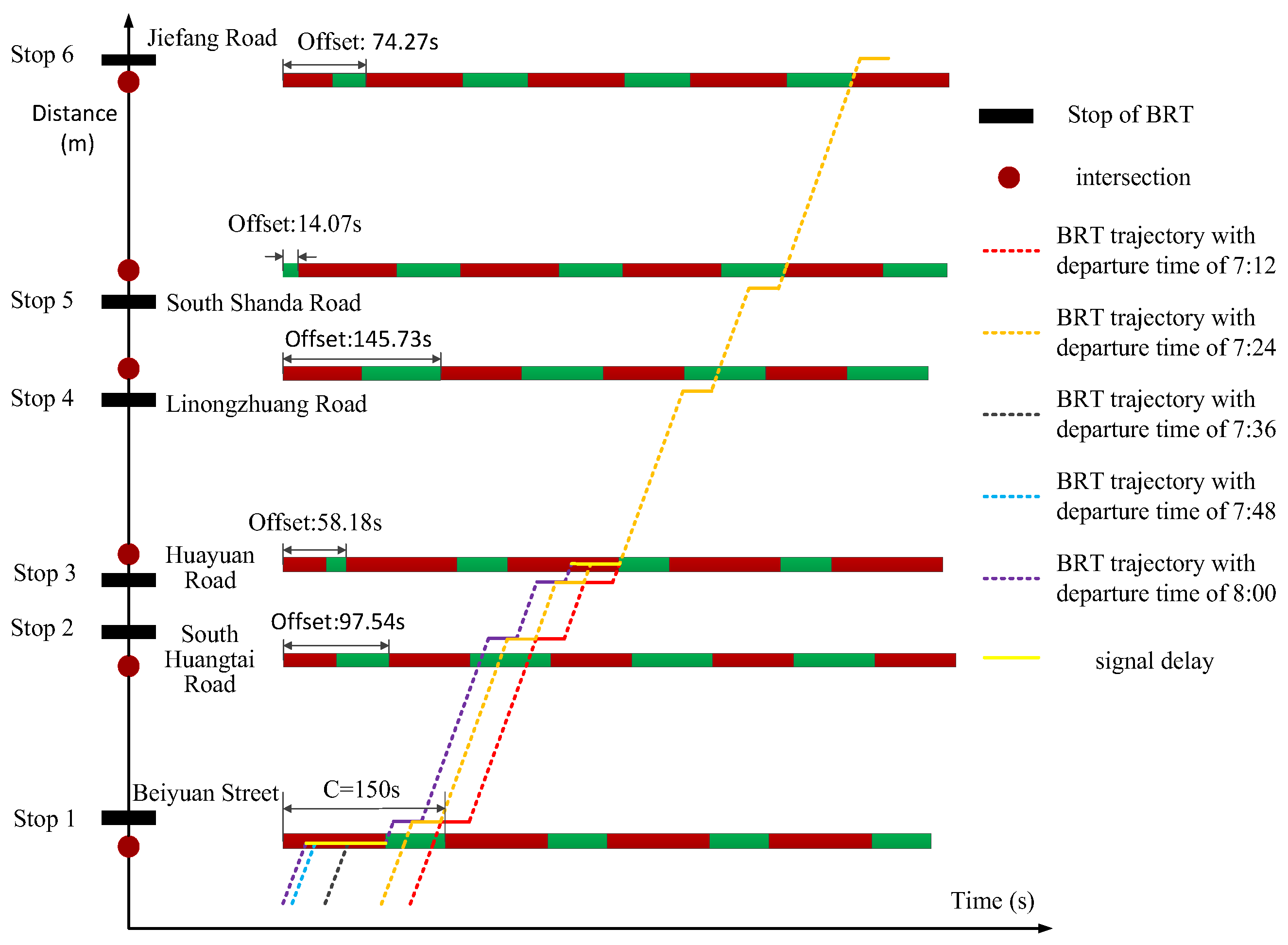
| Schemes | Direction | Offset of intersections (s) | |||||
| Beiyuan Street | Huangtai Road | Huayuan Road | Lilongzhuang Road | South Shanda Road | Jiefang Road | ||
| Proposed scheme | Outbound | 0.00 | 97.54 | 58.18 | 145.73 | 10.82 | 74.27 |
| Inbound | 75.73 | 23.27 | 133.91 | 71.45 | 86.55 | 0.00 | |
| Scheme 1 | Outbound | 0 | 44 | 66 | 78 | 14 | 114 |
| Inbound | 36 | 80 | 102 | 114 | 50 | 0 | |
| Scheme 2 | Outbound | 0 | 44 | 66 | 78 | 14 | 114 |
| Inbound | 36 | 80 | 102 | 114 | 50 | 0 | |
| Scheme 3 | Outbound | 0 | 75.2 | 75.2 | 136.8 | 15.6 | 90.1 |
| Inbound | 59.9 | 135.1 | 135.1 | 46.7 | 75.5 | 0 | |
| Scheme 4 | Outbound | 0 | 44 | 66 | 78 | 14 | 114 |
| Inbound | 36 | 80 | 102 | 114 | 50 | 0 | |
| Scheme 5 | Outbound | 0 | 91.9 | 51.8 | 139.4 | 14.1 | 68.7 |
| Inbound | 81.3 | 23.3 | 133.1 | 70.6 | 95.4 | 0.0 | |
| Scheme 6 | Outbound | 0 | 44 | 66 | 78 | 14 | 114 |
| Inbound | 36 | 80 | 102 | 114 | 50 | 0 | |
| Scheme 7 | Outbound | 0.0 | 91.0 | 50.9 | 139.4 | 6.2 | 67.8 |
| Inbound | 82.2 | 23.3 | 133.1 | 71.6 | 88.5 | 0.0 | |
| Schemes | Entering Time | Direction | Delay of BRT at the Intersections (s) | |||||||
|---|---|---|---|---|---|---|---|---|---|---|
| Beiyuan Street | Huangtai Road | Huayuan Road | Lilongzhuang Road | South Shanda Road | Jiefang Road | Total One-Way Delay | Total Two-Way Delay | |||
| Proposed scheme | 7:12 | Outbound | 0.0 | 0.0 | 0.0 | 0.0 | 0.0 | 0.0 | 0.0 | 0.0 |
| Inbound | 0.0 | 0.0 | 0.0 | 0.0 | 0.0 | 0.0 | 0.0 | |||
| 7:24 | Outbound | 0.0 | 0.0 | 30.0 | 0.0 | 0.0 | 0.0 | 30.0 | 41.8 | |
| Inbound | 0.0 | 0.0 | 0.0 | 11.8 | 0.0 | 0.0 | 11.8 | |||
| 7:36 | Outbound | 15.0 | 0.0 | 45.0 | 0.0 | 0.0 | 0.0 | 60.0 | 101.8 | |
| Inbound | 0.0 | 0.0 | 0.0 | 30.5 | 1.3 | 10.0 | 41.8 | |||
| 7:48 | Outbound | 45.0 | 0.0 | 45.0 | 0.0 | 0.0 | 0.0 | 90.0 | 161.8 | |
| Inbound | 0.0 | 0.0 | 0.0 | 30.5 | 1.3 | 40.0 | 71.8 | |||
| 8:00 | Outbound | 75.0 | 0.0 | 45.0 | 0.0 | 0.0 | 0.0 | 120.0 | 221.8 | |
| Inbound | 0.0 | 0.0 | 0.0 | 30.5 | 1.3 | 70.0 | 101.8 | |||
| Scheme 1 | 7:12 | Outbound | 79.0 | 0.0 | 0.0 | 0.0 | 15.2 | 35.5 | 129.7 | 336.5 |
| Inbound | 39.0 | 67.8 | 49.5 | 14.8 | 35.5 | 0.0 | 206.7 | |||
| 7:24 | Outbound | 0.0 | 46.0 | 17.8 | 19.5 | 40.8 | 35.5 | 159.7 | 396.5 | |
| Inbound | 39.0 | 67.8 | 49.5 | 14.8 | 65.5 | 0.0 | 236.7 | |||
| 7:36 | Outbound | 0.0 | 0.0 | 93.8 | 19.5 | 40.8 | 35.5 | 189.7 | 456.5 | |
| Inbound | 39.0 | 67.8 | 49.5 | 14.8 | 85.5 | 10.0 | 266.7 | |||
| 7:48 | Outbound | 19.0 | 0.0 | 0.0 | 0.0 | 15.2 | 35.5 | 69.7 | 366.5 | |
| Inbound | 39.0 | 67.8 | 49.5 | 14.8 | 85.5 | 40.0 | 296.7 | |||
| 8:00 | Outbound | 49.0 | 0.0 | 0.0 | 0.0 | 15.2 | 35.5 | 99.7 | 426.5 | |
| Inbound | 39.0 | 67.8 | 49.5 | 14.8 | 85.5 | 70.0 | 326.7 | |||
| Scheme 2 | 7:12 | Outbound | 79.0 | 0.0 | 0.0 | 0.0 | 15.2 | 9.5 | 103.7 | 284.4 |
| Inbound | 13.0 | 41.8 | 51.9 | 0.0 | 0.0 | 74.0 | 180.7 | |||
| 7:24 | Outbound | 0.0 | 46.0 | 17.8 | 19.5 | 40.8 | 9.5 | 133.6 | 194.3 | |
| Inbound | 13.0 | 41.8 | 5.9 | 0.0 | 0.0 | 0.0 | 60.7 | |||
| 7:36 | Outbound | 0.0 | 0.0 | 93.8 | 19.5 | 40.8 | 9.5 | 163.6 | 254.3 | |
| Inbound | 13.0 | 41.8 | 35.9 | 0.0 | 0.0 | 0.0 | 90.7 | |||
| 7:48 | Outbound | 19.0 | 0.0 | 0.0 | 0.0 | 15.2 | 9.5 | 43.7 | 164.4 | |
| Inbound | 13.0 | 41.8 | 51.9 | 0.0 | 0.0 | 14.0 | 120.7 | |||
| 8:00 | Outbound | 49 | 0.0 | 0.0 | 0.0 | 15.2 | 9.5 | 73.7 | 224.5 | |
| Inbound | 13.0 | 41.8 | 51.9 | 0.0 | 0.0 | 44.0 | 150.7 | |||
| Scheme 3 | 7:12 | Outbound | 0.0 | 0.0 | 18.7 | 0.0 | 0.0 | 64.8 | 83.5 | 91.5 |
| Inbound | 0.0 | 0.0 | 0.0 | 0.0 | 8.0 | 0.0 | 8.0 | |||
| 7:24 | Outbound | 0.0 | 0.0 | 48.7 | 0.0 | 0.0 | 64.8 | 113.5 | 151.5 | |
| Inbound | 0.0 | 0.0 | 0.0 | 38.0 | 0.0 | 0.0 | 38.0 | |||
| 7:36 | Outbound | 15.0 | 0.0 | 63.7 | 0.0 | 0.0 | 64.8 | 143.5 | 211.5 | |
| Inbound | 0.0 | 0.0 | 0.0 | 58.0 | 0.0 | 10.0 | 68.0 | |||
| 7:48 | Outbound | 45.0 | 0.0 | 63.7 | 0.0 | 0.0 | 64.8 | 173.5 | 271.5 | |
| Inbound | 0.0 | 0.0 | 0.0 | 58.0 | 0.0 | 40.0 | 98 | |||
| 8:00 | Outbound | 75.0 | 0.0 | 63.7 | 0.0 | 0.0 | 64.8 | 203.5 | 331.5 | |
| Inbound | 0.0 | 0.0 | 0.0 | 58.0 | 0.0 | 70.0 | 128 | |||
| Scheme 4 | 7:12 | Outbound | 79.0 | 0.0 | 78.8 | 45.5 | 40.8 | 9.5 | 253.7 | 434.5 |
| Inbound | 39.0 | 41.8 | 25.9 | 0.0 | 0.0 | 74.0 | 180.7 | |||
| 7:24 | Outbound | 0.0 | 46.0 | 0.0 | 37.4 | 40.8 | 9.5 | 133.7 | 344.5 | |
| Inbound | 39.0 | 41.8 | 64.4 | 0.0 | 65.5 | 0.0 | 210.7 | |||
| 7:36 | Outbound | 0.0 | 0.0 | 67.8 | 45.5 | 40.8 | 9.5 | 163.7 | 254.5 | |
| Inbound | 39.0 | 41.8 | 9.9 | 0.0 | 0.0 | 0.0 | 90.7 | |||
| 7:48 | Outbound | 19.0 | 0.0 | 78.8 | 45.5 | 40.8 | 9.5 | 193.7 | 314.5 | |
| Inbound | 39.0 | 41.8 | 25.9 | 0.0 | 0.0 | 14.0 | 120.7 | |||
| 8:00 | Outbound | 49.0 | 0.0 | 78.8 | 45.5 | 40.8 | 9.5 | 223.7 | 374.5 | |
| Inbound | 39.0 | 41.8 | 25.9 | 0.0 | 0.0 | 44.0 | 150.7 | |||
| Scheme 5 | 7:12 | Outbound | 79.0 | 0.0 | 64.6 | 0.0 | 0.0 | 64.8 | 207.5 | 339.5 |
| Inbound | 0.0 | 0.0 | 0.0 | 50.1 | 6.9 | 74.0 | 132.0 | |||
| 7:24 | Outbound | 0.0 | 0.0 | 23.6 | 0.0 | 0.0 | 64.8 | 87.5 | 99.5 | |
| Inbound | 0.0 | 0.0 | 0.0 | 12.0 | 0.0 | 0.0 | 12.0 | |||
| 7:36 | Outbound | 0.0 | 0.0 | 53.6 | 0.0 | 0.0 | 64.8 | 118.4 | 159.5 | |
| Inbound | 0.0 | 0.0 | 0.0 | 41.1 | 0.0 | 0.0 | 41.1 | |||
| 7:48 | Outbound | 19.0 | 0.0 | 64.6 | 0.0 | 0.0 | 64.8 | 148.4 | 219.4 | |
| Inbound | 0.0 | 0.0 | 0.0 | 50.1 | 6.9 | 14.0 | 71 | |||
| 8:00 | Outbound | 49.0 | 0.0 | 64.6 | 0.0 | 0.0 | 64.8 | 178.4 | 279.4 | |
| Inbound | 0.0 | 0.0 | 0.0 | 50.1 | 6.9 | 44.0 | 101.0 | |||
| Scheme 6 | 7:12 | Outbound | 0.0 | 42.0 | 0.0 | 37.4 | 40.8 | 9.5 | 129.7 | 336.5 |
| Inbound | 39.0 | 41.8 | 64.4 | 0.0 | 61.5 | 0.0 | 206.7 | |||
| 7:24 | Outbound | 0.0 | 72.0 | 0.0 | 37.4 | 40.8 | 9.5 | 159.7 | 246.5 | |
| Inbound | 39.0 | 41.8 | 0.0 | 0.0 | 5.9 | 0.0 | 86.7 | |||
| 7:36 | Outbound | 15.0 | 0.0 | 78.8 | 45.5 | 40.8 | 9.5 | 189.7 | 306.5 | |
| Inbound | 39.0 | 41.8 | 25.9 | 0.0 | 0.0 | 10.0 | 116.7 | |||
| 7:48 | Outbound | 45.0 | 0.0 | 78.8 | 45.5 | 40.8 | 9.5 | 219.7 | 366.5 | |
| Inbound | 39.0 | 41.8 | 25.9 | 0.0 | 0.0 | 40.0 | 146.7 | |||
| 8:00 | Outbound | 75.0 | 0.0 | 78.8 | 45.5 | 40.8 | 9.5 | 249.7 | 426.5 | |
| Inbound | 39.0 | 41.8 | 25.9 | 0.0 | 0.0 | 70.0 | 176.7 | |||
| Scheme 7 | 7:12 | Outbound | 0.0 | 0.0 | 18.7 | 0.0 | 0.0 | 64.8 | 83.5 | 91.5 |
| Inbound | 0.0 | 0.0 | 0.0 | 8.0 | 0.0 | 0.0 | 8.0 | |||
| 7:24 | Outbound | 0.0 | 0.0 | 48.7 | 0.0 | 0.0 | 64.8 | 113.5 | 151.5 | |
| Inbound | 0.0 | 0.0 | 0.0 | 38.0 | 0.0 | 0.0 | 38.0 | |||
| 7:36 | Outbound | 15.0 | 0.0 | 63.7 | 0.0 | 0.0 | 64.8 | 143.5 | 211.5 | |
| Inbound | 0.0 | 0.0 | 0.0 | 58.0 | 0.0 | 10.0 | 68.0 | |||
| 7:48 | Outbound | 45.0 | 0.0 | 63.7 | 0.0 | 0.0 | 64.8 | 173.5 | 271.5 | |
| Inbound | 0.0 | 0.0 | 0.0 | 58.0 | 0.0 | 40.0 | 98.0 | |||
| 8:00 | Outbound | 75.0 | 0.0 | 63.7 | 0.0 | 0.0 | 64.8 | 203.5 | 331.5 | |
| Inbound | 0.0 | 0.0 | 0.0 | 58.0 | 0.0 | 70.0 | 128 | |||
Disclaimer/Publisher’s Note: The statements, opinions and data contained in all publications are solely those of the individual author(s) and contributor(s) and not of MDPI and/or the editor(s). MDPI and/or the editor(s) disclaim responsibility for any injury to people or property resulting from any ideas, methods, instructions or products referred to in the content. |
© 2023 by the authors. Licensee MDPI, Basel, Switzerland. This article is an open access article distributed under the terms and conditions of the Creative Commons Attribution (CC BY) license (https://creativecommons.org/licenses/by/4.0/).
Share and Cite
Wu, W.; Luo, X.; Shi, B. Offset Optimization Model for Signalized Intersections Considering the Optimal Location Planning of Bus Stops. Systems 2023, 11, 366. https://doi.org/10.3390/systems11070366
Wu W, Luo X, Shi B. Offset Optimization Model for Signalized Intersections Considering the Optimal Location Planning of Bus Stops. Systems. 2023; 11(7):366. https://doi.org/10.3390/systems11070366
Chicago/Turabian StyleWu, Wei, Xiaoyu Luo, and Baiying Shi. 2023. "Offset Optimization Model for Signalized Intersections Considering the Optimal Location Planning of Bus Stops" Systems 11, no. 7: 366. https://doi.org/10.3390/systems11070366
APA StyleWu, W., Luo, X., & Shi, B. (2023). Offset Optimization Model for Signalized Intersections Considering the Optimal Location Planning of Bus Stops. Systems, 11(7), 366. https://doi.org/10.3390/systems11070366