Agricultural Green Ecological Efficiency Evaluation Using BP Neural Network–DEA Model

Abstract

The evaluation of agricultural green ecological efficiency can reflect the capacity of agriculture for sustainable development and reduce the endogenous pollution caused by agricultural waste in order to alleviate the weakening of agricultural ecosystems. Taking the agricultural green economy as the research object, an evaluation index system based on the theories of green economic efficiency and economic growth for agricultural green ecological efficiency was constructed, and the impact mechanisms of specific indicators on agricultural green ecological efficiency were empirically explored. In addition, based on the data envelopment analysis (DEA) model, the overall agricultural green ecological efficiency of China from 2002 to 2021 was evaluated and the efficiency characteristics were analyzed from multiple perspectives. Then, the indicators of policy, finance, communication, society and other aspects were added in order to construct a comprehensive evaluation model of agricultural green ecological efficiency using a combination of DEA and a BP neural network, and the feasibility of the model was verified. The results indicate that the agricultural green ecological efficiency increased from 0.7340 in 2002 to 0.8205 in 2021, an increase of 11.78%. Additionally, the technological efficiency of China’s agricultural green ecological system did not show a very obvious trend of divergence. The results of the BP neural network were consistent with those obtained using DEA, and the overall evolution trend of the calculated BP neural network and DEA were mutually verified and integrated. The effectiveness and accuracy of the BP neural network was verified via a comparison with DEA.

1. Introduction

The great economic development and rapid industrialization of the past thirty years in China have brought about a series of economic and social challenges. Industry is an important force driving rapid economic growth and plays a critical role in the agricultural economy. The correct handling of the relationship between the environment and development, and guiding the transformation of traditional development methods towards green development approaches, is a prerequisite for the development of regional innovation ecosystems. Therefore, it is feasible to incorporate environmental factors, such as the environmental output, into the technological innovation framework in order to measure and analyze the efficiency of green technology innovation in rural industries, achieve resource allocation and technological innovation, and better coordinate sustainable economic and environmental development. However, the prerequisites for green technology innovation in enterprises include developing methods to scientifically and objectively evaluate the effectiveness of green technology innovation in rural industrial enterprises in China, and analyze the distribution characteristics and changing trends observed in the green technology innovation performance of industrial enterprises in rural areas in order to more effectively improve the efficiency and technological level of green innovation in enterprises.

To this end, Liu [1] used panel-corrected standard error regression to study the impact of renewable energy use on GDP and local agricultural income. The study found that the use of renewable energy in rural areas had a significant positive impact on the income growth of rural households. It was not only an important measure to solve the energy crisis and global warming, but also an important force to promote industrial restructuring and rural development. Due to the increasingly serious resource and environmental issues worldwide, the rational use of agricultural inputs to promote green development in rural areas has become increasingly important. Wang et al. [2] found that the intensity of agricultural investment was positively correlated with the planting convenience and urbanization rate, but negatively correlated with planting structure. Therefore, the planting structure should be optimized and circular agriculture should be developed according to local conditions.

In terms of research methods, an indicator system is usually used to construct an ecological efficiency evaluation system to measure the coordination between society, the economy and the environment. For example, Orea and Wall [3] used the input/output ratio and economic efficiency/pollution ratio to evaluate the ecological efficiency of the UK’s aluminum and steel industries. Zhang et al. [4] used the ecological footprint method to measure the ecological environment of the belt and road region. In addition, natural factors such as land, water, raw materials, energy and carbon emissions can also be selected as evaluation indicators for ecological efficiency [5].

The current methods used to calculate ecological efficiency are mainly the ecological footprint method, energy analysis method and data envelopment analysis (DEA), of which the most common method is data envelopment analysis. However, DEA cannot effectively rank the data of decision-making units, which will ultimately have a negative impact on the accuracy and comprehensiveness of the estimation results. Therefore, a BP neural network–DEA model, designed to comprehensively evaluate the ecological efficiency of the agricultural green industry, was constructed in this study. In addition, the evaluation indicators of industrial ecological efficiency were also based on a macro-level regional ecological efficiency measurement. In fact, when evaluating the ecological efficiency of industry comprehensively, not only macro aspects should be fully considered, but also the reality of industrial ecological efficiency and the industrial production situation in order to more intuitively reflect the trend of industrial change. Thus, this article selected indicators that are in line with the actual situation in rural areas and improves the ecological evaluation index system of the agricultural green industry. The innovations of this paper are as follows: (1) an agricultural green ecological system, including agricultural carbon emissions and green GDP as part of the ecological environment factors, was proposed. (2) A BP neural network model, combined with a DEA model, was used to further evaluate the agricultural green ecological efficiency.

This article mainly explored the application of optimization methods that can be used to evaluate the agricultural green ecological efficiency. First, based on the construction of an evaluation index system for agricultural green ecological efficiency, the impacts of specific indicators on agricultural green ecological efficiency were explored. Additionally, the green ecological efficiency of China’s agricultural industry from 2002 to 2021 was calculated and analyzed using a DEA model. Then, the evaluation results of the DEA efficiency were used as the expected output of the evaluation results when establishing the BP neural network model. After selecting a more comprehensive indicator system, a BP neural network model was used to further evaluate the agricultural green ecological efficiency, and the differences between the two evaluation methods were analyzed. Finally, policy recommendations are provided based on the research conclusions. The article’s structure is as follows: Section 2 contains the materials and methods. Section 3 introduces the construction of the agricultural green ecological efficiency model. Section 4 describes the construction of the evaluation index system for agricultural green ecological efficiency and the source of the research data. Section 5 is an empirical study of the indicator system used for agricultural green ecological efficiency. Section 6 is the measurement of agricultural green ecological efficiency based on the DEA model. Section 7 discusses the evaluation results of agricultural green ecological efficiency based on the BP neural network model compared with DEA in order to verify the feasibility of the BP neural network model. Section 8 contains the conclusion and recommendations, as well as directions for future research.

2. Materials and Methods

2.1. Theoretical Analysis of Green Economic Efficiency

Efficiency has different definitions in different fields. It is precisely because of the diversification and difference between fields that there are large differences and disputes regarding the final definition of efficiency [6]. Efficiency from an economic perspective refers to the allocation efficiency of production factor resources in the market and economy [7,8].

Economics is a discipline that studies how to more effectively allocate scarce resources in society in order to achieve maximum utility [9]. To a certain extent, “efficiency”, under the existing scientific, technological and production conditions, means maximizing the use of scarce resources as much as possible to obtain more output and profits [10].

In the modern economic growth theory, the study of economic efficiency mainly uses the aggregate production function. Some measures of economic efficiency are directly derived from relevant economic growth theories such as the production function method. Among them, one of the more classic and commonly used economic growth models is the Solow model [11]. Based on the Solow model, Solow pioneered the analysis and research of economic growth accounting, measuring the contribution of different production factors in the process of economic growth.

Since the middle of the last century, with the rapid economic growth, more and more problems have become increasingly prominent. Among them, environmental issues have always plagued the government’s economic decision making and the normal life of citizens [12]. However, traditional economic efficiency analysis does not take environmental pollution into account, resulting in a significantly higher efficiency value. At the same time, ignoring environmental pollution and conducting research on regional economic efficiency may lead to conclusions that deviate from reality and may even be completely different. Moreover, some regions may have a lower economic efficiency than other regions, but their environmental control is better [13]. This kind of regional economic efficiency evaluation index system that does not consider ecological costs will cause some local governments to overemphasize an increase in GDP, while ignoring the protection of the ecological environment. At the same time, they cannot scientifically and reasonably evaluate the actual economic development level of the region. For this reason, many scholars have begun to consider environmental pollution when calculating economic efficiency, and have proposed the concept of green economic efficiency [14,15]. Some researchers believe that green economy efficiency is an indicator that can determine the total inflow of resources and the cost of environmental pollution, and can measure and evaluate the economic performance of a country or region. To a certain extent, it mainly includes two aspects: (1) green economy efficiency is used as an indicator to evaluate the measured regional economic performance; it is the measurement and calculation of the utilization efficiency of factor inputs in economic development, and it also refers to the region’s gains through unit factor inputs in relation to the expected outputs. (2) Green economic efficiency scientifically and logically considers factor inputs and the undesired outputs, and incorporates the use of production factors and environmental pollution costs into the process of economic development activities. The calculated efficiency refers to the original economic efficiency and the “green” economic efficiency after the addition of factor inputs and environmental pollution costs to the model. Therefore, the green economic efficiency is a comprehensive economic efficiency that not only considers the input of factors, but also accommodates the cost of environmental pollution; the larger the value of green economic efficiency, the higher the overall quality of economic development in the region.

2.2. Economic Growth Theory

This theory mainly discusses the role of various production factors in the process of economic growth and how the combination of production factors can better promote economic growth [16]. The earliest research on the issue of economic growth was Adam Smith’s “Theory of the Rich”, which is also the origin of the classical economic growth theory. It mainly elaborates on the two core issues of the source and accumulation of wealth [17,18].

Based on the questioning of the Harold–Domar model “the capitalist market cannot achieve sustained economic growth”, the neoclassical economic theory represented by Solow and Swan was established. The expression of the production function is as follows:

$$\frac{\Delta Y}{Y}=\frac{\Delta T}{T}+\alpha \frac{\Delta M}{M}+\beta \frac{\Delta N}{N}$$

(1)

where $\frac{\Delta Y}{Y}$, $\frac{\Delta M}{M}$ and $\frac{\Delta N}{N}$ are the output growth rates, capital growth rates, and labor growth rates, respectively; $\alpha$ and $\beta$ are the capital and labor shares in output, respectively; and $\frac{\Delta T}{T}$ is the technological progress growth rate.

2.3. Dynamic BP Neural Network

2.3.1. The Structure of Biological Neurons

Nerve cells are the basic unit of the nervous system, called biological neurons, or neurons for short [19,20]. Neurons are mainly composed of three parts, a cell body, axon and dendrites, as shown in Figure 1.

2.3.2. The Structure of Artificial Neural Networks

An artificial neural network is composed of many processors, which are called artificial neurons [21]. Through an interface widely used to simulate the structure and function of the brain nervous system, neural networks can be regarded as using artificial neurons as nodes. They use a directed graph connected by a directed weighted arc. In this directed graph, the artificial neuron simulates a biological neuron, and the directed arc simulates the “axon–synapse–dendrite” connection [22,23]. The weight of the directed arc indicates the strength of the interaction between the two artificial neurons connected to each other. 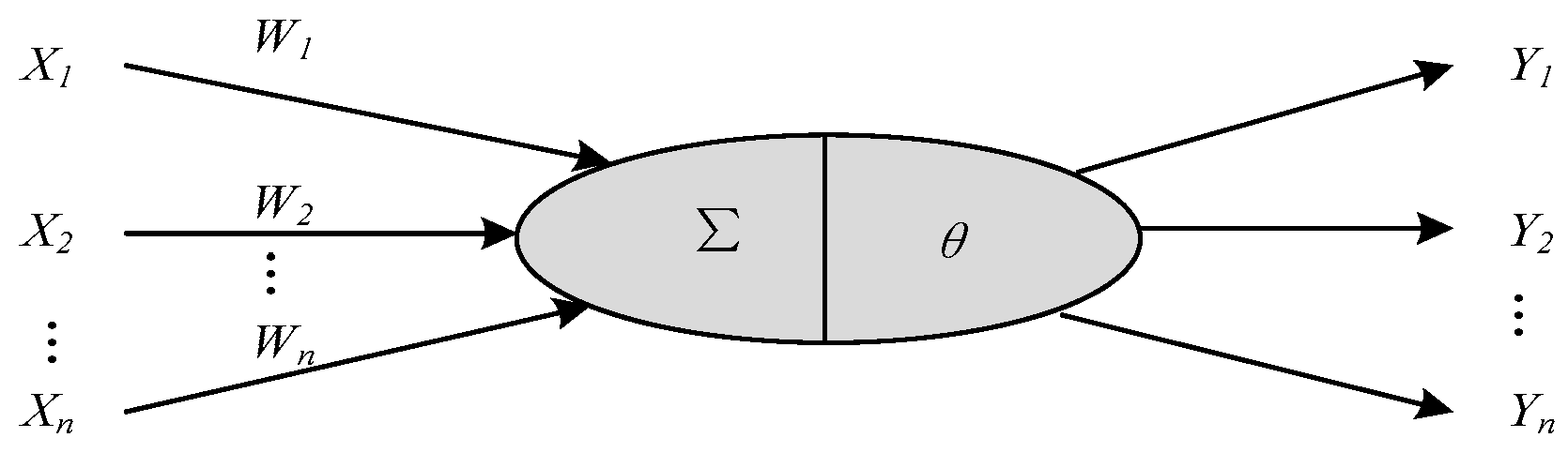The model of each artificial neuron is shown in Figure 2. Using circles to represent the cell body of a neuron, $X_i\left(i=1,2,\cdots ,n\right)$ represents the external input of the neuron, $W_i$ represents the branch strength of the neuron and each cell input, θ represents the neuron boundary and Y represents the neuron output.

In a typical artificial neural network, there are different ways to connect a single neuron, and different connection methods form different network connection modes. Common connection modes includinge the forward network are different from the feedback network throug the input stage to the output stage, and some output data of the output stage are sent to the input layer neuron as network input data [24]. In addition to images, the first two networks also receive the same information from neurons in the previous layer, and neurons in the same layer in the network can also interact with each other and report to the connected network [25].

2.3.3. BP Neural Network and Its Network Structure

The BP (Back Propagation) neural network algorithm, proposed in 1985, realizes Minsky’s multi-level network vision [26,27]. The artificial neurons that make up the multilayer network can be continuously pushed so that the artificial neural network converts the input into the desired output. If the BP neural network algorithm can be regarded as changes and weights, then the connections between neural networks in the network can be regarded as parameter changes. In addition, when the BP neural network algorithm adjusts the weights, the connection of a single fake neuron is based on the difference between the actual network output and the expected output, and this difference will be reversed individually. From the perspective of the combined weight of each type of neuron, the BP neural network algorithm has become the most widely used and most important learning algorithm in neural network training.

The BP neural network topology is a multi-level forwarding network, composed of input-level nodes and output-level nodes, with at least one hidden layer node [28]. In the BP neural network, neurons in the same layer are not connected, and neurons in adjacent layers are connected by weight. When inputting information into the BP neural network, the data are transmitted from the input-level node to the hidden first-level node (artificial neuron), and then the information is transmitted to the next hidden part. The information is transferred one layer at a time, and this continues until it is finally transferred to the output level for output. At the same time, the activation function of each level must be different, and the sigmoid function is usually used. The most basic neural network BP is a power network with three nodes: input layer, hidden layer and output layer. The structure is shown in Figure 3.

2.4. DEA Model

The development of our DEA model for agricultural green ecological efficiency started with the traditional DEA model. DEA can be divided into a fixed performance CCR model and a BBC model with a degraded BCC (TE) technical performance. This model has been reduced to pure technology (PTE) and scale performance (SE) in the performance CCR model:

$$TE=PTE\times SE$$

(2)

It is helpful to judge the degree to which the efficiency of each DMU agricultural green ecological system is affected by pure technical factors and scale factors. BCC is now relatively mature. According to different opinions, there are two types of DEA: input-oriented and conventional. The former has the problem of minimizing the input below a given output, and the latter has the problem of maximizing the output below the input. Given that the input volume is easier to control than the output volume and conforms to the concept of intensive economy, this article chose a BBC model that focuses on input:

$${\displaystyle \sum _{i=1}^I}{\lambda }_i{P}_{a,i}\le {\phi }_i{P}_{a,i},a=1,2,\cdots ,A$$

(3)

$${\displaystyle \sum _{i=1}^I}{\lambda }_i{Q}_{b,i}\le {\phi }_i{Q}_{b,i},b=1,2,\cdots ,B$$

(4)

$${\displaystyle \sum _{i=1}^I}{\lambda }_i=1,{\lambda }_i\ge 0,i=1,2,\cdots ,I$$

(5)

In these formulas, a and b represent the input and output variables, respectively; $P_{a,i}$ is the a-th input of the i-th DMU; $Q_{b,i}$ is the b-th output of the i-th DMU; and ${\lambda }_i$ is the a-th input and the b-th output. The weighting coefficient ${\phi }_i$ is the relative efficiency of the i-th DMU, which is between 0 and 1. Then, the principal components are substituted into the first-stage DEA model, and the first-stage DEA is realized using special software.

The principal component mathematical model is as follows:

$$F_1=u_{11}Z{X}_1+u_{12}Z{X}_2+\cdots +u_{1j}Z{X}_j$$

(6)

$$F_2=u_{21}Z{X}_1+u_{22}Z{X}_2+\cdots +u_{2j}Z{X}_j$$

(7)

$$F_i=u_{i1}Z{X}_1+u_{i2}Z{X}_2+\cdots +u_{ij}Z{X}_j$$

(8)

Among them, $F_i$ is the i-th principal component, $Z{X}_j$ is the original index after the normalization of the j-th term, $u_{ij}$ is the principal component expression coefficient, $u_{ij}=\frac{a_{ij}}{\sqrt{{\lambda }_j}}, A={\left(a_{ij}\right)}_{pxp}$ is the factor loading matrix, and $\lambda$ is the eigenvector.

The accounting method and process used for agricultural green GDP are given below.

The calculation formula for agricultural green GDP is as follows:

Agricultural green GDP = Agricultural conventional GDP + Agricultural ecological GDP

(9)

The expression is as follows:

$${GDP}_g={GDP}_t+{GDP}_e$$

(10)

The conventional agricultural GDP is the output value minus the production cost (i.e., the intermediate consumption), and the agricultural ecological environmental cost mainly refers to the loss of environmental resource value and the loss of ecological value caused by the reduction in the agricultural resource area. It is expressed as follows:

$${GDP}_g={GDP}_t+{GDP}_e=V_p-C_p+V_{es}-C_e$$

(11)

In the formula, $V_p$ is the agricultural output value, $C_p$ is the agricultural production cost (intermediate consumption), $V_{es}$ is the agricultural ecosystem service value and $C_e$ is the agricultural ecological environmental cost. Among them, the agricultural output value and agricultural intermediate consumption refer to the relevant yearbook statistics. The specific steps for calculating the value of the agro-ecological service $V_{es}$ are as follows:

$$E_a=\frac{1}{7}{\displaystyle \sum _{i=1}^n}\frac{m_i{q}_i{p}_i}{M}(i=1,2,\cdots ,n)$$

(12)

where $E_a$ represents the value of the food production function per unit area of farmland, i is the type of food crop, $m_i$ is the sown area of the i-th food crop in that year, $p_i$ is the national average price of the i-th food crop in that year, $q_i$ is the i-th food crop yield per unit area in that year and M is the sum of the sown area of n grain crops.

$$E_{ij}=e_{ij}{E}_a(i=1,2,\cdots ,9;j=1,2,3,4)$$

(13)

where $E_{ij}$ represents the unit price of the i-th ecological service provided by the j-th agricultural resource per unit area and $e_{ij}$ is the i-th ecological service value equivalent factor of the j-th agricultural resource.

$$V={\displaystyle \sum _{i=1}^9}{\displaystyle \sum _{j=1}^4}{A}_j{E}_{ij}(i=1,2,\cdots ,9;j=1,2,3,4)$$

(14)

In the formula, $V$ represents the total value of ecological services of the regional agricultural system and $A_j$ represents the area of type j agricultural resources.

3. Model Construction

3.1. Literature Review of Agricultural Ecological Efficiency Evaluation Method

Agricultural ecological efficiency can be evaluated by the ratio of economic value generated by related goods and services to the effects of the environmental impact generated during the production processes [29,30]. The measurement methods used for agricultural ecological efficiency mainly include the ratio method, life cycle method, ecological footprint method, energy method and data envelopment analysis method [31,32]. The ratio method reflects the impact of economic development on the environment to some extent, but it only considers the output aspect without the input aspect, making it difficult to distinguish between different environmental impacts. The life cycle assessment method has drawbacks such as difficulties in boundary determination, complex data selection and strong subjectivity, which greatly affect its credibility. It also has the problem of weak regional comparability. The ecological footprint analysis method has strong applicability and comparability, but has shortcomings such as single evaluation indicators, and it cannot fully reflect ecological functions [33]. The energy analysis method incorporates resources, economic value and the ecosystem into the accounting system at the same time, but it has several shortcomings, such as inaccurate calculations due to time constraints, regional differences in energy conversion rates and relatively simple indicators.

3.2. Advantages and Disadvantages of DEA

Data envelopment analysis is a systematic analysis method based on linear programming theory that was proposed by Charnes et al. [34] in order to evaluate the relative efficiency of decision-making units (DMUs) using multiple input and output indicators and similar attributes. They proposed the first DEA model and CCR model assuming that returns to scale are constant [35]. Agriculture has a huge and complex system organization, and its internal resources can only be fully utilized after organic integration and transformation. There is a reasonable input and output indicator system for research in the field of agriculture. To evaluate such a system, data envelopment analysis is a very suitable method.

Data envelopment analysis has become a research hotspot since it was first proposed, and various improved models have emerged. In 1984, Banker et al. [36] broke the constant limit of returns to scale of the CCR model and established a BCC model with variable returns to scale. Subsequently, Charnes et al. [37]) proposed the CCGSS model to address the unreasonable assumption that the production possibility set is convex under certain conditions. Then, Charnes et al. [38] proposed a preference-based CCWH model.

The vast majority of problems in real life exhibit significant nonlinearity [39] and as a complex system organization, the input–output efficiency of agriculture is not a simple linear relationship. The DEA model can quantitatively and objectively evaluate the effectiveness of decision units, and can also provide improved methods based on relaxed variable results for non-DEA effective decision units [40]. However, the DEA model is generated based on linear programming theory, which may not be suitable for studying problems in real life. At the same time, the DEA model also has certain limitations on the number of indicators because more indicators can affect the feasible solutions and evaluation results.

The BP neural network method can effectively help overcome the aforementioned problems of DEA models [41]. First, BP neural networks have no limit on the number of indicators. Second, BP neural networks simulate the non-linear thinking mode of the human brain to process the received information, which can better fit real-world problems. However, BP neural networks require a certain number of original sample datasets for processing and learning, and process new samples based on the learned knowledge. For the evaluation of agricultural ecological efficiency, specifying a learning sample will lose its quantification and objectivity, so the DEA method is needed to provide objective learning samples for the BP neural network.

3.3. Model Establishment

Firstly, a DEA model was used to conduct the first efficiency evaluation on all decision-making units, and then the results of the first efficiency evaluation were used as the expected output of the second BP neural network evaluation. At the same time, more comprehensive evaluation indicators were introduced to train and teach the BP neural network, and then a second efficiency evaluation was conducted. A comprehensive evaluation of agricultural ecological efficiency was conducted using the evaluation results of the DEA model and BP neural network, which not only retained the advantages of the two methods, but also compensated for their respective shortcomings.

4. Evaluation Index System of Agricultural Green Ecological System

4.1. Establishment of Evaluation Index System

The prerequisite for the accurate evaluation of agricultural ecological efficiency is the construction of reasonable input and output indicators in order to obtain relatively accurate and objective evaluation results. The calculation of agricultural ecological efficiency refers to the ecological economic efficiency of agriculture, which includes both economic and ecological environmental factors, comprehensively reflecting the situation of economic development and environmental protection [42,43]. Therefore, this article mainly selected indicators based on economic development and environmental protection factors. The input and expected output indicators mainly reflected the dimension of agricultural economic growth, while the non-expected output mainly reflected the dimension of agricultural ecological environment protection [44,45]. The resource conservation dimension can be reflected in the input, expected output, and non-expected output indicators [46]. In the process of constructing an evaluation index system for the agricultural ecological efficiency, the input–output indicators and their characteristic variables of agricultural ecological efficiency in China were finally determined.

Since the evaluation of the agricultural green economy in the context of smart cities is based on the idea of sustainable development, it is well known that sustainable development comprises three elements: ecology, economy, and society. Based on the theory of regional ecological systems, the Analytic Hierarchy Process was used to build a green agriculture index in China. The index system of the ecological system is shown in

Table 1. DEA evaluation index system of agricultural green ecological system.

Target Layer	Criterion Layer	Index Layer
		Input	Output
Agricultural Green Ecological System	Agricultural economic and social subsystem F1	Total sown area of crops Number of employed persons in rural areas Total power of agricultural machinery	Per capita net income of agricultural households Urbanization rate
	Agricultural scientific and technological innovation subsystem F2	Financial expenditure for agriculture Forestry and water affairs	Number of agricultural patents Agricultural scientific and technological achievements
	Agricultural green development subsystem F3	Amount of agricultural fertilizer Agricultural electricity consumption Agricultural energy input Energy promotion manager	Forest coverage Green GDP Agricultural carbon emissions

.

In the agricultural economic and social subsystem, labor, land and technology are the most important input elements in the agricultural production process. The output variables included economic and social aspects. Then, the urbanization rate was selected as the proxy indicator of agricultural social development to represent the development process of society in rural areas.

In the agricultural scientific and technological innovation subsystem, the input variables were reflected in the capital and manpower of the sector, in view of the large differences in the statistical caliber of some funds and employees in agricultural science and technology. In terms of agricultural scientific and technological innovation output, the number of agricultural patents and agricultural scientific and technological achievements were selected to characterize the scientific and technological production capacity. This article believes that the inaccessibility of data is one of the reasons why the current research on the performance evaluation of the agricultural ecological system is restricted.

In the agricultural green development subsystem, four indicators (agricultural fertilizer application, agricultural electricity consumption, agricultural energy input and energy extension management personnel) were selected as green ecological input indicators, which more comprehensively characterize the resource consumption in the agricultural production process and management investment. Three indicators of forest coverage (total gas production from agricultural biogas digesters and green GDP) were selected as the expected outputs in order to measure the protection capacity and economic benefits to the ecological environment. In contrast to previous studies, this article introduced agricultural green GDP as a green output indicator because plantations, animal husbandry, forestry and fishery benefit from ecosystem services and provide ecosystem services, and the impact of these areas on ecosystem services may be beneficial or unfavorable. To a certain extent, agricultural green GDP can measure the ecological functions of agricultural activities. However, previous studies only used black-box input–output methods without considering this process. Agricultural carbon emissions was selected as the undesired output. At this stage, agricultural carbon emissions are the inevitable pollution produced by the agricultural production process, and it is very necessary to include them in the evaluation system. As China currently does not pay enough attention to agricultural pollution and has not adopted specific policies, systems and regulatory measures to control the pollution of the ecological environment caused by agricultural production activities, this article did not consider the inclusion of industrial-based “pollution control completed investment” and other indicators related to the strength of environmental regulations.

The agricultural green ecological process is not only affected by the internal composition and relationships, but also by external environmental factors. According to whether it directly participates in the agricultural green ecological process, these environment factors can be divided into internal and external factors. Internal influencing factors are related to infrastructure and local labor quality. Infrastructure construction provides the necessary material and information support for green innovation, and represents a systematic hardware support function. Drawing on the research of relevant scholars, infrastructure construction was expressed as the proportion of total post and telecommunications as a proportion of GDP. The quality of regional agricultural laborers is another important factor for transforming green innovation into productivity. The quality of agricultural laborers was expressed by the average number of years of education of farmers.

External factors include natural disasters, the economic development level, the financial environment, and government intervention, because agriculture is different from other industries. The production site itself, as a component of the ecosystem, is greatly affected by natural disasters. The disaster rate was used to express the extent of regional disasters and the per capita GDP indicates the level of economic development. A loose financial environment helps farmers, the government and scientific research institutions to raise funds and capital flow; the regional financial environment was expressed in terms of the loan-to-deposit ratio. The government has a strong leading role in the process of agricultural green ecological development, and science and technology innovation. The proportion of expenditure in agriculture out of the total government expenditure indicates the government’s support and intervention in science and technology. The second stage was realized using Frontier 4.0 software. The environmental factor variables of the agricultural green ecological system are shown in

Table 2. Environmental variables of agricultural green ecological systems.

Environment Variable	Proxy Index
infrastructure	post and telecommunications business volume/GDP (PT)
qualities of workers	average years of education (AE)
natural disaster	disaster rate (DR)
financial environment	loan-to-deposit ratio (LR)
economic level	GDP per capita (GDPC)
government technology support	technology expenditure/total expenditure (TE)

.

4.2. Data Sources

Considering the rationality, scientific basis and operability of indicator selection, as well as the availability of indicator data in the China Statistical Yearbook, the research scope was determined as the measurement of China’s agricultural ecological efficiency from 2001 to 2021. The sample data were all from the 2002 to 2021 China Statistical Yearbook, China Agricultural Yearbook, China Rural Statistical Yearbook, and local statistical yearbooks of various provinces, municipalities and autonomous regions.

5. Analysis of Influencing Factors on Agricultural Green Ecological Efficiency

5.1. Efficiency Analysis of Agricultural Green Ecological System

In order to eliminate the influence of environmental factors and random errors in measuring the effectiveness of the agricultural green ecological system, the loose input of each variable obtained by DEA was traditionally regarded as the dependent variable. The environmental factors were selected as independent variables, and frontier production function regression analysis was performed. The regression results are shown in

Table 3. Value of ${\delta }^2$ and $\lambda$ in agricultural green ecological system.

Independent Variable	F1	F2	F3
${\delta }^2$	68.957	305.258	451.854
$\lambda$	1	1	1

.

Table 3 shows that the one-sided error likelihood ratio statistics were all greater than the chi-squared distribution test’s standard value, and were significant at the 1% test level, indicating that the setting was reasonable. The γ value was approximately 1 and reached the 1% significance level, indicating the main source of error was the technical inefficiency item; therefore, it was appropriate to use the SFA regression model. Input slack refers to the part of the input that can be corrected by improving management methods or adjusting the production scale. From the discussion of the three-stage DEA model, it can be seen that if the SFA regression coefficient is positive, it means that the increase in the environmental variable is conducive to the input slack. On the contrary, when the regression coefficient is negative, it is conducive to the improvement of the efficiency of the agricultural green ecological system.

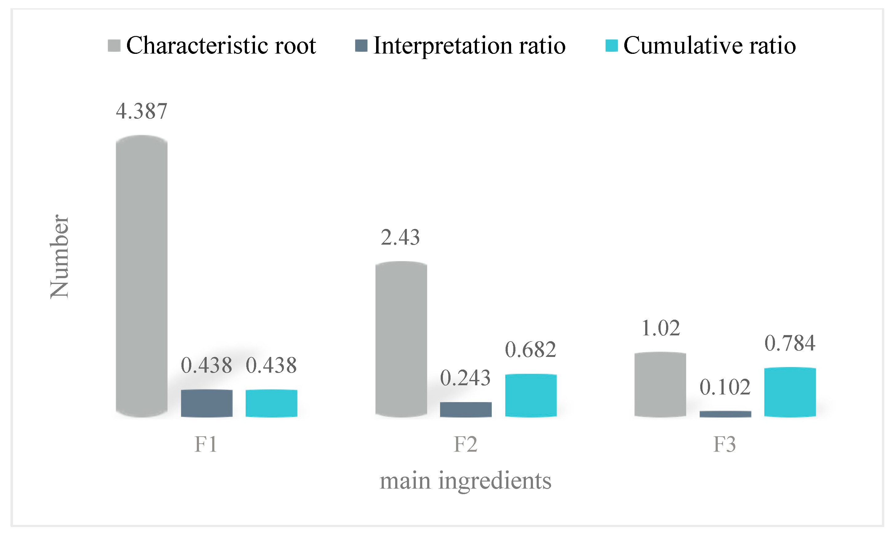
The input variables here are the three input principal components that have been transformed, and the principal component analysis results are shown in Figure 4. In Figure 4, F1, F2, and F3 are the three principal component variables that replaced the ten original input variables. In F1, the total sown area of crops, the number of agricultural employees, the total power of agricultural machinery, and the application amount of agricultural fertilizers were the four index load coefficients, which can be summarized as basic agricultural inputs. In F2, the agricultural electricity consumption load factor was relatively large, which was called investment in environmental protection research. In F3, the load factor of fiscal expenditure for agriculture, forestry and water affairs was large, which was called government financial support.

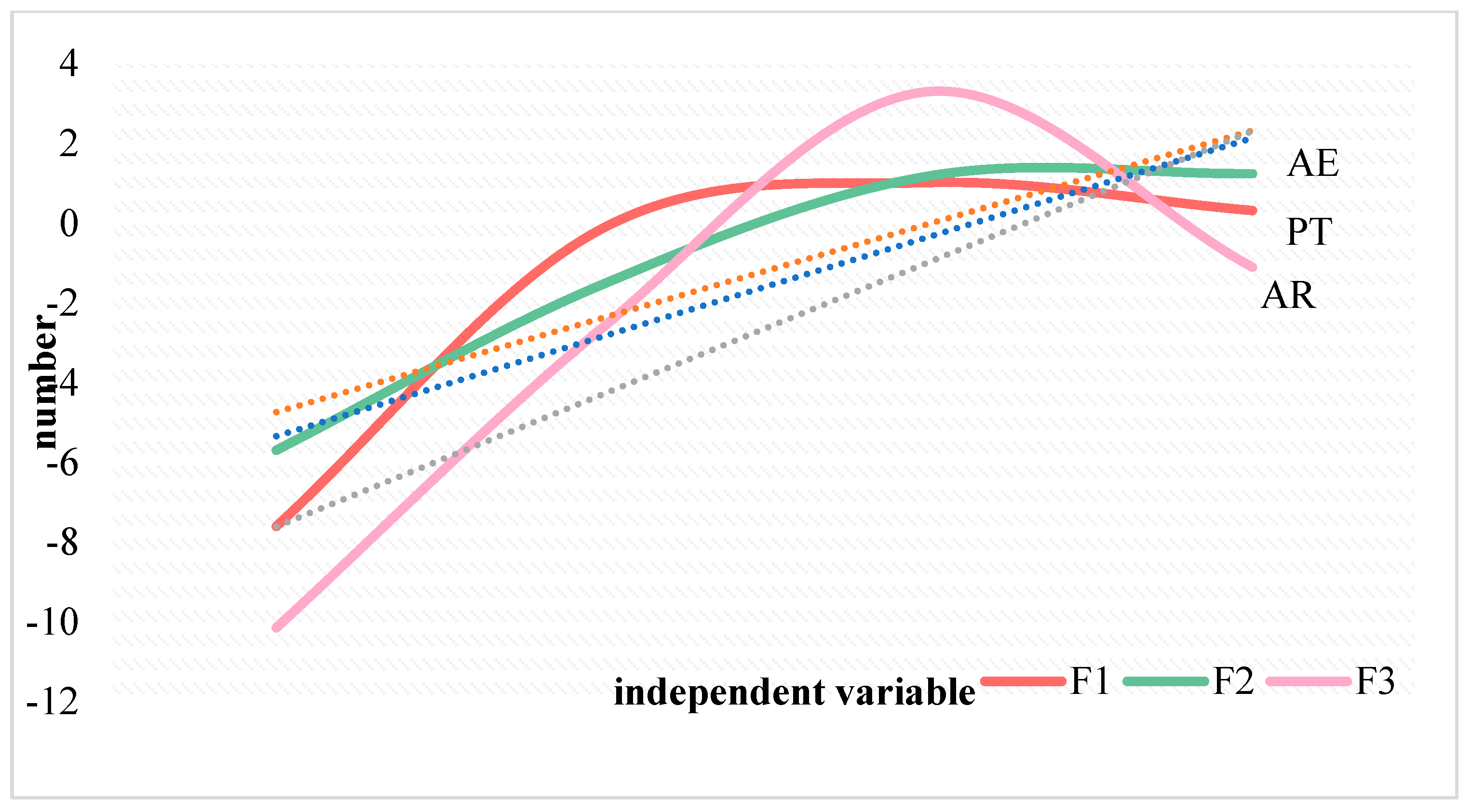
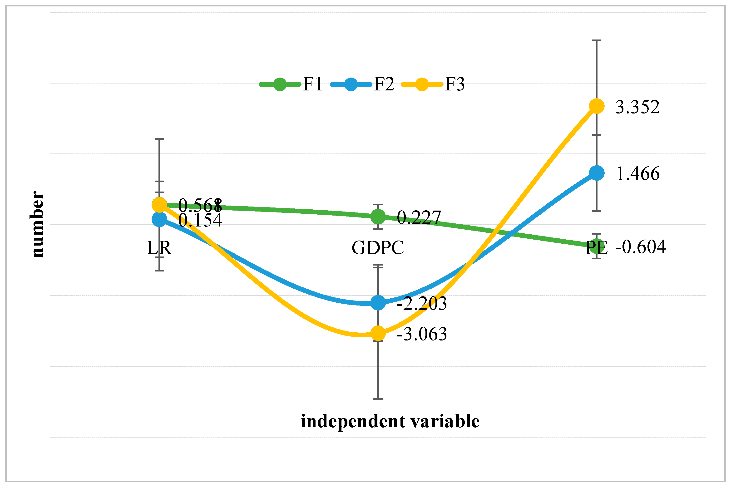
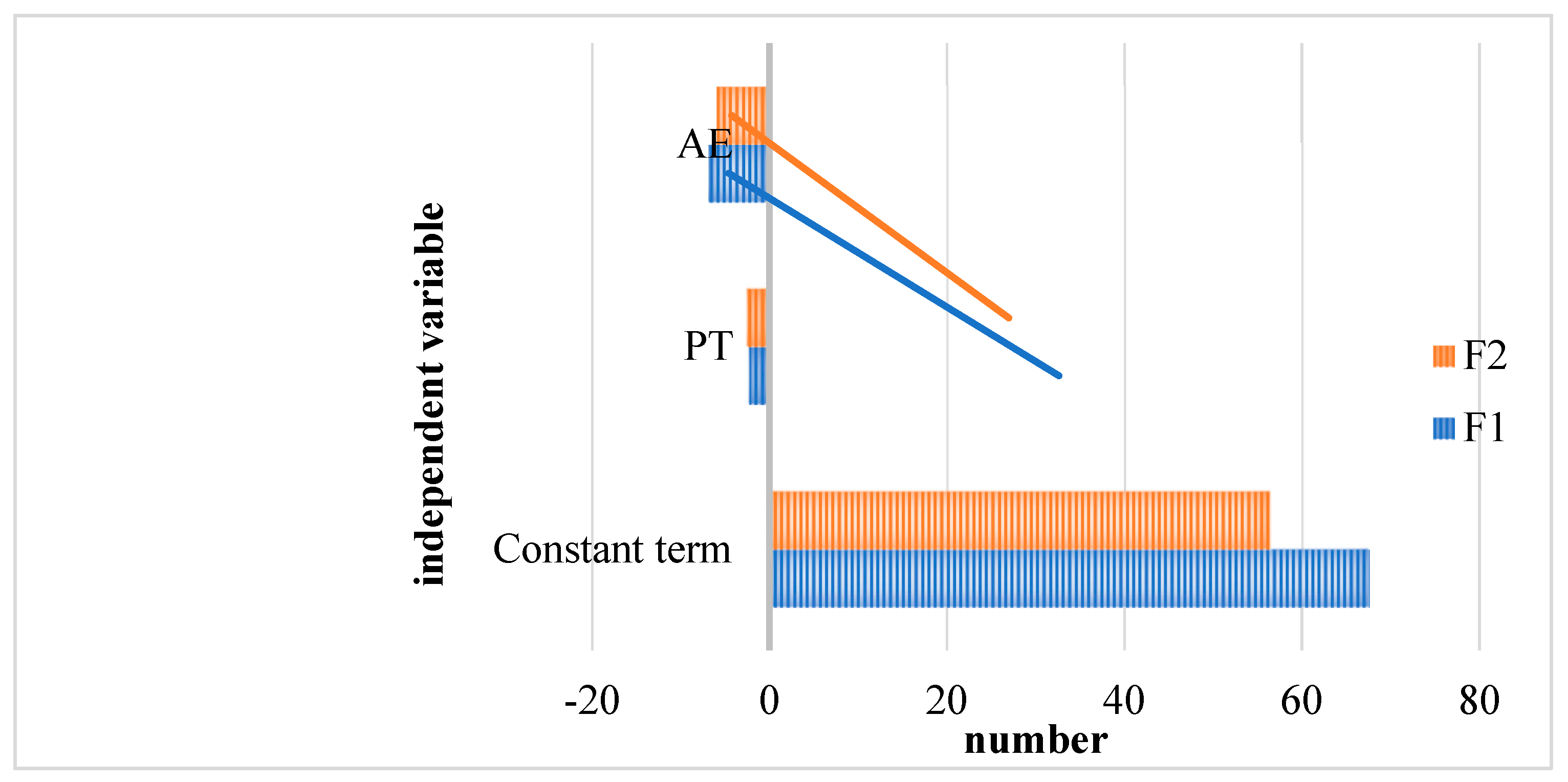
Figure 5 shows the constant items, the post and telecommunications business as a proportion of GDP, the average years of education, and the disaster rate in the second stage of the SFA estimate of the agricultural green ecological system. It can be seen from Figure 5 that the post and telecommunications business as a proportion of GDP had a negative impact on the input slack of basic agricultural investment, environmental protection research investment and government financial support, all reaching a significance level of 5%, which is in line with the expectations of this article. The proportion of post and telecommunications business characterized the regional infrastructure construction. The optimization of infrastructure will lead to a decline in basic agricultural investment, scientific research investment in agricultural environmental protection and government financial support investment slack, which is conducive to resource and energy conservation, and is conducive to green agriculture. The average number of years farmers were in education had a positive impact on the input slack in basic agricultural input and government financial support, reaching significance levels of 1% and 5%, respectively. This result indicates that the higher the average number of years farmers were in education, the lower the efficiency of basic agricultural inputs and government financial support, and the more serious the waste. The impact of the disaster rate on the slack of agricultural basic input was positive, and the impact of the slack of the government’s financial support was negative, reaching a significance level of 10%, which is consistent with the expected situation. Natural disasters caused the loss and waste of agricultural basic input elements; we found that natural disasters have occurred frequently, subsidies for arable land and farmers have increased, and the efficiency of the use of government funds has been improved.

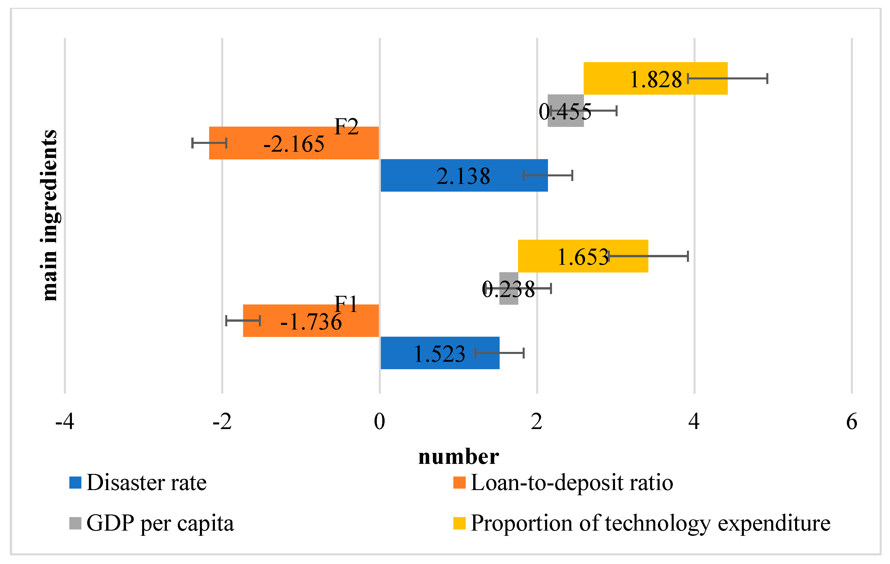
Figure 6 shows the proportions of the loan-to-deposit ratio, GDP per capita and technology expenditure. It can be seen from Figure 6 that the loan-to-deposit ratio had a positive influence on the slack of basic agricultural input. For agricultural production, an increase in the loan-to-deposit ratio indicates that it was easier to obtain funds under a loose financial environment. A smaller capital limit will lead to the increased waste of various basic agricultural inputs and inhibit the efficiency of the agricultural green ecological system. The impact of the per capita GDP on the slack of government financial support was negative, and it passed the 1% statistical significance level. The GDP per capita can represent the level of economic development of a region, indicating that the higher the level of economic development, the higher the level of utilization of government funds in the agricultural production process. These developed regions have taken the lead in the transformation of agricultural development models, with more advanced management concepts and management levels, and the proper use and allocation of funds can promote the efficiency of the agricultural green ecological system. The proportion of science and technology expenditure had a positive impact on the slack of government financial support, reaching a significance level of 1%. This shows that an increase in the proportion of science and technology expenditure will lead to an increase in the waste of government capital investment. A possible reason for this is that there is a longer period between the input and output of science and technology, and the benefits have not been shown. The proportion of science and technology expenditure had a positive impact on environmental protection research investment, but it did not pass the significance test, and a good allocation and operation mechanism has not been established between science and technology expenditure and R&D investment.

5.2. Efficiency Analysis of Agricultural Economic and Social Subsystems

If the technical efficiency level of regional agricultural production is obviously not related to the degree of economic development, it indicates that the research and improvement of technical efficiency have no economic significance, are contrary to economic theory, and are not in line with our actual economic development. China has a vast territory, with large differences in regional natural geographic conditions, economic levels and institutional policies. In order to understand the true agricultural production technology efficiency in each region, we need to conduct the second stage of SFA regression analysis to strip away the infrastructure, labor quality, and natural disaster factors. The financial environment, economic level and government technology supported six environmental factors. The regression results are shown in

Table 4. Constant variables PT, AE, and DR.

Independent Variable	Total Sown Area of Crops	Number of Employed Persons in Rural Areas	Total Power of Agricultural Machinery
Constant term	332.524	721.872	−4321.588
PT	−273.411	−36.543	−46.875
AE	536.187	120.739	487.653
DR	−74.584	−114.996	−6.412

,

Table 5. LR, GDPC and TE.

Independent Variable	Total Sown Area of Crops	Number of Employed Persons in Rural Areas	Total Power of Agricultural Machinery
LR	71.511	35.784	199.524
GDPC	−1158.025	−402.971	−411.845
PT	160.428	115.579	53.847

and

Table 6. Values of ${\delta }^2$ and $\lambda$ in agricultural economic and social subsystems.

Independent Variable	${\mathit{\delta }}^2$	$\mathit{\lambda }$
Total sown area of crops	35.784	199.524
Number of employed persons in rural areas	−402.971	−411.845
Total power of agricultural machinery	115.579	53.847

. The constant items in the SFA estimate of the second stage of the agricultural green ecological system, the proportion of post and telecommunications services in GDP, the average years of education, and the disaster rate are shown in Table 4; the loan-to-deposit ratio, GDP per capita, and the proportion of science and technology expenditures are shown in Table 5. The values of ${\delta }^2$ and $\lambda$ are shown in Table 6.

5.3. Efficiency Analysis of Agricultural Green Ecological Subsystem

Compared to the agricultural economic and social subsystem and the agricultural technology ecological subsystem, the agricultural green ecological subsystem is more constrained by scale efficiency. The same can be seen in the comparison of the four major regions. The technical efficiency of the agricultural green ecological subsystems from high to low were as follows: central, western, eastern and northeastern. Therefore, it was necessary to remove the influence of environmental factors to find its true efficiency level. The constant items, the proportion of post and telecommunications services, and the average years of education in the second stage of the SFA estimate of the agricultural green ecological subsystem are shown in Figure 7. The disaster rate, loan-to-deposit ratio, GDP per capita, and the proportion of science and technology expenditures are shown in Figure 8.

6. Agricultural Green Ecological Efficiency Calculation

Using the data envelopment analysis software Maxdea 6.6 and the unexpected output EBM model combined with the Malmquist–Luenberger index, the changes in the agricultural ecological efficiency in China from 2001 to 2021 were calculated and the results are shown in

Table 7. Results of agricultural ecological efficiency from 2002 to 2021 in China.

2002	2003	2004	2005	2006	2007	2008	2009	2010	2011
0.7340	0.7275	0.7484	0.7442	0.7145	0.7199	0.7849	0.8073	0.7670	0.7694
2012	2013	2014	2015	2016	2017	2018	2019	2020	2021
0.7879	0.8061	0.8191	0.7698	0.8007	0.8170	0.8543	0.8229	0.8963	0.8205

.

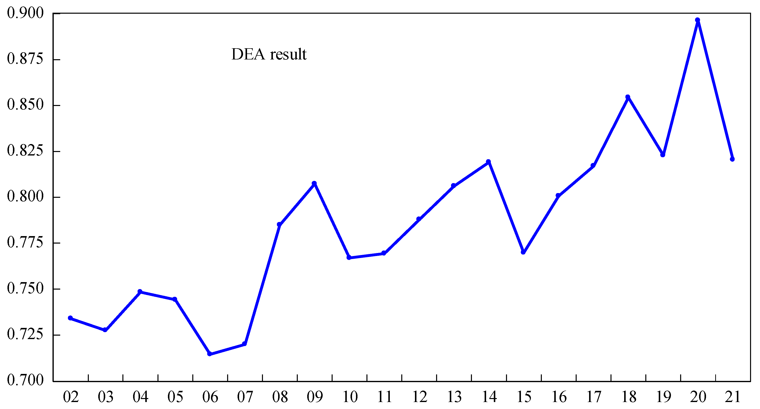
From Figure 9, it can be seen that the agricultural green ecological efficiency increased from 0.7340 in 2002 to 0.8205 in 2021, an increase of 11.78%, showing an overall upward trend. The overall agricultural green ecological efficiency showed an “M” trend of increasing–decreasing–increasing–decreasing–increasing, and a two-stage development pattern in terms of time variation. From 2002 to 2006, the efficiency value decreased from 0.7340 in 2002 to 0.7145 in 2006, a decrease of 2.66%. At this stage, in order to expand agricultural production, investment in agricultural electricity, infrastructure and other factors was increased, which resulted in a significant increase in agricultural carbon emissions. At the same time, there was no timely awareness of the impact of environmental pollution on the agricultural green ecological efficiency and this caused an environmental crisis. From 2007 to 2021, China’s agricultural green ecological efficiency was on a rapid upward trend, with the efficiency value increasing from 0.7199 in 2007 to 0.8205 in 2021, an increase of 13.94%. At this stage, on the one hand, the modern agricultural economic production mode and coordinated development of resources and environment was implemented. On the other hand, there was a growing awareness of the impact of agricultural environment pollution on agricultural green ecological efficiency. Agricultural workers gradually began to pay attention to environmental governance in the process of agricultural planting, which greatly improved the level of agricultural ecological efficiency in China.

7. Discussion

According to the selection requirements for the evaluation index system of agricultural green ecological efficiency mentioned above and based on the DEA model index system, more comprehensive indicators for measuring agricultural green ecological efficiency were selected to be included in the BP neural network model index system. Based on the relevant literature [47], 4 new indicators were added and a total of 13 indicators were selected as input variables for the BP neural network in order to conduct the final evaluation of China’s agricultural green ecology, as shown in

Table 8. BP neural network model indicator system.

	Variable Indicators	Variable Code
Input variables	Total sown area of crops	X1
	Number of employed persons in rural areas	X2
	Total power of agricultural machinery	X3
	Financial expenditure for agriculture	X4
	Forestry and water affairs	X5
	Amount of agricultural fertilizer	X6
	Agriculture electricity consumption	X7
	Agriculture energy input	X8
	Energy promotion manager	X9
	Social development level	X10
	Policy environment	X11
	Economic openness	X12
	Rural communication level	X13

. The indicator system of the BP neural network model was enriched in aspects such as communication factors, social factors, policy environment factors and openness, in order to evaluate China’s agricultural green ecological efficiency from a more comprehensive perspective.

In this section, agricultural green ecological efficiency data from 2001 to 2019 in China were selected as samples for BP neural network training, and the trained network was tested using the 2020 data. After the network test results met the set standard requirements, the final evaluation of the agricultural green ecological efficiency level in 2021 was conducted. This study used the neural network toolbox in MATLAB 2017a software to develop a BP neural network. The parameters were as follows: a three-layer BP network structure, the transfer function between the input layer and the hidden layer used the Logsig function, the transfer function of the output layer used the Purelin function, the learning rate was 0.01, the training function was set to the Trainlm function of the Levenberg–Marquardt algorithm and the number of nodes in the input layer of the BP neural network model was 12. The number of nodes in the hidden layer of the BP neural network model was six and the number of nodes in the output layer was one, i.e., the output efficiency value.

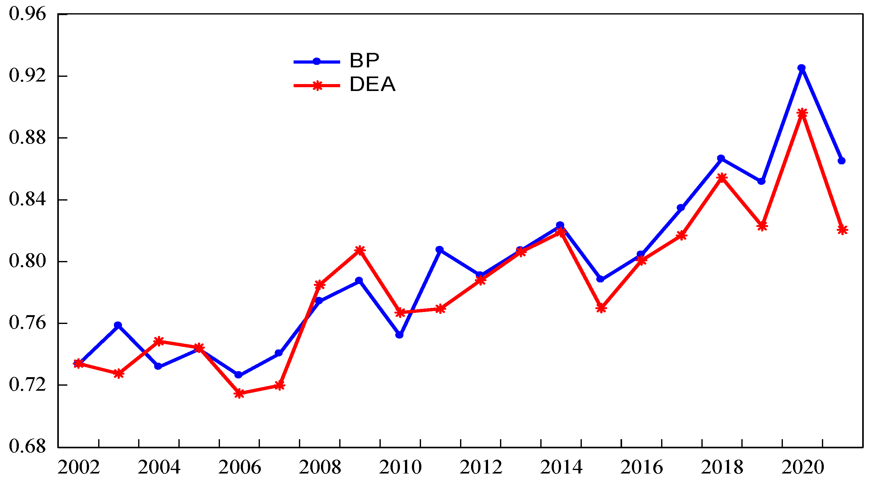
The tested data from 2020 were input into the trained BP neural network model and the effectiveness of the BP neural network model was verified. The results comparing the output of the BP neural network model and the DEA model of the test samples used to fit the true and predicted values are shown in

Table 9. Comprehensive evaluation results of DEA and BP neural network models.

	2002	2003	2004	2005	2006	2007	2008	2009	2010	2011
BP	0.7336	0.7584	0.7317	0.7433	0.7262	0.7403	0.7743	0.7873	0.752	0.8072
DEA	0.7340	0.7275	0.7484	0.7442	0.7145	0.7199	0.7849	0.8073	0.7670	0.7694
	2012	2013	2014	2015	2016	2017	2018	2019	2020	2021
BP	0.7909	0.8071	0.8232	0.7881	0.8043	0.8344	0.8664	0.8514	0.925	0.8648
DEA	0.7879	0.8061	0.8191	0.7698	0.8007	0.8170	0.8543	0.8229	0.8963	0.8205

.

It can be seen from Figure 10 that the results of the BP neural network model were consistent with those obtained by the DEA method, and the overall evolution trend of agricultural green ecological efficiency calculated by the BP neural network also fluctuated and increased. The agricultural green ecological efficiency increased from 0.7336 in 2002 to 0.8648 in 2021, an increase of 17.88%, and showing an overall upward trend. From 2002 to 2006, the efficiency value decreased from 0.7336 in 2002 to 0.7262 in 2006, a decrease of 1.01%. From 2007 to 2021, China’s agricultural green ecological efficiency was on a rapid upward trend, with the efficiency value increasing from 0.7403 in 2007 to 0.8648 in 2021, an increase of 16.82%. Therefore, combining DEA with a BP neural network can correct the evaluation results of agricultural green ecological efficiency. The results obtained via the instance data operations were used as the training dataset for the BP neural network; the effectiveness and accuracy of the BP neural network in evaluating the agricultural green ecological efficiency was verified via comparison with the DEA results. Meanwhile, the comparison between the DEA method and BP neural network calculation showed that the results obtained using the two methods were basically consistent, and these two methods were mutually verified and integrated, which made the evaluation of the agricultural green ecological efficiency more scientific and rigorous.

8. Conclusions

This article started with an overview of the related research and theories of green ecology, defined the concept of agricultural green ecological systems and constructed an efficiency evaluation index system for China’s agricultural green ecological system. The BP neural network and the three-stage DEA model measured the efficiency of the agricultural green ecological system and analyzed its temporal and spatial evolution characteristics. The main conclusions were as follows: (1) the overall technical efficiency of China’s agriculture economic and social subsystems, agricultural science and technology ecological subsystems, and agricultural green ecological subsystems all showed an upward trend. (2) In the agricultural green ecological system, the post and telecommunications business as a proportion of GDP, disaster rate, and per capita GDP had a significant negative impact on the slack of government financial support. The proportion of post and telecommunications business had a significant impact on basic agricultural investment and environmental protection research investment. The impact was also negative, indicating that the optimization of infrastructure, the frequent occurrence of natural disasters and the increase in the level of economic development were conducive to the investment and rational allocation of government funds, and was conducive to the improvement in the efficiency of the agricultural green ecological system. Farmers’ average years of education, the disaster rate, and loan-to-deposit ratio had a positive impact on the slack of basic agricultural inputs. The average number of years farmers were in education and the proportion of science and technology expenditures had a positive impact on the slack of government financial support. The increase in the deposit ratio brought about a loose financial environment and more accessible agricultural funds, which, to a certain extent, led to an increase in the waste of various basic inputs in agriculture.

According to the research results, many managerial insights can be put forward as follows. First, we should accelerate the transformation and upgrading of agricultural technology. The concept of green development should be integrated into agricultural production, and the introduction of advanced agricultural production technologies should be imported. Additionally, the awareness of technological innovation among agricultural workers should be continuously strengthened in order to achieve a significant improvement in agricultural production efficiency. Second, we should improve the financial support for agriculture. By increasing the government’s financial support for the entire agricultural production process, the agricultural sector can update agricultural machinery and improve the construction of agricultural production facilities to effectively enhance the green ecological efficiency of agriculture. Third, we should elevate farmers’ environmental awareness. The concepts of environmental protection and green agriculture development should be strengthened in multiple ways to the public, so that farmers will pay more attention to the relationship between humans and nature to bring about ecological benefits. Fourth, we need to implement ecological subsidy policies. The agricultural ecological subsidy mechanism should be established and improved, and an ecologically oriented subsidy policy system should be built. Moreover, efficient and accurate agricultural subsidy policies should be implemented to realize the transformation of traditional agricultural subsidy policies into ecologically oriented green agriculture subsidy policies.

On the other hand, a BP neural network model was used to evaluate the agricultural green ecology efficiency, and the accuracy of the model results were improved. However, as a composite system, there were many factors that affected agricultural green ecological efficiency, and the further optimization of the evaluation index system is needed in order to better improve the accuracy of the evaluation results in the future.