Volatility Connectedness of Chinese Financial Institutions: Evidence from a Frequency Dynamics Perspective

Abstract

Accurately measuring systemic financial risk and analyzing its sources are important issues. This study focuses on the frequency dynamics of volatility connectedness in Chinese financial institutions using a spectral representation framework of generalized forecast error variance decomposition with the least absolute shrinkage and selection operator vector autoregression. It assesses the volatility connectedness network using complex network analysis techniques. The data are derived from 31 publicly traded Chinese financial institutions between 4 January 2011 and 31 August 2023, encompassing the Chinese stock market crash in 2015 and the COVID-19 pandemic. The frequency dynamics of the volatility connectedness results indicate that long-term connectedness peaks and cross-sectoral connectedness rises during periods of financial instability, especially in the recent bull market (2014–2015) and the 2015 Chinese stock market crash. The volatility connectedness of Chinese financial institutions declined during the COVID-19 pandemic but rose during the post-COVID-19 pandemic period. Network estimation results show that securities triggered the 2015 bull market, whereas banks were the main risk transmitters during the 2015 market crash. These results have important practical implications for supervisory authorities.

1. Introduction

The connectedness of financial institutions is an important trigger for the accumulation, propagation, and spread of systemic financial risks. Since the 2008 global financial crisis, considerable attention has been directed toward financial entities’ connectedness because institutions are dubbed “too connected to fail” [1,2,3]. Shocks considered insignificant, such as those that affect only a few institutions or markets at an early stage, can spread across highly interconnected financial institutions, eventually affecting the entire financial system [4,5].

As China increases its position as the second leading country in the global financial system, its financial system has increasingly been under scrutiny via global markets. This is also due to China’s rapid economic growth and the Chinese stock market crash that occurred in 2015 [6,7]. After the financial crisis, global systemically important banks (G-SIBs) shifted from developed to emerging economies like China [8]. Five Chinese financial institutions—the Agricultural Bank of China (ABC), Bank of China (BOC), China Construction Bank (CCB), Industrial and Commercial Bank of China Ltd. (ICBC), and Ping An Insurance (Group) Co. of China, Ltd. (PAI)—have been included on the G-SIB list since 2011 and the list of global systemically important insurers (G-SIIs) since 2014. This implies that China is a significant player in the global financial system. Thus, gauging and comprehending connectedness in China’s financial system is vital for prudential authorities in China and the global financial system.

Research examining volatility connectedness across diverse financial markets and institutions has steadily increased. For example, there have been numerous studies conducted on international stock markets [9,10,11], commodity markets [12,13], gold markets [14,15], global sovereign credit default swaps [16,17], exchange rate markets [18,19,20], cryptocurrencies [21,22,23], and crude oil, gold, and stock markets [24,25].

The connectedness of financial institutions in China has received much attention from scholars. Some studies use the tail-event driven network (TENET) approach [26] to investigate the financial institutions in China affected by the extreme risk spillover network [27], some studies apply decomposed returns and the Granger causality test to measure the systematic and idiosyncratic networks of financial institutions in China [7], some studies [28] use the Diebold–Yilmaz method [29] to examine volatility connectedness among 14 publicly traded commercial banks in China, and some studies [30] investigate the frequency dynamics of connectedness among financial institutions in China using the Baruník–Křehlík method [31].

The spread of COVID-19, which began in January 2020, had a huge impact on global financial markets within a short period of time [32]. The outbreak of the COVID-19 pandemic led to higher non-performing loan rates for banks [33], premium income declined for insurance [34], the index for the stock market declined, and the entire financial market was in a state of shock [35]. Although some studies have explored the impact of COVID-19 on the volatility connectedness of global stock markets [36], dominant agricultural commodity markets [37], cryptocurrencies, and fiat currencies [38], there has been a lack of attention paid to the impact of COVID-19 on the volatility connectedness of Chinese financial institutions.

Methodological aspects of the connectedness index based on vector autoregression (VAR) have been widely used in the economic and financial literature [23]. Among them, Diebold and Yilmaz’s time-domain method [29], based on the variance decomposition of prediction error, has attracted much attention and been applied to stock, crude oil, bond market connectedness, and so on [39,40,41]. To extend connectedness, a new time-frequency connectedness method to decompose the spillover results has been proposed [31], which places variables that were originally in the time domain into different frequency domains, thus revealing differences in spillover levels at different cycle lengths. The most recent studies on frequency connectedness [42,43,44] employ the new approach proposed by Baruník and Křehlík [31]. The model proposed by Diebold and Yilmaz deals only with the time domain, whereas the method proposed by Baruník and Křehlik enables the assessment of connectedness by simultaneously considering both magnitude and directionality features concerning time and different frequencies. Hence, unlike the aggregate time-variant information used in the Diebold–Yilmaz method [45], aggregate connectedness is decomposed into different frequency domains using the method proposed by Baruník and Křehlík. Distinguishing between short- and long-term connectedness is important because recent research emphasizes that connectedness in markets pertinent to finance and commodities varies with diverse degrees of persistence [46,47]. For example, when portfolio construction is a concern, investors with long (short) investment perspectives may pay attention to the long-run (short-run) volatility connectedness between institutions. Moreover, high long-run volatility connectedness across diverse institutions implies the persistence of a long-term impact on the system. Therefore, policymakers should concentrate on shocks that increase long-run volatility connectedness across financial institutions, as such shocks would have a long-run effect on the system.

This study employs the connectedness methodology proposed by Baruník and Křehlík to assess the time and frequency of the dynamic connectedness of 31 Chinese financial institutions. This study contributes to the literature in the following ways. First, the previous literature evaluated the connectedness of financial institutions only in the time domain [27,40,41,48], whereas we distinguish the connectedness among institutions at different frequencies over different periods. This is an important distinction since our results indicate that the significance of an institution as a target or source of risks depends on the frequency and period. In addition, we examine the connectedness of all financial institutions, including banks, insurers, and securities, whereas some studies consider only banks [28]. Second, we utilize Baruník and Křehlík’s advantageous approach [31] in different sectors to analyze the connectedness of 31 publicly traded Chinese financial institutions at three different frequencies (short-, medium-, and long-term). Our approach is like some recent works [30,49] that surveyed the connectedness of different financial institutions but did not analyze the network structure of connectedness in depth. Our approach further explores the frequency connectedness network graphs to understand the underlying network structure better. Third, the data span for our study encompasses not only the Chinese stock market crash in 2015 but also the outbreak of COVID-19 in 2020, during which financial markets experienced extreme volatility.

Finally, we found that both long-term and cross-sectoral connectedness reached a maximum as system stability faced uncertainty or distress, especially during the recent bullish period (2014–2015) and the 2015 Chinese stock market crash. Hence, long-run connectedness can be utilized as an early alert indicator by regulators monitoring distress in the system. Moreover, when cross-sectoral connectedness increases, regulatory commissions should focus on cross-sectoral connectedness and increase their efforts to coordinate administrative abilities.

The remainder of the paper is organized as follows. Section 2 presents the methodology. Section 3 presents the data that have been employed. Section 4 presents the empirical results and discussion. Finally, Section 5 presents our conclusions.

2. Methodology

We employ the connectedness methodology proposed by Baruník and Křehlík to assess the time and frequency of the dynamic connectedness of 31 Chinese financial institutions, which we considered to prolong the time-frequency aspect of the Diebold–Yilmaz connectedness approach.

The method proposed by Diebold and Yilmaz uses forecasting error variance decomposition under the generalized VAR model introduced by Koop et al. [50] and Pesaran and Shin [51] to obtain predictions related to both the magnitude and direction of connectedness in the global financial system within the time domain. The spectral representation of variance decompositions was included in the Diebold–Yilmaz approach by Baruník and Křehlík as an extension of the method [47,52], thus simplifying the estimation of unconditional connectedness relations in the frequency domain. Hence, the Baruník–Křehlík approach provides the distinctive feature of gauging the dynamics of connectedness among a set of variables that consider time and frequencies simultaneously.

2.1. Diebold–Yilmaz Time-Domain Connectedness

The VAR(p) model, expressed as $y_t={{\displaystyle \sum }}_{i=1}^p{\Phi }_i{y}_{t-i}+{\epsilon }_t$, consisting of N variables, is first estimated when the Diebold–Yilmaz approach is implemented. As the number of variables increases, the parameters to be estimated increase quadratically because the VAR model is over-parameterized. This causes a high probability of observing a “dimensional disaster”. Overparameterization makes the VAR model unable to estimate more variables, which is why Diebold and Yilmaz [29] chose only 13 financial institutions when studying the volatility spillover effect in the U.S. The current study examines 31 financial institutions. When the lag order p = 5 for the VAR model is chosen, 4836 parameters must be estimated. However, the traditional VAR model cannot estimate them accurately.

To overcome this problem, we estimate VAR(p) using an extended version of the least absolute shrinkage and selection operator vector autoregression (LASSO-VAR) framework proposed by Nicholson et al. [53]. Moreover, we applied Simon et al. [54]’s sparse-group LASSO method, which considers sparse effects at both the group and intragroup levels.

By using the moving average model, the VAR(p) can be defined as follows: $Y_t={{\displaystyle \sum }}_{j=1}^{\infty }{\Psi }_j{\epsilon }_{t-j}$, where ${\Psi }_j={\Phi }_1{\Psi }_{j-1}+{\Phi }_2{\Psi }_{j-2}+\cdots +{\Phi }_p{\Psi }_{j-p}$, where ${\Psi }_0$ is an identity matrix of dimension $N\times N$ and ${\Psi }_j$ is a zero matrix for $j<0$.

Diebold and Yilmaz’s [45] generalized variance decomposition (GVD) VAR method was employed, independent of variable ordering. Variable k contributes to variable j using H-step-ahead generalized forecast error variance expressed as

$${\theta }_{jk}^H=\frac{{\sigma }_{kk}^{-1}{{\displaystyle \sum }}_{h=0}^{H-1}{\left({e^{\prime }}_j{\Psi }_h\Sigma e_k\right)}^2}{{{\displaystyle \sum }}_{h=0}^{H-1}\left({e^{\prime }}_j{\Psi }_h\sum {{\Psi }^{\prime }}_h{e}_j\right)}$$

(1)

The covariance matrix for the error vector $\epsilon$ is denoted by $\mathsf{\Sigma }$, the standard deviation of the error term in the kth equation is denoted by ${\sigma }_{kk}$, a selection vector with the jth and kth elements equal to 1 and the rest equal to 0 s are denoted by $e_j and e_k$, respectively, and the variance matrix of the error vector $\epsilon$ is denoted by Σ. Because orthogonality may not be satisfied by shocks in the GVD framework, the sum of the forecast error variance is not necessarily equal to one. Hence, each element of the H-step-ahead GVD matrix is normalized by the summation of the row sum, that is,

$${\tilde{\theta }}_{jk}^H=\frac{{\theta }_{jk}^H}{{{\displaystyle \sum }}_{k=1}^N{\theta }_{jk}^H}$$

(2)

where ${{\displaystyle \sum }}_{j=1}^N{\tilde{\theta }}_{jk}^H=1$ and ${{\displaystyle \sum }}_{i,j=1}^N{\tilde{\theta }}_{jk}^H=N$ followed by the construction. ${\tilde{\theta }}_{jk}^H$ is the pairwise directional connectedness ranging from attributes k to j; that is, if ${\tilde{\theta }}_{jk}^H$ is positive, then attribute k generates connectedness with variable j.

To analyze the network’s topological properties, three connectivity measurement categories were selected: (i) system-wide connectivity, (ii) sector-conditional connectivity, and (iii) institutional-level connectivity.

From an overall system perspective, the total connectedness (TC), expressed as the portion of the variance in the forecasts that its errors contribute by themselves, was computed. The ratio of the summation of the off-diagonal elements in the normalized GVD matrix is given by Equation (3):

$$TC=\frac{{{\displaystyle \sum }}_{j\ne k}{\tilde{\theta }}_{jk}^H}{N}$$

(3)

Moreover, four measurements regarding the strength of sector-conditional connectivity were introduced. When focusing on a certain sector, we can obtain measurements such as the total connectedness within the sector, directional connectedness from the sector to others or from others to the sector, and the net directional connectedness of the sector. For sector M, these indicators are $T{C}_M$, $IN\_D{C}_M$, $OUT\_D{C}_M$, and $NET\_D{C}_M$, and they were computed as follows:

$$T{C}_M=\frac{{{\displaystyle \sum }}_{j\ne k,j,k\in M}{\tilde{\theta }}_{jk}^H}{N_M\times \left(N_M-1\right)}$$

(4)

$$IN\_D{C}_M=\frac{{{\displaystyle \sum }}_{j\in M,k\notin M}{\tilde{\theta }}_{jk}^H}{N_M\times \left(N-N_M\right)}$$

(5)

$$OUT\_D{C}_M=\frac{{{\displaystyle \sum }}_{j\in M,k\notin M}{\tilde{\theta }}_{kj}^H}{N_M\times \left(N-N_M\right)}$$

(6)

$$NET\_D{C}_M=OUT\_D{C}_M-IN\_D{C}_M$$

(7)

where the total number of financial institutions in the system and sector M is denoted by $N$ and $N_M$, respectively, and thus, the number of other sectors is denoted by $N-N_M$. Considering sector M as a subsystem, the higher the total connectedness, the more intense the risk spillover among institutions in the sector. Additionally, $IN\_D{C}_M$, $OUT\_D{C}_M$, and $NET\_D{C}_M$ represent the significance of sector M for risk reception, risk transmission, and net risk spillover, respectively.

Regarding institutional-level connectivity, to assess the significance of individual financial institutions in risk transmission (reception), three directional measures of institutional strength, $IN\_S_j$ and $OUT\_S_j$ representing the directional connectedness from institution j to others and from others to institution j, respectively, and $Net\_S_j$, which represents the net directional connectedness of institution j, are denoted by

$$IN\_S_j={\displaystyle \sum }_{k=1,j\ne k}^N{\tilde{\theta }}_{jk}^H$$

(8)

$$OUT\_S_j={\displaystyle \sum }_{k=1,j\ne k}^N{\tilde{\theta }}_{kj}^H$$

(9)

$$Net\_S_j=IN\_S_j-OUT\_S_j$$

(10)

2.2. Baruník–Křehlík Frequency-Domain Connectedness

Following Dew-Becker and Giglioi’s work [55], as proposed by Baruník and Křehlík [31], a frequency response function can be obtained by using the moving average coefficients ${\Psi }_h$, to which Fourier transform is applied, that is, $\Psi \left(e^{-i\omega }\right)={{\displaystyle \sum }}_h{e}^{-i\omega h}{\Psi }_h$, where $\omega$ denotes the frequency and $i=\sqrt{-1}$. The associated power spectrum $S_Y\left(\omega \right)$ represents the distribution of $y_t$ over the frequency components $\omega$ and is denoted by $S_Y\left(\omega \right)={{\displaystyle \sum }}_{h=\infty }^{\infty }E\left(y_{t}y{\prime }_{t-h}\right)e^{-i\omega h}=\Psi \left(e^{-i\omega }\right)\Sigma \Psi \prime \left(e^{+i\omega }\right)$.

Employing the frequency response functions from the spectral representation helps derive the GVD in the frequency domain. Thus, the generalized forecast error variance decomposition (GFEVD) at a particular frequency $\omega$ was calculated as follows:

$${\theta }_{jk}\left(\omega \right)=\frac{{\sigma }_{kk}^{-1}{\left|\Psi \left(e^{-i\omega }\right)\Sigma \right|}_{j,k}^2}{{\left(\Psi \left(e^{-i\omega }\right)\Sigma {\Psi }^{\prime }\left(e^{+i\omega }\right)\right)}_{jj}}$$

(11)

where ${\theta }_{jk}\left(\omega \right)$ is the proportion of the spectrum of the jth variable at a given frequency $\omega$ that can be attributed to shocks in the kth variable. To extract frequencies from the natural decomposition of the original GFEVD, a weight was assigned to ${\theta }_{jk}\left(\omega \right)$ concerning the frequency portion of the variance of the jth variable. The weighting function can be expressed as

$${\Gamma }_j\left(\omega \right)=\frac{{\left(\Psi \left(e^{-i\omega }\right)\Sigma {\Psi }^{\prime }\left(e^{+i\omega }\right)\right)}_{jj}}{\frac{1}{2\pi }{{\displaystyle \int }}_{-\pi }^{\pi }{\left(\Psi \left(e^{-i\omega }\right)\Sigma {\Psi }^{\prime }\left(e^{+i\omega }\right)\right)}_{jj}d\lambda }$$

(12)

which represents the power of the jth variable at a given frequency and sums the frequencies to a constant value of $2\pi$. For a frequency band given by $d=\left(a,b\right), a,b\in \left(-\pi ,\pi \right), a<b$, the GFEVD on frequency band $d$ is expressed as ${\theta }_{jk}^d=\frac{1}{2\pi }{{\displaystyle \int }}_a^b{\Gamma }_j\left(\omega \right){\theta }_{jk}\left(\omega \right)d\omega$. Then, the scaled GVD is defined in frequency band $d$ as

$${\tilde{\theta }}_{jk}^d={\theta }_{jk}^d/{\displaystyle \sum }_k{\theta }_{jk}^{\infty }$$

(13)

where ${\tilde{\theta }}_{jk}^d$ measures the percentage of forecast error variation for variable k due to shocks to variable j at a specific frequency band $d$, and ${\theta }_{jk}^{\infty }$ is the GFEVD of the entire range of the frequencies.

The total connectedness at frequency band d can be denoted by:

$$T{C}^d=\frac{{{\displaystyle \sum }}_{j\ne k}{\tilde{\theta }}_{jk}^d}{\sum {\tilde{\theta }}_{jk}^{\infty }}$$

(14)

The original connectedness is decomposed into distinct parts by the frequency connectedness. When the summation was conducted, the total connectedness, TC, expressed by Diebold and Yilmaz [29], was equal to this summation. Equations (4)–(7) and Equations (8)–(10) define a similar sector and directional frequency connectedness in the frequency domain.

2.3. Graphical Display of Network

In the analysis, 31 nodes and 312 edges were obtained in the graphs, consisting of the entire network, with all these edges hiding the basic figures in the network structure. Hence, network graphs only denote the thickest edges, which is merely a visual choice. Statistics related to all the networks were computed using the full network.

Following Bostanci and Yilmaz [16] and Demirer et al. [56], Gephi open-source software was used to construct, visualize, and analyze voluminous network graphs. Color, size, and locations for nodes and thickness and color for edges were employed for additional and hard-to-spot information.

The node color indicates the node sector. Nodes representing financial institutions with outgoing edges in the same sector have the same color. Green, red, and yellow indicate banks, securities, and insurers, respectively.

The to-connectedness of a node is indicated by its size. Each node’s radius is proportional to the to-connectedness of its corresponding financial institution. A larger node size denotes the institutions with a larger overall influence.

The pairwise direction is indicated by edge thickness and color. The thickness of the edge from nodes i to j increases with the pairwise directional connectedness from nodes i to j. The lighter color for edges shows the weakest links; the same is true for all other links.

The ForceAtlas2 algorithm created by Jacomy et al. [57] was employed to determine node locations implemented in Gephi. According to the algorithm, the nodes repulse each other, except for the connected nodes. In the algorithm, a steady state is reached when the repelling and attracting forces balance each other exactly for every pair of nodes, as determined by the average pairwise directional connectedness between the two nodes. Nodes with higher pairwise directional connectedness values are expected to be closer to each other in the steady state.

3. Data

We analyzed the daily trading data of all publicly traded financial institutions listed in China’s A-share market before 2011, and the data were downloaded from Wind Info between 4 January 2011, and 31 August 2023, which covered the Chinese stock market crash in 2015. Hence, the sample includes 3 insurers, 16 banks, and 12 securities.

Table 1. Descriptive statistics.

Ticker Code	Financial Institution	Abbr.	Mean	Std. Dev.	Skewness	Kurtosis	ADF
Panel A: Insurance
601318.SS	Ping An Insurance	PAI	0.0007	0.0009	6.26	77.92	−32.093 ***
601601.SS	China Pacific Insurance	CPIC	0.0009	0.0010	3.84	27.47	−30.876 ***
601628.SS	China Life Insurance	CLI	0.0009	0.0012	4.494	33.34	−26.268 ***
Panel B: Banks
000001.SZ	Ping An Bank	PAB	0.0008	0.0010	4.396	38.06	−29.637 ***
002142.SZ	Bank of Ningbo	NBCB	0.0009	0.0012	5.318	58.05	−29.107 ***
600000.SS	Shanghai Pudong Development Bank	SPDB	0.0005	0.0008	4.126	28.63	−28.839 ***
600015.SS	Hua Xia Bank	HXB	0.0006	0.0009	5.258	50.37	−26.748 ***
600016.SS	China Minsheng Banking	CMBC	0.0006	0.0010	5.216	45.88	−26.147 ***
600036.SS	China Merchants Bank	CMB	0.0007	0.0009	6.173	69.85	−27.399 ***
601009.SS	Bank of Nanjing	NJBK	0.0007	0.0011	5.239	48.79	−27.117 ***
601166.SS	Industrial Bank	CIB	0.0006	0.0009	4.146	28.56	−29.045 ***
601169.SS	Bank of Beijing	BOB	0.0005	0.0009	4.844	39.34	−26.741 ***
601288.SS	Agricultural Bank of China Limited	ABC	0.0004	0.0007	5.547	47.02	−27.599 ***
601328.SS	Bank of Communications	BOCOM	0.0005	0.0009	6.084	56.98	−23.255 ***
601398.SS	Industrial and Commercial Bank of China	ICBC	0.0004	0.0007	7.051	81.36	−26.930 ***
601818.SS	China Everbright Bank	CEB	0.0006	0.0010	6.783	81.79	−26.274 ***
601939.SS	China Construction Bank Corporation	CCB	0.0005	0.0008	6.423	71.23	−25.285 ***
601988.SS	Bank of China Limited	BOC	0.0004	0.0009	7.442	80.89	−24.330 ***
601998.SS	China CITIC Bank Corporation Limited	CNCB	0.0007	0.0012	4.49	32.83	−26.976 ***
Panel C: Securities
000686.SZ	Northeast Securities	NESC	0.0011	0.0015	3.669	26.61	−29.014 ***
000728.SZ	Guoyuan Securities	GYSC	0.0011	0.0016	4.179	32.13	−27.186 ***
000776.SZ	GF Securities	GFSC	0.0010	0.0014	4.615	44.75	−28.925 ***
000783.SZ	Changjiang Securities	CJSC	0.0010	0.0015	4.829	44.68	−28.038 ***
600030.SS	CITIC Securities	CITICS	0.0009	0.0013	4.42	37.03	−28.984 ***
600109.SS	Sinolink Securities	SLSC	0.0013	0.0017	3.992	32.11	−29.332 ***
600837.SS	Haitong Securities	HTSEC	0.0009	0.0012	3.666	24.51	−30.530 ***
600999.SS	China Merchants Securities	CMSC	0.0010	0.0014	4.636	41.99	−26.952 ***
601099.SS	The Pacific Securities	PSC	0.0012	0.0016	3.737	26.29	−28.644 ***
601377.SS	Industrial Securities	CISC	0.0011	0.0015	4.272	37.63	−30.085 ***
601688.SS	Huatai Securities	HTSC	0.0010	0.0014	4.281	35.98	−27.371 ***
601788.SS	Everbright Securities	EBSCN	0.0011	0.0015	4.251	35.39	−27.821 ***

Note: ADF, augmented Dickey–Fuller test, null hypothesis of a unit root in each volatility series, *** indicates rejection of the null hypothesis at the 1% significance level; PAI, Ping An Insurance (Group) Co. of China, Ltd.; ABC, Agricultural Bank of China; BOC, Bank of China; CCB, China Construction Bank; ICBC, Industrial and Commercial Bank of China Ltd.

shows detailed information for each.

Following Diebold and Yilmaz [29] and Wang et al. [28], Garman and Klass’s range-based volatility estimator is employed as follows [58]:

$$V_{it}^{GK}=0.511{\left(H_{it}-L_{it}\right)}^2-0.019\left[\left(C_{it}-O_{it}\right)\left(H_{it}+L_{it}-2O_{it}\right)-2\left(H_{it}-O_{it}\right)\left(L_{it}-O_{it}\right)\right]-0.383{\left(C_{it}-O_{it}\right)}^2$$

(15)

where $H_{it}$,$L_{it}$,$O_{it}$, and $C_{it}$ are the natural logarithms of the daily high, low, opening, and closing prices of institution $i$ on day $t$, respectively. Table 1 presents the summary statistics for the volatility series of the 31 financial institutions during the sample period. The largest mean and standard deviation values are observed in the securities volatility series, which implies that the stock prices of securities are more volatile than those of commercial banks and insurers. According to statistics generated by the augmented Dickey–Fuller test (ADF), being significant at the 1% level implies that stationarity exists in all volatility series; thus, they can be used for VAR modeling.

4. Empirical results

4.1. Dynamic Analysis

4.1.1. Total Frequency Connectedness

Variance decompositions, represented by spectral representations, derive the dynamics of volatility connectedness related to time frequency within a moving window of approximately one year (250 business days). For our final model specification, VARs using the lag group LASSO with the lag order $p=5$ and the predictive horizon H = 100 days were estimated 1. The dynamics of total connectedness concerning time in our system are gauged by variance decompositions of the time domain, as shown in Figure 1. The outcomes concerning the decomposition of total connectedness into frequency bands of up to one week, one week to one month, and one month to one hundred days are shown in Figure 2. The bands computed as $T{C}^d$ corresponding to the short-, medium-, and long-run are denoted by $d_1\in \left[1,5\right], d_2\in \left(5,20\right], d_3\in \left(20,100\right]$ periods, respectively.

First, we focus on the total connectedness, as shown in Figure 1. On average, the total connectedness of the 31 Chinese financial institutions is quite large, at above 70%. Additionally, total connectedness is time-varying and informative. Four prominent cycles with higher total connectedness values were observed. The first cycle started at the end of 2012 and ended in mid-2014, when China’s economic growth began to slow, and severe industrial overcapacity led to a surge in non-performing loans from commercial banks. Then, China’s commercial banks faced two “money shortage” events in June and December 2013 called “the Chinese banking liquidity crisis of 2013.” During this period, China’s financial system’s volatility connectedness and systemic risk increased significantly. The second cycle lasted from mid-2014 to August 2016, when total connectedness rose from 86% to 94% and remained above 91% until August 2016. Subsequently, total connectedness continued to fall to its lowest point of 85% from mid-2016 to the end of 2017. During this cycle, two turning-point events took place in the Chinese stock market: (i) the bull market on the Chinese stock exchange from mid-2014 to June 2015 and (ii) the 2015 Chinese stock market crash and the “Chinese stock market turbulence” in early 2016. From the end of 2014 to June 2015, financial institutions infused large amounts of funds into the stock market by participating in highly leveraged over-the-counter transactions. This excessive risk-taking behavior led to a significant increase in total connectedness. The third cycle ran from mid-2018 to the second half of 2019, during which total connectedness rose rapidly in 2018. This increase can be attributed to the Sino–U.S. trade war and China’s deleveraging strategy. The fourth cycle ran from early 2020 to 2023; in light of the COVID-19 pandemic, it is difficult for Chinese financial institutions to do business, and they are fragmented, which leads to a decline in volatility connectedness among Chinese financial institutions. With the end of the COVID-19 pandemic, the curvilinear rebound from the bottom in early 2022, which shows a recovery of volatility connectedness among Chinese financial institutions.

Figure 2 displays the frequency dynamics of the total connectedness based on time when looking at the frequency components. The decomposition provided the first observation that the periods with high total connectedness were mostly caused by the long-run components (d3). In particular, we noted that the long-run components in the 2015 cycle were much higher than those in the other cycles. Intuitively, the only systemic risk event during the sample period was the 2015 Chinese stock market crash. Another concern is that during the COVID-19 pandemic (2020–2021), although the total connectedness did not change significantly and may even be in a downward cycle, the long-term component increased, indicating that the risk of long-term association increased during this period. Connectedness typically arises during a crisis, implying that long-term connectedness carries a substantial risk of propagation, as rising stock market price volatility accompanies the overall high uncertainty regarding the financial system during these periods. Subsequently, more persistent investor responses to shocks are observed when uncertainty increases. Thus, when a financial system has high connectedness, long-term responses to shocks translate into long-term uncertainty, increasing systemic risk during these periods.

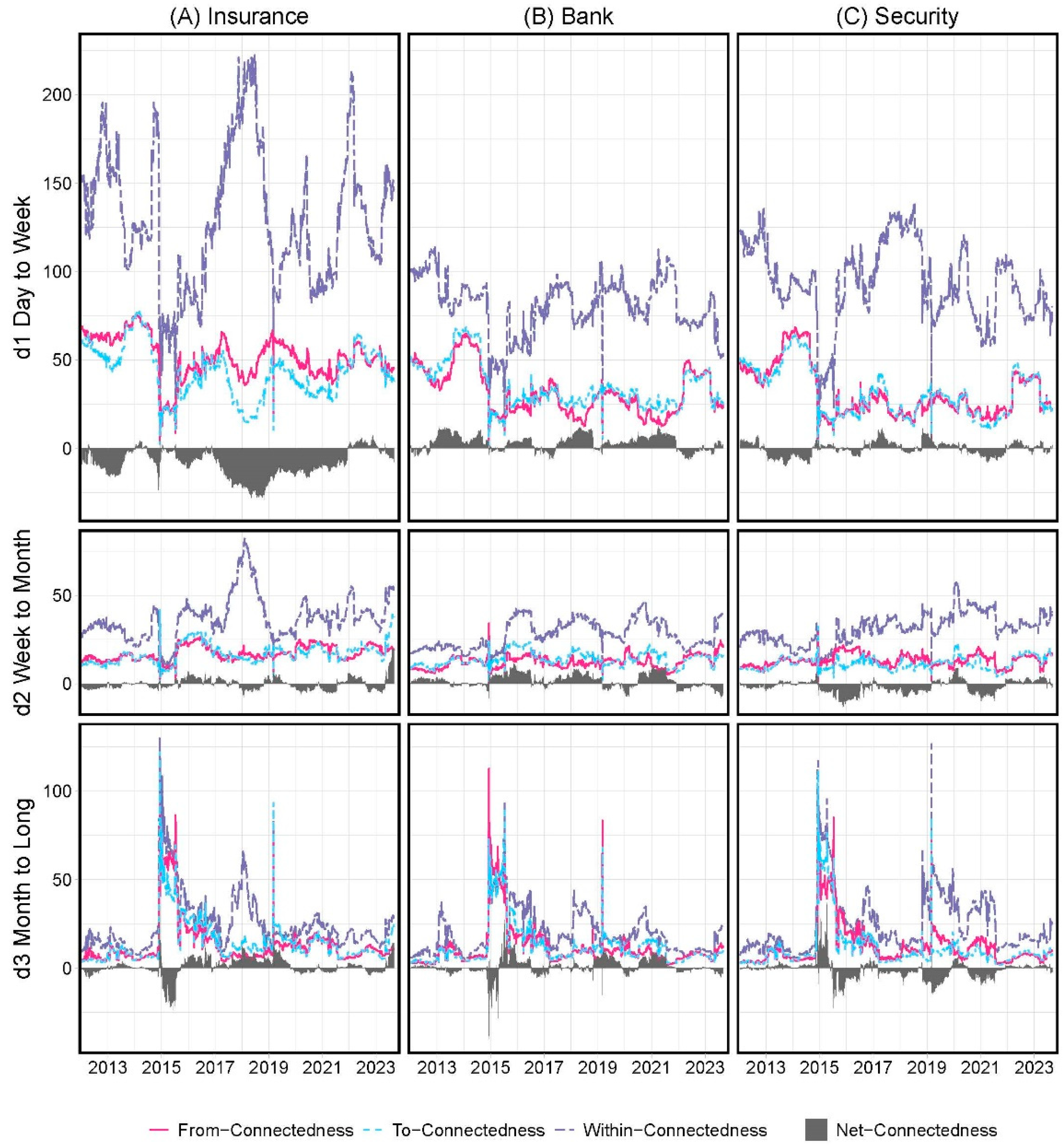
4.1.2. Sector Directional Frequency Connectedness

Thus far, total connectedness and its frequency components have been the focus of our empirical research. Although Figure 1 and Figure 2 provide detailed information, sector-frequency connectedness provides more valuable results. Thus, we examine the time dynamics of connectedness in classified sectors, including insurance, banking, and securities.

Figure 3 shows the evolution of the total connectedness of (each) sector $T{C}_M$, the directional connectedness from (each) sector to others $OUT\_D{C}_M$, or from others to (each) sector $IN\_D{C}_M$, and the net directional connectedness of (each) sector $NET\_D{C}_M$. Throughout the sample period, intra-sector connectedness ($T{C}_M$) was always higher than cross-sector connectedness ($OUT\_D{C}_M$ and $IN\_D{C}_M$). This implies that the connectedness between institutions in the same sector was generally high, indicating that the trends and levels of $T{C}_M$, $OUT\_D{C}_{M,}$ and $IN\_D{C}_M$ in different sectors were identical. Specifically, compared with Figure 1, the cross-sector connectedness and total connectedness trends in Figure 3 are consistent, whereas the intra-sector connectedness and total connectedness trends are the opposite. Thus, the TC trend was caused by cross-sector connectedness. Additionally, net directional connectedness, $NET\_D{C}_M$, was quite different for (each) sector. The banking sector, experiencing positive net directional connectedness, implies that connectedness from the banking sector to other sectors was greater than that from other sectors. Note that the banking sector turned out to be the fundamental risk sender in the system because its net directional connectedness was not only the highest but also the most positive type of connectedness in most phases (e.g., “the Chinese banking liquidity crisis of 2013”, “Chinese stock market crash in 2015”, “Sino-U.S. trade war in 2018”, and “COVID-19 in 2020”).

Next, the results in Figure 4 show the evolution of both the total and directional connectedness of (each) sector based on a frequency dynamics perspective regarding the frequency connectedness of (each) sector (including. $T{C}_M^{d_s}$,$OUT\_D{C}_M^{d_s}$,$IN\_D{C}_M^{d_s},$ and $NET\_D{C}_M^{d_s}$). Similar to the above results, the trends and levels of $T{C}_M^{d_s}$,$OUT\_D{C}_M^{d_s}$, and $IN\_D{C}_M^{d_s}$ in the different sectors were the same. This indicates that after the risk is generated, it quickly propagates among sectors in a highly connected system. Long-term connectedness (d₃) increases during the three abovementioned cycles (especially during the second cycle). Intra-sector connectedness was significantly higher than cross-sector connectedness in the short- and medium-term (d₁ and d₂, respectively). However, there were some exceptions in the long-term. The connectedness within banks was higher than the cross-sector connectedness during the 2015 cycle. These findings suggest that long-term cross-sector connectedness may appear when a systemic problem occurs (e.g., connectedness behavior in the second cycle), thereby increasing systemic risk and endangering system stability. Although the trends of $T{C}_M^{d_s}$,$OUT\_D{C}_M^{d_s}$, and $IN\_D{C}_M^{d_s}$ were similar in different sectors, net frequency connectedness varied significantly. In the long-term, the securities sector was the main risk sender during the first half of 2015, whereas the banking sector was the main risk transmitter during the second half of 2015. Since the 2015 Chinese stock market crash on 15 June 2015, the securities sector has played an important role. The banking sector served as the net risk sender during the crash.

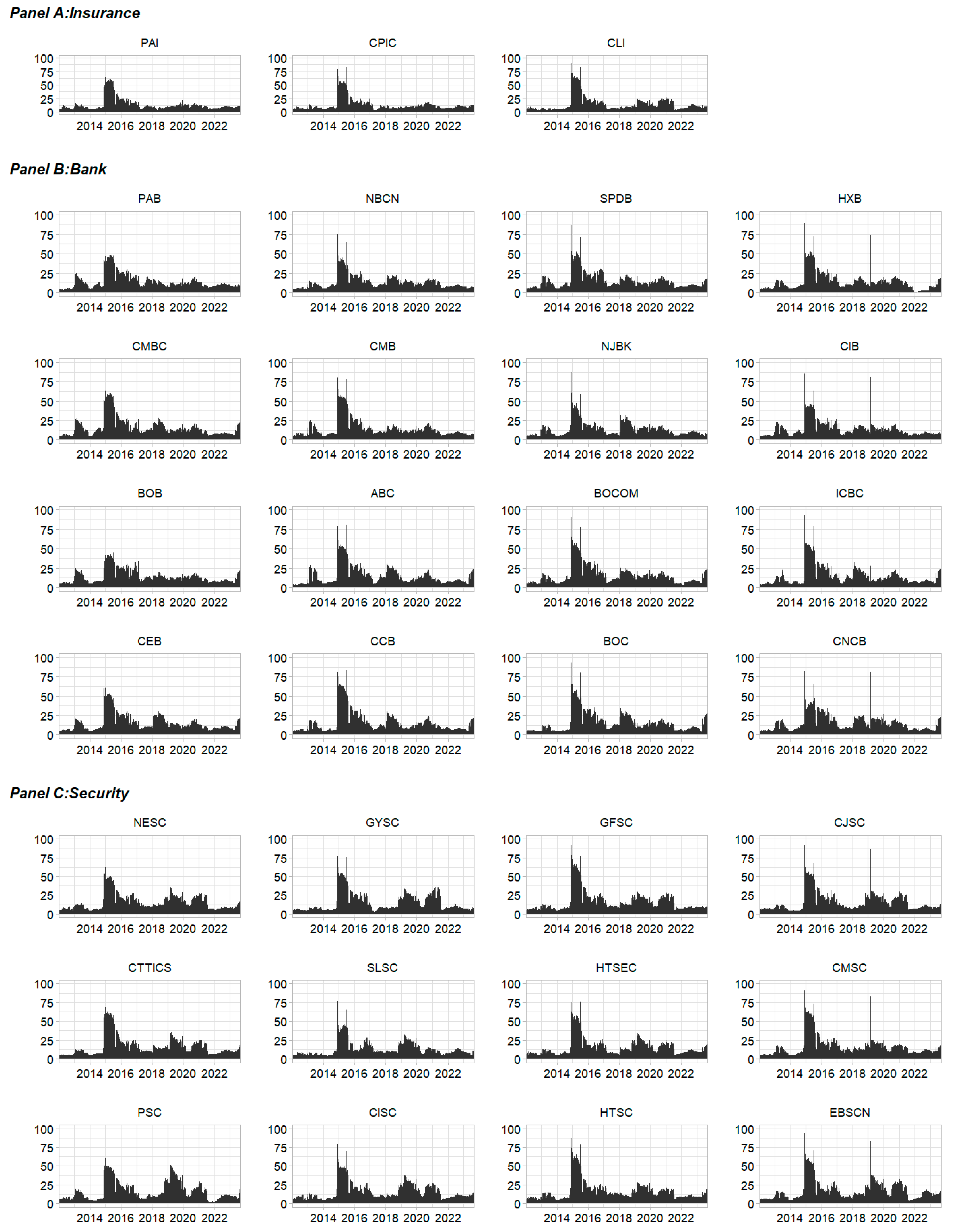
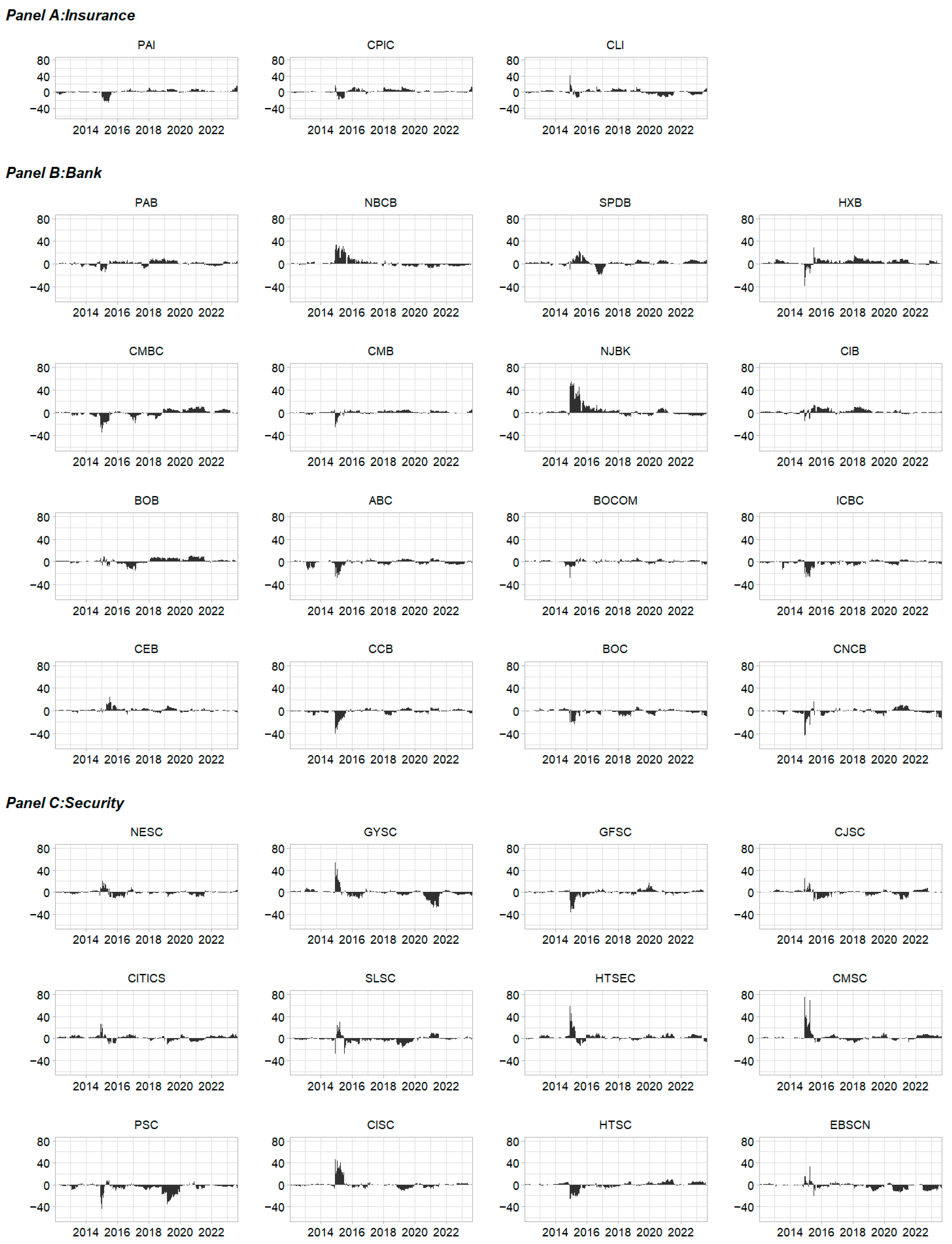
4.1.3. Institution Directional Frequency Connectedness

Next, we discuss the directional connectedness of the 31 publicly traded Chinese financial institutions. Figure 5, Figure 6 and Figure 7 illustrate each institution’s long-term dynamic from-connectedness, to-connectedness, and net-connectedness (the short- and medium-run directional connectedness is presented in Appendix A). Similar to the sectoral frequency connectedness analysis, each institution’s long-term dynamic from- and to-connectedness coincides with the total long-term connectedness. More precisely, the from-connectedness for institutions was quite similar to the dynamic long-term to-connectedness, which varied across institutions and mainly determined the dynamic long-term net-connectedness. Long-term net-connectedness varies substantially across time and institutions. Overall, a strong change was observed for all institutions in terms of long-term dynamic net-connectedness during the second cycle, which includes the bullish period and stock market crash. Six securities, including CMSC, CISC, and HTSEC, and two banks, NJBK and NBCB, were the main long-term connectedness emitters during the first half of 2015, indicating that the securities triggered the 2015 bull market before the crash. During the stock market crash, the NJBK, NBCB, and several other banks were the main long-run connectedness emitters. The four state-run commercial banks (ICBC, CCB, BOC, and ABC) were net receivers of long-term connectedness or shocks and contributed less than the other two types of commercial banks: city commercial banks.

4.2. Network Estimation Results

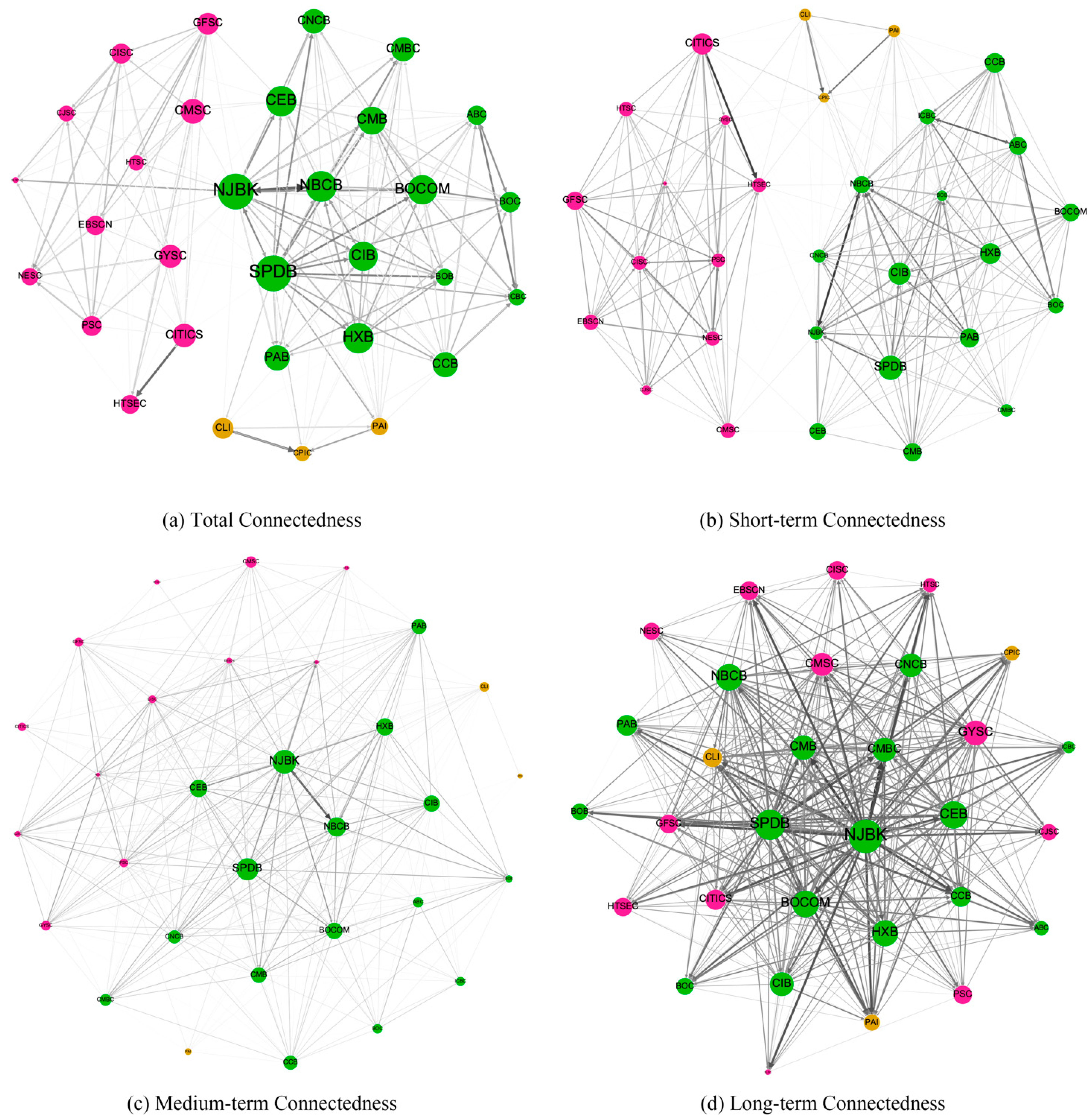
4.2.1. Full-Sample Networks

In this sub-section, an “average” network of institutions was predicted using the full sample period. Figure 8a shows the total connectedness of the network of the full sample of financial institutions. Figure 8b–d illustrate the full sample financial institution network’s short-, medium-, and long-term connectedness. Figure 8a shows that the institutions are split into three clusters, representing the three sectors. The connectedness across the three clusters is weak, as shown by the thin pairwise edges among the members of the three clusters. The results in Figure 8b–d are valid for the short-, medium-, and long-term connectedness networks, indicating that the three clusters have weak links.

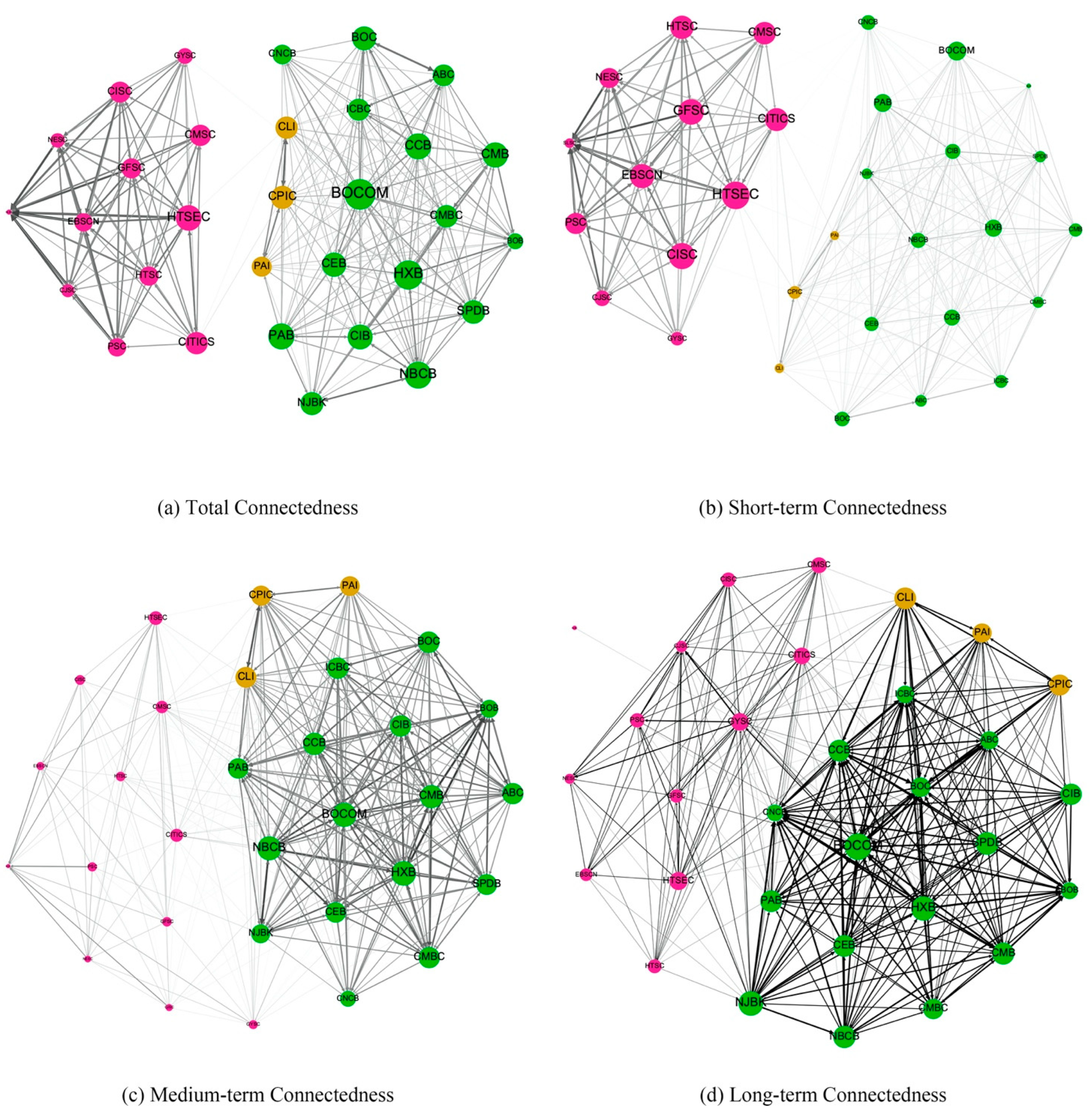
4.2.2. Network Structure on Some Critical Dates

This subsection describes the network structures corresponding to recent important dates for Chinese financial institutions. In this study, total and long-term connectedness levels reached a maximum in the second cycle, containing both the bullish period and the stock market crash. Next, a case study was conducted by investigating the connectedness network of the 31 Chinese financial institutions on 31 December 2014 (when long-term connectedness reached its maximum level during the bullish period), 30 June 2015 (the stock market crash), and 31 December 2015 (the post-crash period). Four network graphs are presented for each date: the total connectedness network and the short-, medium-, and long-term connectedness networks.

Figure 9a exhibits total connectedness as three-sector clusters but with stronger links than Figure 8a because long-term connectedness peaked during the bullish period; that is, the cluster structure becomes less robust. Figure 9b–d illustrate the connectedness network in the short-, medium-, and long-run. The full-sample analysis provided consistency between the short- and medium-run connectedness networks. In the long-run connectedness network shown in Figure 9d, the clusters of the three sectors disappear. The connectedness structure transformed from a clustered structure to a core–periphery structure, with several securities such as CMSC, CITICS, and HTSEC as core institutions. This finding coincides with the results in Section 4.1.3, providing evidence that securities triggered the 2015 Chinese bull market.

Figure 10 shows the total (frequency) connectedness network during the 2015 Chinese stock market crash (30 June 2015). Similar to Figure 8, Figure 10a–c represent the clusters of the three sectors with weak links. However, the to-connectedness of the securities and insurance sectors (node size) is smaller than that of the banking sector, indicating that securities were not risk emitters during the crash. In the long-term connectedness network in Figure 10d, the connectedness structure turns into a core–periphery structure. However, the core institutions included several banks, such as NJBK, SPDB, and CMBC, instead of securities, indicating that banks were the main risk transmitters during the crash. Worth noting is that the risk contributions of the five institutions listed in the G-SIB and G-SII lists (i.e., ICBC, BOC, CCB, ABC, and PAI) were small. One possible reason is that these systemically important institutions are well regulated. Figure 11 shows the total (frequency) connectedness network during the post-crash period, which is similar to Figure 8 and indicates the normal state.

5. Conclusions and Discussion

This study provides a new perspective on the frequency dynamics of the volatility connectedness of 31 publicly traded Chinese financial institutions (including insurers, banks, and securities). Our analysis was based on the spectral representation framework of GFEVD. First, we use volatility connectedness indices to explore the dynamic frequency characteristics of volatility connectedness pertinent to system-wide, sector-conditional, and firm-level perspectives. Next, we explored the network graphs of the frequency connectedness to gain a better understanding of the underlying network structure.

Our empirical results suggest that frequency connectedness varies in intensity and trends when a financial system experiences uncertain economic conditions or is distressed, such as during the Chinese banking liquidity crisis of 2013, the 2018–2019 Sino–U.S. Trade war, and especially the 2015–2016 Chinese stock market crash. Specifically, long-term connectedness plays an important role, peaking during periods of uncertainty. Economically, stock markets appear to crunch information swiftly and placidly during periods of short-term connectedness. This suggests that shocks are tenacious and spread over longer periods, thus affecting the market in the long-run [31] when long-term connectedness is created. The results also suggest that inter-sector connectedness is higher than cross-sector connectedness in most phases. However, cross-sector connectedness arises when economic conditions or distress are uncertain. Combining sectoral and institutional directional connectedness demonstrates that securities triggered the 2015 bull market, while banks were the fundamental risk transmitters during the stock market crash.

Overall, our studies add to the academic literature that an institution’s significance as a target or source of risks depends on the frequency and time period. The previous literature evaluated the connectedness of financial institutions only from the time domain [27,40,41,48]; it cannot explore the contribution of different frequency horizons on the overall connectedness [59]. It is important to properly measure the dynamic connectedness across time and frequency, for the connectedness generated at lower frequencies indicates that the impact is persistent and the propagation time is longer, which may lead to systemic risks more easily [30,60]. In addition, we consider the COVID-19 pandemic on the volatility connectedness of Chinese financial institutions, which is declining during the COVID-19 pandemic and rising during the COVID-19 pandemic period [61]. Our findings are inconsistent with existing research conclusions [62,63,64,65]. This is mainly due to the different financial institutions examined. The existing research has mainly examined the volatility connectedness of the banking sector, while the financial institutions in our study include banks, insurance, and securities. Institutional business connectedness is the main channel of risk contagion [30,65]. During the COVID-19 pandemic, the business connectedness among financial institutions reduced; thus, the volatility connectedness among institutions reduced due to the Chinese government’s lockdown policy [61].

Based on the above findings, we suggest that supervisory authorities should consider the connectedness indexes of dynamic time-frequency, especially by monitoring the increase in low-frequency connectedness among financial institutions in the pre-crisis period to prevent the accumulation of potential risks. In addition, supervisory authorities should pay attention to the role of different financial institutions in risk contagion and the impact of different external shocks on systemic risk and implement differentiated regulatory policies.

References

1. Xu, Q.; Zhang, Y.; Zhang, Z. Tail-risk spillovers in cryptocurrency markets. Financ. Res. Lett. 2021, 38, 101453. [Google Scholar] [CrossRef]
2. Mader, P.; Mertens, D.; Van Der Zwan, N. Financialization: An introduction. In The Routledge International Handbook of Financialization; Routledge: Oxfordshire, UK, 2020; pp. 1–16. [Google Scholar]
3. Gofman, M. Efficiency and stability of a financial architecture with too-interconnected-to-fail institutions. J. Financ. Econ. 2017, 124, 113–146. [Google Scholar] [CrossRef]
4. Barucca, P.; Bardoscia, M.; Caccioli, F.; D’Errico, M.; Visentin, G.; Caldarelli, G.; Battiston, S. Network valuation in financial systems. Math. Financ. 2020, 30, 1181–1204. [Google Scholar] [CrossRef]
5. Duarte, F.; Eisenbach, T.M. Fire-sale spillovers and systemic risk. J. Financ. 2021, 76, 1251–1294. [Google Scholar] [CrossRef]
6. Fang, L.; Sun, B.; Li, H.; Yu, H. Systemic risk network of Chinese financial institutions. Emerg. Mark. Rev. 2018, 35, 190–206. [Google Scholar] [CrossRef]
7. Li, J.; Yao, Y.; Li, J.; Zhu, X. Network-based estimation of systematic and idiosyncratic contagion: The case of Chinese financial institutions. Emerg. Mark. Rev. 2019, 40, 100624. [Google Scholar] [CrossRef]
8. Alessandri, P.; Masciantonio, S.; Zaghini, A. Tracking Banks’ Systemic Importance Before and After the Crisis. Int. Financ. 2015, 18, 157–186. [Google Scholar] [CrossRef]
9. Diebold, F.X.; Yilmaz, K. Measuring financial asset return and volatility spillovers, with application to global equity markets. Econ. J. 2009, 119, 158–171. [Google Scholar] [CrossRef]
10. Bahloul, S.; Khemakhem, I. Dynamic return and volatility connectedness between commodities and Islamic stock market indices. Resour. Policy 2021, 71, 101993. [Google Scholar] [CrossRef]
11. Youssef, M.; Mokni, K.; Ajmi, A.N. Dynamic connectedness between stock markets in the presence of the COVID-19 pandemic: Does economic policy uncertainty matter? Financ. Innov. 2021, 7, 13. [Google Scholar] [CrossRef]
12. Umar, Z.; Jareño, F.; Escribano, A. Agricultural commodity markets and oil prices: An analysis of the dynamic return and volatility connectedness. Resour. Policy 2021, 73, 102147. [Google Scholar] [CrossRef]
13. Gong, X.; Xu, J. Geopolitical risk and dynamic connectedness between commodity markets. Energy Econ. 2022, 110, 106028. [Google Scholar] [CrossRef]
14. Chen, R.; Iqbal, N.; Irfan, M.; Shahzad, F.; Fareed, Z. Does financial stress wreak havoc on banking, insurance, oil, and gold markets? New empirics from the extended joint connectedness of TVP-VAR model. Resour. Policy 2022, 77, 102718. [Google Scholar] [CrossRef]
15. Arfaoui, N.; Yousaf, I.; Jareño, F. Return and volatility connectedness between gold and energy markets: Evidence from the pre-and post-COVID vaccination phases. Econ. Anal. Policy 2023, 77, 617–634. [Google Scholar] [CrossRef]
16. Bostanci, G.; Yilmaz, K. How connected is the global sovereign credit risk network? J. Bank. Financ. 2020, 113, 105761. [Google Scholar] [CrossRef]
17. Yang, L.; Hamori, S. Modeling the global sovereign credit network under climate change. Int. Rev. Financ. Anal. 2023, 87, 102618. [Google Scholar] [CrossRef]
18. Hung, N.T.; Nguyen, L.T.M.; Vo, X.V. Exchange rate volatility connectedness during COVID-19 outbreak: DECO-GARCH and Transfer Entropy approaches. J. Int. Financ. Mark. Inst. Money 2022, 81, 101628. [Google Scholar] [CrossRef]
19. Huynh, T.L.D.; Nasir, M.A.; Nguyen, D.K. Spillovers and connectedness in foreign exchange markets: The role of trade policy uncertainty. Q. Rev. Econ. Financ. 2020, 87, 191–199. [Google Scholar] [CrossRef]
20. Wen, T.; Wang, G.J. Volatility connectedness in global foreign exchange markets. J. Multinatl. Financ. Manag. 2020, 54, 100617. [Google Scholar] [CrossRef]
21. Koutmos, D. Return and volatility spillovers among cryptocurrencies. Econ. Lett. 2018, 173, 122–127. [Google Scholar] [CrossRef]
22. Hasan, M.; Naeem, M.A.; Arif, M.; Yarovaya, L. Higher moment connectedness in cryptocurrency market. J. Behav. Exp. Financ. 2021, 32, 100562. [Google Scholar] [CrossRef]
23. Li, Z.; Mo, B.; Nie, H. Time and frequency dynamic connectedness between cryptocurrencies and financial assets in China. Int. Rev. Econ. Financ. 2023, 86, 46–57. [Google Scholar] [CrossRef]
24. Mensi, W.; Al Rababa’a, A.R.; Vo, X.V.; Kang, S.H. Asymmetric spillover and network connectedness between crude oil, gold, and Chinese sector stock markets. Energy Econ. 2021, 98, 105262. [Google Scholar] [CrossRef]
25. Dai, Z.; Zhu, H.; Zhang, X. Dynamic spillover effects and portfolio strategies between crude oil, gold and Chinese stock markets related to new energy vehicle. Energy Econ. 2022, 109, 105959. [Google Scholar] [CrossRef]
26. Härdle, W.K.; Wang, W.; Yu, L. TENET: Tail-Event driven NETwork risk. J. Econom. 2016, 192, 499–513. [Google Scholar] [CrossRef]
27. Wang, G.J.; Jiang, Z.Q.; Lin, M.; Xie, C.; Stanley, H.E. Interconnectedness and systemic risk of China’s financial institutions. Emerg. Mark. Rev. 2018, 35, 1–18. [Google Scholar] [CrossRef]
28. Wang, G.J.; Xie, C.; Zhao, L.; Jiang, Z.Q. Volatility connectedness in the Chinese banking system: Do state-owned commercial banks contribute more? J. Int. Financ. Mark. Inst. Money 2018, 57, 205–230. [Google Scholar] [CrossRef]
29. Diebold, F.X.; Yilmaz, K. On the network topology of variance decompositions: Measuring the connectedness of financial firms. J. Econom. 2014, 182, 119–134. [Google Scholar] [CrossRef]
30. Liang, Q.; Lu, Y.; Li, Z. Business connectedness or market risk? Evidence from financial institutions in China. China Econ. Rev. 2020, 62, 101503. [Google Scholar] [CrossRef]
31. Baruník, J.; Křehlík, T. Measuring the Frequency Dynamics of Financial Connectedness and Systemic Risk. J. Financ. Econom. 2018, 16, 271–296. [Google Scholar] [CrossRef]
32. Bissoondoyal-Bheenick, E.; Do, H.; Hu, X.; Zhong, A. Learning from SARS: Return and volatility connectedness in COVID-19. Financ. Res. Lett. 2021, 41, 101796. [Google Scholar] [CrossRef]
33. Elnahass, M.; Trinh, V.Q.; Li, T. Global banking stability in the shadow of Covid-19 outbreak. J. Int. Financ. Mark. Inst. Money 2021, 72, 101322. [Google Scholar] [CrossRef]
34. Wang, Y.; Zhang, D.; Wang, X.; Fu, Q. How does COVID-19 affect China’s insurance market? Emerg. Mark. Financ. Trade 2020, 56, 2350–2362. [Google Scholar] [CrossRef]
35. Sun, Y.; Wu, M.; Zeng, X.; Peng, Z. The impact of COVID-19 on the Chinese stock market: Sentimental or substantial? Financ. Res. Lett. 2021, 38, 101838. [Google Scholar] [CrossRef] [PubMed]
36. Cheng, T.; Liu, J.; Yao, W.; Zhao, A.B. The impact of COVID-19 pandemic on the volatility connectedness network of global stock market. Pac. Basin Financ. J. 2022, 71, 101678. [Google Scholar] [CrossRef]
37. Umar, Z.; Jareño, F.; Escribano, A. Dynamic return and volatility connectedness for dominant agricultural commodity markets during the COVID-19 pandemic era. Appl. Econ. 2022, 54, 1030–1054. [Google Scholar] [CrossRef]
38. Umar, Z.; Jareño, F.; de la O González, M. The impact of COVID-19-related media coverage on the return and volatility connectedness of cryptocurrencies and fiat currencies. Technol. Forecast. Soc. Chang. 2021, 172, 121025. [Google Scholar] [CrossRef]
39. Hamouda, F. What can we learn about repurchase programmes and systemic risk? Evidence from US banks during financial turmoil. J. Risk Manag. Financ. Inst. 2023, 16, 34–51. [Google Scholar]
40. Diebold, F.X.; Yilmaz, K. Trans-Atlantic equity volatility connectedness: US and European financial institutions, 2004–2014. J. Financ. Econom. 2015, 14, 81–127. [Google Scholar]
41. Shahzad, U.; Ferraz, D.; Nguyen, H.H.; Cui, L. Investigating the spill overs and connectedness between financial globalization, high-tech industries and environmental footprints: Fresh evidence in context of China. Technol. Forecast. Soc. Change 2022, 174, 121205. [Google Scholar] [CrossRef]
42. Jiang, J.; Piljak, V.; Tiwari, A.K.; Äijö, J. Frequency volatility connectedness across different industries in China. Financ. Res. Lett. 2019, 101376. [Google Scholar] [CrossRef]
43. Tiwari, A.K.; Cunado, J.; Gupta, R.; Wohar, M.E. Volatility spillovers across global asset classes: Evidence from time and frequency domains. Q. Rev. Econ. Financ. 2018, 70, 194–202. [Google Scholar] [CrossRef]
44. Wang, X.; Wang, Y. Volatility spillovers between crude oil and Chinese sectoral equity markets: Evidence from a frequency dynamics perspective. Energy Econ. 2019, 80, 995–1009. [Google Scholar] [CrossRef]
45. Diebold, F.X.; Yilmaz, K. Better to give than to receive: Predictive directional measurement of volatility spillovers. Int. J. Forecast. 2012, 28, 57–66. [Google Scholar] [CrossRef]
46. Baruńik, J.; Kočenda, E.; Vácha, L.S. Volatility spillovers across petroleum markets. Energy J. 2015, 36, 309–329. [Google Scholar] [CrossRef]
47. Adekoya, O.B.; Oliyide, J.A.; Noman, A. The volatility connectedness of the EU carbon market with commodity and financial markets in time-and frequency-domain: The role of the US economic policy uncertainty. Resour. Policy 2021, 74, 102252. [Google Scholar] [CrossRef]
48. Barigozzi, M.; Brownlees, C. Nets: Network estimation for time series. J. Appl. Econom. 2019, 34, 347–364. [Google Scholar] [CrossRef]
49. Jiang, S.; Li, Y.; Lu, Q.; Wang, S.; Wei, Y. Volatility communicator or receiver? Investigating volatility spillover mechanisms among Bitcoin and other financial markets. Res. Int. Bus. Financ. 2022, 59, 101543. [Google Scholar] [CrossRef]
50. Koop, G.; Pesaran, M.H.; Potter, S.M. Impulse response analysis in nonlinear multivariate models. J. Econom. 1996, 74, 119–147. [Google Scholar] [CrossRef]
51. Pesaran, H.H.; Shin, Y. Generalized impulse response analysis in linear multivariate models. Econ. Lett. 1998, 58, 17–29. [Google Scholar] [CrossRef]
52. Stiassny, A. A spectral decomposition for structural VAR models. Empir. Econ. 1996, 21, 535–555. [Google Scholar] [CrossRef]
53. Nicholson, W.B.; Matteson, D.S.; Bien, J. VARX-L: Structured regularization for large vector autoregressions with exogenous variables. Int. J. Forecast. 2017, 33, 627–651. [Google Scholar] [CrossRef]
54. Simon, N.; Friedman, J.; Hastie, T.; Tibshirani, R. A sparse-group lasso. J. Comput. Graph. Stat. 2013, 22, 231–245. [Google Scholar] [CrossRef]
55. Dew-Becker, I.; Giglio, S. Asset pricing in the frequency domain: Theory and empirics. Rev. Financ. Stud. 2016, 29, 2029–2068. [Google Scholar] [CrossRef]
56. Demirer, M.; Diebold, F.X.; Liu, L.; Yilmaz, K. Estimating global bank network connectedness. J. Appl. Econom. 2018, 33, 1–15. [Google Scholar] [CrossRef]
57. Jacomy, M.; Venturini, T.; Heymann, S.; Bastian, M. ForceAtlas2, a continuous graph layout algorithm for handy network visualization designed for the Gephi software. PLoS ONE 2014, 9, e98679. [Google Scholar] [CrossRef]
58. Garman, M.B.; Klass, M.J. On the Estimation of Security Price Volatilities from Historical Data. J. Bus. 1980, 53, 67–78. [Google Scholar] [CrossRef]
59. Shah, A.A.; Paul, M.; Bhanja, N.; Dar, A.B. Dynamics of connectedness across crude oil, precious metals and exchange rate: Evidence from time and frequency domains. Resour. Policy 2021, 73, 102154. [Google Scholar] [CrossRef]
60. Wang, Y.; Zhang, Z.; Li, X.; Chen, X.; Wei, Y. Dynamic return connectedness across global commodity futures markets: Evidence from time and frequency domains. Phys. A Stat. Mech. Its Appl. 2020, 542, 123464. [Google Scholar] [CrossRef]
61. Ouyang, Z.; Zhou, X.; Xie, N. Time-varying connectedness measurement of Chinese financial institutions: New evidence from the frequency domain perspective. Syst. Eng. Theory Pract. 2022, 42, 2087–2101. [Google Scholar] [CrossRef]
62. Foglia, M.; Addi, A.; Angelini, E. The Eurozone banking sector in the time of COVID-19: Measuring volatility connectedness. Glob. Financ. J. 2022, 51, 100677. [Google Scholar] [CrossRef]
63. Chen, Y.P.; Chen, Y.L.; Chiang, S.H.; Mo, W.S. Determinants of connectedness in financial institutions: Evidence from Taiwan. Emerg. Mark. Rev. 2023, 55, 100951. [Google Scholar] [CrossRef]
64. Costa, A.; Matos, P.; da Silva, C. Sectoral connectedness: New evidence from US stock market during COVID-19 pandemics. Financ. Res. Lett. 2022, 45, 102124. [Google Scholar] [CrossRef] [PubMed]
65. Fan, X.; Wang, Y.; Wang, D. Network connectedness and China’s systemic financial risk contagion—An analysis based on big data. Pac. Basin Financ. J. 2021, 68, 101322. [Google Scholar] [CrossRef]
Figure 1. The total volatility connectedness ( T C ), which is computed using Diebold and Yilmaz (2014) measure on moving window with a length of 250 days, VARs using the lag group LASSO with the max lag order p = 5 and the predictive horizon H = 100 days were estimated.
Systems 11 00502 g001
Figure 2. The total volatility connectedness at frequency band d ( T C d ) with d 1 1 , 5   i n   b l u e ,   d 2 5 , 20   g r e e n ,   d 3 20 , 100   r e d , computed using Baruník and Křehlík (2018) measure on moving window with a length of 250 days, VARs using the lag group LASSO with the max lag order p = 5 .
Systems 11 00502 g002
Figure 3. Sector directional connectedness. Show the connectedness within the sector (Within-Connectedness), directional connectedness from other sectors (From-Connectedness), directional connectedness to other sectors (To-Connectedness), and the net directional connectedness (To-Connectedness minus From-Connectedness).
Systems 11 00502 g003
Figure 4. Frequency decomposition of sector directional connectedness with d 1 1 , 5 ,   d 2 5 , 20 ,   d 3 20 , 100 .
Systems 11 00502 g004
Figure 5. Long-term from-connectedness for 31 Chinese publicly traded financial institutions.
Systems 11 00502 g005
Figure 6. Long-term to-connectedness for 31 Chinese publicly traded financial institutions.
Systems 11 00502 g006
Figure 7. Long-term net-connectedness for 31 Chinese publicly traded financial institutions.
Systems 11 00502 g007
Figure 8. Full sample connectedness network for 31 Chinese publicly traded financial institutions, 2011–2019. Created by open-source software Gephi, the nodes’ position is determined by the ForceAtlas2 algorithm. The node sector is indicated by the node color: green, red, and yellow indicate banks, securities, and insurers, respectively. Only the top 50% of the edges are visible for better visualization.
Systems 11 00502 g008
Figure 9. Connectedness network for 31 Chinese publicly traded financial institutions on 31 December 2014 (50% of the edges visible). Created by open-source software Gephi, the nodes’ position is determined by the ForceAtlas2 algorithm. The node sector is indicated by the node color: green, red, and yellow indicate banks, securities, and insurers, respectively. Only the top 50% of the edges are visible for better visualization.
Systems 11 00502 g009
Figure 10. Connectedness network for 31 Chinese publicly traded financial institutions on 30 June 2015 (50% of the edges visible). Created by open-source software Gephi, the nodes’ position is determined by the ForceAtlas2 algorithm. The node sector is indicated by the node color: green, red, and yellow indicate banks, securities, and insurers, respectively. Only the top 50% of the edges are visible for better visualization.
Systems 11 00502 g010
Figure 11. Connectedness network for 31 Chinese publicly traded financial institutions on 31 December 2015 (50% of the edges visible). Created by open-source software Gephi, the nodes’ position is determined by the ForceAtlas2 algorithm. The node sector is indicated by the node color: green, red, and yellow indicate banks, securities, and insurers, respectively. Only the top 50% of the edges are visible for better visualization.
Systems 11 00502 g011