Bayesian Inference of System Reliability for Multicomponent Stress-Strength Model under Marshall-Olkin Weibull Distribution

Abstract

Industrial systems often have redundant structures for improving reliability and avoiding sudden failures, and a parallel system is one of the special redundant systems. In this paper, we consider the problem of reliability estimation for a parallel system when one stress variable is involved, which is called the multicomponent stress-strength model. The parallel system contains two components, and their joint lifetime follows a Marshall–Olkin bivariate Weibull distribution, while the stress variable is assumed to be the Weibull distribution. Due to the complicated form of the likelihood function, a data augmentation method is proposed, and then the Gibbs sampling algorithm is constructed to obtain the Bayesian estimation of the system reliability. The proposed method is evaluated by a simulated dataset and Monte Carlo simulation study. The simulation results show that the proposed method performs well in terms of relative bias, mean squared error and frequentist coverage probability.

1. Introduction

Modern industrial systems are often designed with high-quality standards. A redundant structure is a way to improve system reliability. For example, a cloud storage server usually has at least one backup to help customers keep valuable information and data sets safe; a commercial aircraft has a spare engine to deal with sudden failures. Parallel structure as a special redundant structure has been widely adopted in many industrial products, for instance, power generation systems, production systems, pump systems, etc. When systems are delivered to be used in practice, there exist some factors to affect the reliability of systems such as operating environments, external shocks and operators. These factors can be viewed as stresses that the system experiences during functioning. In this case, the reliability of the parallel system is usually assessed through stress-strength model [1]. The stress-strength model is one of the most widely used reliability models, which was first introduced by Birnbaum and McCarty [2]. In this model, a system fails if its stress exceeds its strength. Therefore, the reliability of the system is defined as the probability that the strength of the system exceeds its stress: $R=P(Y>X)$, where X denotes the stress variable and Y represents the strength of the system. The stress-strength model has been systematically studied when Y is the lifetime of a component. A comprehensive review on this area can be found in Kotz et al. [3], and the references therein.

In recent years, many studies have been focused on estimating the reliability under the stress-strength model through various statistical methods. For example, Wang et al. [4] developed a generalized inference procedure for the generalized exponential stress-strength model. When the stress and strength variables are generalized exponential distributed with a common rate parameter, the generalized confidence interval of the reliability of the stress-strength model is derived. In addition, based on the Fisher’s Z transformation, a modified generalized confidence interval for the reliability of the stress-strength model with unequal rate parameters is proposed. Ghitany et al. [5] gave the point and interval estimation of the reliability R of the stress strength model under the power Lindley distribution based on the maximum likelihood (ML), nonparametric, and parameter bootstrap methods. Jose [6] assumed that the stress and strength components are distributed with discrete phases, and estimated the reliability of the stress-strength model of single component and multicomponent systems. The reliability expression of the stress-strength model based on the matrix is derived, and the reliability is estimated by the ML method through an EM algorithm. In addition to using classical statistical inference methods, Bayesian methods are also widely used to infer the reliability of stress strength models. See [7,8,9]. In addition, to compare the estimation performance of the classical method and Bayesian method on the reliability of the stress-strength model, many studies often use both the frequency analysis method and Bayesian method to estimate the reliability at the same time. See [10,11,12,13].

Since the classical stress-strength model only involves one strength variable, for modern products with complicated structures, it is too limited to assess the reliability of a system involving multiple strength components. In this regard, some scholars began to study the multicomponent stress-strength model. The multicomponent stress-strength model was first proposed by Bhattacharyya and Johnson [14], in which it is assumed that the system is a k-out-of-n system with common distributed components. That is, the system has n independent strength components, the lifetime of which follow the same distribution. When more than k of the n components fail, the system will fail. Subsequently, based on the research of Bhattacharyya and Johnson [14], the studies on the multicomponent stress-strength model have been extended to other types of systems, where the strength of each component follows different lifetime distributions. For example, Kumaraswamy distribution (Dey et al. [15]), generalized half-logistic distribution (Liu et al. [16]), Gompertz distribution (Jha et al. [17]), generalized logistic distribution (Rasekhi et al. [18]), etc. In addition, Wang et al. [19] estimated the reliability of the multicomponent stress-strength model based on Kumaraswamy distribution by the ML method, and proposed a generalized inference to obtain the point and interval estimates of R. Kang et al. [20] estimated the reliability of the multicomponent stress-strength model under exponential distribution using objective Bayesian methods. However, most of the existing studies in this field assume that the strength variables are independent of each other, which may not be true in practice. The strength components from the same system are usually correlated, because they function in the same environments (Luo et al. [21]). Two ways are usually utilized to describe correlations among the random variables: multivariate lifetime distributions (Kzlaslan and Nadar [22], Kundu and Dey [23]), and copula functions (Bai et al. [24]). Then, statistical inference of the reliability for the multicomponent stress-strength model is implemented when the correlations are considered by [25,26,27]. However, the above studies are based on the assumption that the strength variables are from a series system. To the best of our knowledge, the studies on parallel systems under the multicomponent stress-strength model are rare. Therefore, this paper will study the reliability of the multicomponent stress-strength model involving one stress and two correlated strength components from the parallel system based on the Marshall–Olkin bivariate Weibull (MOBW) distribution. Our paper differs from Kundu and Gupta [23] in two aspects. Firstly, the model considered in this paper has one more stress variable compared with Kundu and Gupta [23], which can be viewed as an external factor that affects the reliability of the parallel system. Thus, the emphasis of this paper is to estimate the reliability of the parallel system. The other difference lies in the method of estimating the model parameters. Kundu and Gupta [23] proposed an importance sampling algorithm to estimate the model parameters. We use the data augmentation method to simplify the original likelihood function, and obtain the Bayesian estimate of R by Gibbs sampling. Although the importance sampling algorithm is efficient, as stated by Kundu and Gupta [23], the instrumental distribution used in importance sampling will be much more complicated in our model because it includes more parameters, which is not an easy way to figure out. Although the data augmentation method has been mentioned in Ghosh et al. [28], the detailed implementation of this method depends on the specific model, and the key point is to find some latent variables that can be used to simplify the likelihood function. Kundu and Nekoukhou [29] have used the data augmentation method and Gibbs sampling to obtain the parameter estimation of bivariate discrete Weibull distribution. However, the random variables involved in this paper are continuous, and the model is also much different. Overall, the contribution of this paper has two aspects. Firstly, the correlation between strength components from the parallel system are considered, which is reasonable and consistent with the practical situation. Then, a data augmentation procedure is proposed for simplifying likelihood function, which greatly alleviates the difficulty of statistical inference.

The paper is organized as follows. In Section 2, we introduce the multicomponent stress-strength model. The data augmentation method is proposed to simplify the likelihood function in Section 3. Section 4 is devoted to the Markov chain Monte Carlo (MCMC) algorithm for obtaining Bayesian estimation of reliability. Simulation studies are performed for assessing the proposed method in terms of relative error, mean squared error and frequentist coverage probability in Section 5. An artificial dataset is also analyzed for illustration in Section 5. Finally, we give a conclusion for this paper in Section 6.

2. Model

2.1. MOBW Distribution

Marshall and Olkin [30] proposed the MOBW distribution, which was described as follows. Assume that $U_1,U_2,U_3$ are the three independent random variables, and 

$$U_1\sim Weibull(\beta ,{\lambda }_1),U_2\sim Weibull(\beta ,{\lambda }_2),U_3\sim Weibull(\beta ,{\lambda }_3),$$

(1)

where $Weibull(\beta ,\lambda )$ represents the Weibull distribution with the shape parameter of $\beta$, and the scale parameter of $\lambda$. Its probability density function (PDF) is formulated as

$$\begin{array}{cc}\hfill f_W\left(x\right|\beta ,\lambda )& =\beta \lambda x^{\beta -1}exp(-\lambda x^{\beta }),x>0,\lambda >0,\beta >0.\hfill \end{array}$$

Therefore, its cumulative distribution function (CDF) and survival function (SF) are as follows:

$$\begin{array}{cc}\hfill F_W\left(x\right|\beta ,\lambda )& =1-exp(-\lambda x^{\beta }),\hfill \\ \hfill S_W\left(x\right|\beta ,\lambda )& =exp(-\lambda x^{\beta }).\hfill \end{array}$$

Further, we define the variables

$$X=min(U_1,U_3)\mathrm{and}Y=min(U_2,U_3).$$

(2)

Then, $(X,Y)$ follows MOBW distribution with the parameters $(\beta ,{\lambda }_1,{\lambda }_2,{\lambda }_3)$, and we denote it as $MOBW(\beta ,{\lambda }_1,{\lambda }_2,{\lambda }_3)$. Therefore, the joint SF of $(X,Y)$ is

$$\begin{array}{c}\hfill S_{X,Y}(x,y)=P(X>x,Y>y)=exp\left(-{\lambda }_1{x}^{\beta }-{\lambda }_2{y}^{\beta }-{\lambda }_3{\left(max(x,y)\right)}^{\beta }\right),x,y>0,\end{array}$$

and the joint PDF of $(X,Y)$ is

$$f_{X,Y}(x,y)=\left\{\begin{array}{c}{\lambda }_2({\lambda }_1+{\lambda }_3){\beta }^2{\left(xy\right)}^{\beta -1}exp(-({\lambda }_1+{\lambda }_3)x^{\beta }-{\lambda }_2{y}^{\beta }),x>y\hfill \\ {\lambda }_1({\lambda }_2+{\lambda }_3){\beta }^2{\left(xy\right)}^{\beta -1}exp(-({\lambda }_2+{\lambda }_3)y^{\beta }-{\lambda }_1{x}^{\beta }),x<y\hfill \\ {\lambda }_3\beta x^{\beta -1}exp(-\lambda x^{\beta }),x=y,\hfill \end{array}\right.,$$

(3)

where $\lambda ={\lambda }_1+{\lambda }_2+{\lambda }_3$. Since the shape parameters of the random variable $U_1,U_2$ and $U_3$ are the same, the marginal distributions of X and Y are still from the Weibull family. That is, $X\sim Weibull(\beta ,{\lambda }_1^{*})$, and  $Y\sim Weibull(\beta ,{\lambda }_2^{*})$, where ${\lambda }_1^{*}={\lambda }_1+{\lambda }_3,{\lambda }_2^{*}={\lambda }_2+{\lambda }_3$. In addition, $min(X,Y)\sim Weibull(\beta ,\lambda )$. When $\beta =1$, MOBW distribution degenerates to the Marshall–Olkin bivariate exponential distribution with parameters $({\lambda }_1,{\lambda }_2,{\lambda }_3)$. When ${\lambda }_3=0$, the random variables X and Y are independent with each other. If ${\lambda }_3>0$, then the random variables X and Y are correlated. Therefore, ${\lambda }_3$ can be viewed as the control parameter of the correlation between random variables X and Y. Moreover, according to the PDF of MOBW distribution (3), it is known that the MOBW distribution has a continuous part and a singular part. More discussions about MOBW distribution can be found in Kundu and Dey [31].

2.2. Multicomponent Stress-Strength Model

Now, we consider a system composed of two strength components in parallel. Assume that X and Y are the two strength random variables from the parallel system, and that T is the stress random variable. In addition, T and $(X,Y)$ are assumed to be independent of each other, but the strength variables X and Y are correlated. We assume $(X,Y)\sim MOBW((\beta ,{\lambda }_1,{\lambda }_2,{\lambda }_3)$, and the stress variable $T\sim Weibull(\beta ,\theta )$. Let $Z=max(X,Y)$. Then, Z denotes the lifetime or strength of the parallel system. The PDF of Z can be derived and formulated as

$$\begin{array}{cc}\hfill f_Z\left(z\right)& =({\lambda }_1+{\lambda }_3)\beta z^{\beta -1}exp\left(({\lambda }_1+{\lambda }_3)z^{\beta }\right)+({\lambda }_2+{\lambda }_3)\beta z^{\beta -1}exp\left(({\lambda }_2+{\lambda }_3)z^{\beta }\right)\hfill \\ \hfill & -\lambda \beta z^{\beta -1}exp\left(\lambda z^{\beta }\right).\hfill \end{array}$$

(4)

Then, the reliability of parallel system can be defined as $R=P(T<Z)$, which can be expressed as:

$$\begin{array}{cc}\hfill R& =P(T<Z)=\frac{\theta }{{\lambda }_1+{\lambda }_3+\theta }+\frac{\theta }{{\lambda }_2+{\lambda }_3+\theta }-\frac{\theta }{\lambda +\theta }.\hfill \end{array}$$

(5)

Assume that there are n parallel systems tested in an experiment. The observed failure time of the systems are $(z_1,\dots ,z_n)$, and their corresponding stresses are $(t_1,\dots ,t_n)$. Then, based on the observed data $\{z_1,\dots ,z_n,t_1,\dots ,t_n\}$, the likelihood function of the model parameters $\Omega =(\beta ,\theta ,{\lambda }_1,{\lambda }_2,{\lambda }_3)$ is

$$\begin{array}{cc}\hfill L(\Omega |z_1,\dots ,z_n,t_1,\dots ,t_n)& =\prod _i^n\beta \theta t_i^{\beta -1}exp(-\theta t_i^{\beta })\left[({\lambda }_1+{\lambda }_3)\beta z_i^{\beta -1}exp(({\lambda }_1+{\lambda }_3)z_i^{\beta })\right.\hfill \\ \hfill & \left.+({\lambda }_2+{\lambda }_3)\beta z_i^{\beta -1}exp(({\lambda }_2+{\lambda }_3)z_i^{\beta })-\lambda \beta z_i^{\beta -1}exp(\lambda z_i^{\beta })\right].\hfill \end{array}$$

(6)

The ML estimator of $\Omega$ can be obtained by maximizing $logL(\Omega |z_1,...,z_n,t_1,...,t_n)$. However, direct optimization can hardly get satisfactory results, because the optimization is very sensitive to the initial values. Notice that the failure time of parallel system is the maximum between the realizations of X and Y, and only the maximum one can be observed. Thus, $\{z_1,\dots ,z_n\}$ are a class of data with missing partial information, and the complete data should be $\{(x_i,y_i),i=1,\dots ,n\}$, where $x_i$ and $y_i$ are the failure time of the first and second components. In the Bayesian framework, the missing information can be treated as latent variables, and can be included in the MCMC algorithm for posterior sampling. This is the basis for the data augmentation method that will be proposed in the next section.

3. Data Augmentation

For better understanding the spirit of the data augmentation method for the proposed stress-strength model, we assume that the information of which component failed first is also known. That is, the observed data of parallel systems are $\{(z_i,E_i),i=1,\dots ,n\}$, where $E_i$ is the failure index of the i-th system, e.g., $E_i=1$ denotes $x_i>y_i$; $E_i=2$ represents $x_i<y_i$; $E_i=0$ means $x_i=y_i$. Define $V_1=\{i:E_i=1\}$, $V_2=\{i:E_i=2\}$, and $V_3=\{i:E_i=0\}$. Let $n_1=\left|V_1\right|$, $n_2=\left|V_2\right|$ and $n_3=\left|V_3\right|$, where $|V_j|$, $j=1,2,3$, denotes the number of elements in the set $V_j$, and $n=n_1+n_2+n_3$. Then, the data can be divided into three parts: $D_1=\{z_i:i\in V_1\}$, $D_2=\{z_i:i\in V_2\}$, and $D_3=\{z_i:i\in V_3\}$. Although the data information of $D_1$, $D_2$ and $D_3$ are incomplete, some potential information can be found in these subsets. For example, for $D_1$, we know that $z_i=max\{x_i,y_i\}=x_i$. $y_i$ is unobservable in this case. If we treat $y_i$ as a latent variable, then its support will be $(0,x_i)$, and its PDF is

$$f_{Y_i}\left(y\right|\beta ,{\lambda }_2,{\lambda }_3,x_i)=\frac{1}{{\int }_0^{x_i}{f}_W(y;\beta ,{\lambda }_2+{\lambda }_3)\mathrm{d}y}{f}_W(y;\beta ,{\lambda }_2+{\lambda }_3),0<y<x_i.$$

(7)

Similarly, if $z_i\in D_2$, then $z_i=max\{x_i,y_i\}=y_i$, and $x_i$ is unobservable. In this case, the PDF of $x_i$ is

$$f_{X_i}\left(x\right|\beta ,{\lambda }_1,{\lambda }_3,y_i)=\frac{1}{{\int }_0^{y_i}{f}_W(x;\beta ,{\lambda }_1+{\lambda }_3)\mathrm{d}x}{f}_W(x;\beta ,{\lambda }_1+{\lambda }_3),0<x<y_i.$$

(8)

Therefore, we know that the complete data for $D_1$, $D_2$ and $D_3$ should be $I_1=\{(x_{1i},y_{1i}),i=1,...,n_1\}$, $I_2=\{(x_{2i},y_{2i}),i=1,...,n_2\}$, and $I_3=\{z_i,i=1,...,n_3\}$, respectively, where the observed data are $(x_{11},\dots ,x_{1n_1},$$y_{21},\dots ,y_{2n_2},z_1,\dots ,z_{n_3})$ and the unobserved data are $(y_{11},\dots ,y_{1n_1},x_{21},\dots ,x_{2n_2})$.

According to the definition of MOBW distribution, $(x_i,y_i)$ can be further augmented through the three underling Weibull distributions (1). That is, for each $(x_i,y_i)$, there exists a set of underlying Weibull distributed realizations $(u_{1i},u_{2i},u_{3i})$. When $(x_{1i},y_{1i})\in I_1$, then from the definition (2), we know that there are two relationships between $u_{1i},u_{2i}$ and $u_{3i}$. That is, $u_{2i}<u_{3i}<u_{1i}$ or $u_{2i}<u_{1i}<u_{3i}$. Then, for this case, we define a binary random variable $P_i$:

$$P_i=\left\{\begin{array}{c}0,u_{2i}<u_{3i}<u_{1i},\hfill \\ 1,u_{2i}<u_{1i}<u_{3i}.\hfill \end{array}\right.$$

It can be easily shown that $P(P_i=1)=\frac{{\lambda }_1}{{\lambda }_1+{\lambda }_3}$. Thus, $P_i$ follows Bernoulli distribution with success probability $\frac{{\lambda }_1}{{\lambda }_1+{\lambda }_3}$.

Similarly, when $(x_{2i},y_{2i})\in I_2$, there are still two relationships between $u_{1i},u_{2i}$ and $u_{3i}$: $u_{1i}<u_{3i}<u_{2i}$ or $u_{1i}<u_{2i}<u_{3i}$. Then we define another binary random variable $Q_i$ for this scenario:

$$Q_i=\left\{\begin{array}{c}0,u_{1i}<u_{3i}<u_{2i},\hfill \\ 1,u_{1i}<u_{2i}<u_{3i}.\hfill \end{array}\right.$$

The probability of $Q_i=1$ can be derived and equals $\frac{{\lambda }_2}{{\lambda }_2+{\lambda }_3}$. Then $Q_i$ follows Bernoulli distribution with success probability $\frac{{\lambda }_2}{{\lambda }_2+{\lambda }_3}$. Thus, given the complete data

$$\mathcal{D}=\{(x_{1i},y_{1i},P_i),i=1,...,n_1;(x_{2i},y_{2i},Q_i),i=1,...,n_2;z_i,i=1,...,n_3;t_i,i=1,...,n\},$$

the likelihood function of $\Omega =(\beta ,\theta ,{\lambda }_1,{\lambda }_2,{\lambda }_3)$ can be written as

$$\begin{array}{cc}\hfill L(\Omega |\mathcal{D})& =\prod _{i=1}^n\beta \theta t_i^{\beta -1}exp(-\theta t_i^{\beta })\prod _{i=1}^{n_3}{\lambda }_3\beta z_i^{\beta -1}exp(-\lambda z_i^{\beta })\prod _{i=1}^{n_1}\left[f_W(y_{1i};\beta ,{\lambda }_2)f_W(x_{1i};\beta ,{\lambda }_3)\right.\hfill \\ & {\left.\times S_W(x_{1i};\beta ,{\lambda }_1)\right]}^{1-P_i}{\left[f_W(y_{1i};\beta ,{\lambda }_2)f_W(x_{1i};\beta ,{\lambda }_1)S_W(x_{1i};\beta ,{\lambda }_3)\right]}^{P_i}\hfill \\ & \times \prod _{i=1}^{n_2}{\left[f_W(x_{2i};\beta ,{\lambda }_1)f_W(y_{2i};\beta ,{\lambda }_3)S_W(y_{2i};\beta ,{\lambda }_2)\right]}^{1-Q_i}\hfill \\ & \times {\left[f_W(x_{2i};\beta ,{\lambda }_1)f_W(y_{2i};\beta ,{\lambda }_2)S_W(y_{2i};\beta ,{\lambda }_3)\right]}^{Q_i}\hfill \\ & ={\beta }^{2n+n_1+n_2}{\theta }^n{\lambda }_1^{n_2+{\sum }_{i=1}^{n_1}{P}_i}{\lambda }_2^{n_1+{\sum }_{i=1}^{n_2}{Q}_i}{\lambda }_3^{n_3+{\sum }_{i=1}^{n_1}(1-P_i)+{\sum }_{i=1}^{n_2}(1-Q_i)}\hfill \\ & \times \prod _{i=1}^{n_1}{\left(x_{1i}{y}_{1i}\right)}^{\beta -1}\prod _{i=1}^{n_2}{\left(x_{2i}{y}_{2i}\right)}^{\beta -1}\prod _{i=1}^{n_3}{\left(z_i\right)}^{\beta -1}\prod _{i=1}^n{\left(t_i\right)}^{\beta -1}\hfill \\ & \times exp\left\{-{\lambda }_1{S}_1\left(\beta \right)-{\lambda }_2{S}_2\left(\beta \right)-{\lambda }_3{S}_3\left(\beta \right)-\theta \sum _{i=1}^n{t}_i^{\beta }\right\},\hfill \end{array}$$

(9)

where $S_1\left(\beta \right)={\sum }_{i=1}^{n_1}{x}_{1i}^{\beta }+{\sum }_{i=1}^{n_2}{x}_{2i}^{\beta }+{\sum }_{i=1}^{n_3}{z}_i^{\beta }$, $S_2\left(\beta \right)={\sum }_{i=1}^{n_1}{y}_{1i}^{\beta }+{\sum }_{i=1}^{n_2}{y}_{2i}^{\beta }+{\sum }_{i=1}^{n_3}{z}_i^{\beta }$, $S_3\left(\beta \right)={\sum }_{i=1}^{n_1}{x}_{1i}^{\beta }+{\sum }_{i=1}^{n_2}{y}_{2i}^{\beta }+{\sum }_{i=1}^{n_3}{z}_i^{\beta }$. Compared with the likelihood function (6), $L(\Omega |\mathcal{D})$ is greatly simplified. However, it should be noted that the likelihood function $L(\Omega |\mathcal{D})$ involves the unobserved data $(y_{11},\dots ,y_{1n_1},x_{21},\dots ,x_{2n_2})$ and binary variables $(P_1,\dots ,P_{n_1},Q_1,\dots ,Q_{n_2})$. It is infeasible to obtain the ML estimates of $\Omega$ by optimizing $logL(\Omega |\mathcal{D})$. In the Bayesian framework, these unobservable variables can be treated as parameters. Thus, in the Gibbs sampling algorithm, random numbers of these unobservable variables will be simulated from their full conditional posterior distributions at each iteration first, then the posterior samples of the model parameters $\Omega$ are generated.

4. Gibbs Sampling

In this section, the Bayesian estimation of the parameters will be obtained through Gibbs sampling. Prior distributions should be assigned before performing Bayesian analysis. Since the model parameters are all non-negative, we assumed that the priors of all parameters are set as gamma distributions. Namely,

$$\begin{array}{cc}\hfill \pi \left(\beta \right|a,b)& \propto {\beta }^{a-1}exp(-b\beta ),\hfill \\ \hfill \pi \left({\lambda }_1\right|a_1,b_1)& \propto {\lambda }_1^{a_1-1}exp(-b_1{\lambda }_1),\hfill \\ \hfill \pi \left({\lambda }_2\right|a_2,b_2)& \propto {\lambda }_2^{a_2-1}exp(-b_2{\lambda }_2),\hfill \\ \hfill \pi \left({\lambda }_3\right|a_3,b_3)& \propto {\lambda }_3^{a_3-1}exp(-b_3{\lambda }_3),\hfill \\ \hfill \pi \left(\theta \right|a_4,b_4)& \propto {\theta }^{a_4-1}exp(-b_4\theta ).\hfill \end{array}$$

(10)

Therefore, according to the likelihood function (9) and the prior distribution (10), the joint posterior PDF of $\Omega$ can be obtained as follows:

$$\begin{array}{cc}\hfill \pi (\Omega |\mathcal{D})& =\pi \left(\beta \right|a,b)\pi \left({\lambda }_1\right|a_1,b_1)\pi \left({\lambda }_2\right|a_2,b_2)\pi \left({\lambda }_3\right|a_3,b_3)\pi \left(\theta \right|a_4,b_4)L(\Omega |\mathcal{D})\hfill \\ \hfill & \propto {\beta }^{2n+n_1+n_2+a-1}{\theta }^{n+a_4-1}{\lambda }_1^{n_2+{\sum }_{i=1}^{n_1}{P}_i+a_1-1}{\lambda }_2^{n_1+{\sum }_{i=1}^{n_2}{Q}_i+a_2-1}\hfill \\ \hfill & \times {\lambda }_3^{n_3+{\sum }_{i=1}^{n_1}(1-P_i)+{\sum }_{i=1}^{n_2}(1-Q_i)+a_3-1}\prod _{i=1}^{n_1}{\left(x_{1i}{y}_{1i}\right)}^{\beta -1}\prod _{i=1}^{n_2}{\left(x_{2i}{y}_{2i}\right)}^{\beta -1}\hfill \\ \hfill & \times \prod _{i=1}^{n_3}{\left(z_i\right)}^{\beta -1}\prod _{i=1}^n{\left(t_i\right)}^{\beta -1}exp\left\{-\theta \left(\sum _{i=1}^n{t}_i^{\beta }+b_4\right)-b\beta \right\}\hfill \\ \hfill & \times exp\left\{-{\lambda }_1(S_1\left(\beta \right)+b_1)-{\lambda }_2(S_2\left(\beta \right)+b_2)-{\lambda }_3(S_3\left(\beta \right)+b_3)\right\}.\hfill \end{array}$$

(11)

According to the joint posterior density function (11), the full conditional distribution of each parameter can be obtained. Given the complete data and other parameters, the full conditional posterior PDF of $\beta$ is

$$\begin{array}{cc}\hfill \pi \left(\beta \right|{\lambda }_1,{\lambda }_2,{\lambda }_3,\theta ,\mathcal{D})& \propto {\beta }^{2n+n_1+n_2+a-1}\prod _{i=1}^{n_1}{\left(x_{1i}{y}_{1i}\right)}^{\beta -1}\prod _{i=1}^{n_2}{\left(x_{2i}{y}_{2i}\right)}^{\beta -1}\hfill \\ \hfill & \times \prod _{i=1}^{n_3}{\left(z_i\right)}^{\beta -1}\prod _{i=1}^n{\left(t_i\right)}^{\beta -1}exp\left\{-\theta \left(\sum _{i=1}^n{t}_i^{\beta }+b_4\right)-b\beta \right\}\hfill \\ \hfill & \times exp\left\{-{\lambda }_1(S_1\left(\beta \right)+b_1)-{\lambda }_2(S_2\left(\beta \right)+b_2)-{\lambda }_3(S_3\left(\beta \right)+b_3)\right\}.\hfill \end{array}$$

(12)

It can be proved that $\pi \left(\beta \right|{\lambda }_1,{\lambda }_2,{\lambda }_3,\theta ,\mathcal{D})$ is log-concave. Thus, adaptive rejection sampling can be used to generate posterior samples of $\beta$. Given the complete data and other parameters, the full conditional posterior density function of $\theta$ is

$$\begin{array}{cc}\hfill \pi \left(\theta \right|{\lambda }_1,{\lambda }_2,{\lambda }_3,\beta ,\mathcal{D})& \propto {\theta }^{n+a_4-1}exp\left\{-\theta \left(\sum _{i=1}^n{t}_i^{\beta }+b_4\right)\right\},\hfill \end{array}$$

where is gamma distribution with shape parameter $n+a_4$ and scale parameter ${\sum }_{i=1}^n{t}_i^{\beta }+b_4$. Denoted as

$$\theta |{\lambda }_1,{\lambda }_2,{\lambda }_3,\beta ,\mathcal{D}\sim Gamma\left(n+a_4,\sum _{i=1}^n{t}_i^{\beta }+b_4\right).$$

(13)

Let $P={\sum }_{i=1}^{n_1}{P}_i,Q={\sum }_{i=1}^{n_2}{Q}_i$, then given the parameters $\Omega =(\beta ,\theta ,{\lambda }_1,{\lambda }_2,{\lambda }_3)$, P and Q follow binomial distribution, that is

$$\begin{array}{c}\hfill P\sim Binomial\left(n_1,\frac{{\lambda }_1}{{\lambda }_1+{\lambda }_3}\right),Q\sim Binomial\left(n_2,\frac{{\lambda }_2}{{\lambda }_2+{\lambda }_3}\right).\end{array}$$

(14)

Then, given the complete data and other parameters, the full conditional posteriors of ${\lambda }_1$, ${\lambda }_2$ and ${\lambda }_3$ are

$$\begin{array}{cc}\hfill \pi \left({\lambda }_1\right|{\lambda }_2,{\lambda }_3,\beta ,\theta ,\mathcal{D})& \propto {\lambda }_1^{n_2+P+a_1-1}exp\left\{-{\lambda }_1(S_1\left(\beta \right)+b_1)\right\},\hfill \\ \hfill \pi \left({\lambda }_2\right|{\lambda }_1,{\lambda }_3,\beta ,\theta ,\mathcal{D})& \propto {\lambda }_2^{n_1+Q+a_2-1}exp\left\{-{\lambda }_2(S_2\left(\beta \right)+b_2)\right\},\mathrm{and}\hfill \\ \hfill \pi \left({\lambda }_3\right|{\lambda }_1,{\lambda }_2,\beta ,\theta ,\mathcal{D})& \propto {\lambda }_3^{n-P-Q+a_3-1}exp\left\{-{\lambda }_3(S_3\left(\beta \right)+b_3)\right\},\hfill \end{array}$$

respectively. Therefore, the full conditional posteriors of ${\lambda }_1$, ${\lambda }_2$ and ${\lambda }_3$ are gamma distributed. That is,

$$\begin{array}{cc}\hfill {\lambda }_1|{\lambda }_2,{\lambda }_3,\beta ,\theta ,\mathcal{D}& \sim Gamma\left(n_2+P+a_1,S_1\left(\beta \right)+b_1\right),\hfill \\ \hfill {\lambda }_2|{\lambda }_1,{\lambda }_3,\beta ,\theta ,\mathcal{D}& \sim Gamma\left(n_1+Q+a_2,S_2\left(\beta \right)+b_2\right),\hfill \\ \hfill {\lambda }_3|{\lambda }_1,{\lambda }_2,\beta ,\theta ,\mathcal{D}& \sim Gamma\left(n-P-Q+a_3,S_3\left(\beta \right)+b_3\right).\hfill \end{array}$$

(15)

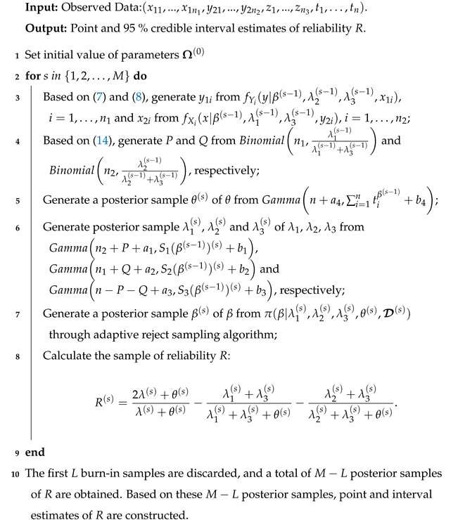
Gibbs sampling as a special MCMC method is an iteration algorithm, which is performed based on full conditional posteriors of the model parameters. In our case, each iteration in the Gibbs sampling algorithm includes two parts. In the first part, the unobserved data $(y_{11},\dots ,y_{1n_1},x_{21},\dots ,x_{2n_2})$ and binomial variables $(P,Q)$ are generated from (7), (8) and (14), respectively. Then, the posterior sample of the model parameters $\Omega$ are simulated from full conditional posteriors (12), (13) and (15), respectively. The detailed procedure of the Gibbs sampling algorithm can be summarized as follows (Algorithm 1).

Algorithm 1: Gibbs sampling.

5. Numerical Studies

5.1. A simulated Dataset

In order to assess the effectiveness of the proposed method, a dataset is simulated in this subsection, and we will show the detailed implementation process of Gibbs sampling as well as posterior diagnosis. Suppose that a system consists of two strength components in parallel and that the system is experienced by a stress variable, where the stress variable is denoted as T and the two strength components are denoted as $(X,Y)$. In addition, assume $T\sim Weibull(1.3,4)$, $(X,Y)\sim MOBW(1.3,0.9,1,1.3)$. That is, $\beta =1.3,{\eta }_1=0.9,{\eta }_2=1,{\eta }_3=1.3,\theta =4$. According to (5), the reliability of the system R is equal to 0.725. A group of data with sample size 50 is randomly generated from $Weibull(1.3,4)$ and $MOBW(1.3,0.9,1,1.3)$, respectively. The data generated from $MOBW(1.3,0.9,1,1.3)$ are $max(X,Y)$, and they are divided into three parts: $X>Y$, $X<Y$, and $X=Y$. The simulated data are listed in

Table 1. Observed data of stress variable T.

0.352	0.175	1.168	0.029	0.189	0.498	0.432	0.163	0.026	0.862
0.888	0.290	0.137	0.043	0.070	0.205	0.302	0.116	0.656	0.305
0.166	0.543	0.104	0.466	0.229	0.176	0.355	0.200	0.250	0.547
0.138	0.183	0.827	0.037	0.255	0.256	0.334	0.159	0.373	0.082
0.145	0.230	0.599	0.404	0.372	0.188	0.188	0.012	0.375	0.176

and

Table 2. Observed data of system strength.

$X>Y$	0.459	0.633	0.761	0.771	0.531	0.337	0.879	0.395	1.084	0.235
	0.435	1.402	1.443	1.368	0.411
$X<Y$	1.207	1.170	1.559	1.344	0.813	0.189	0.600	1.135	0.454	0.720
	1.128	0.509	0.821	0.630	0.699	0.443	0.346
$X=Y$	0.019	0.205	0.360	0.215	0.853	1.144	0.152	0.217	0.324	0.031
	0.537	0.263	0.238	0.706	0.356	0.380	0.365	0.535

.

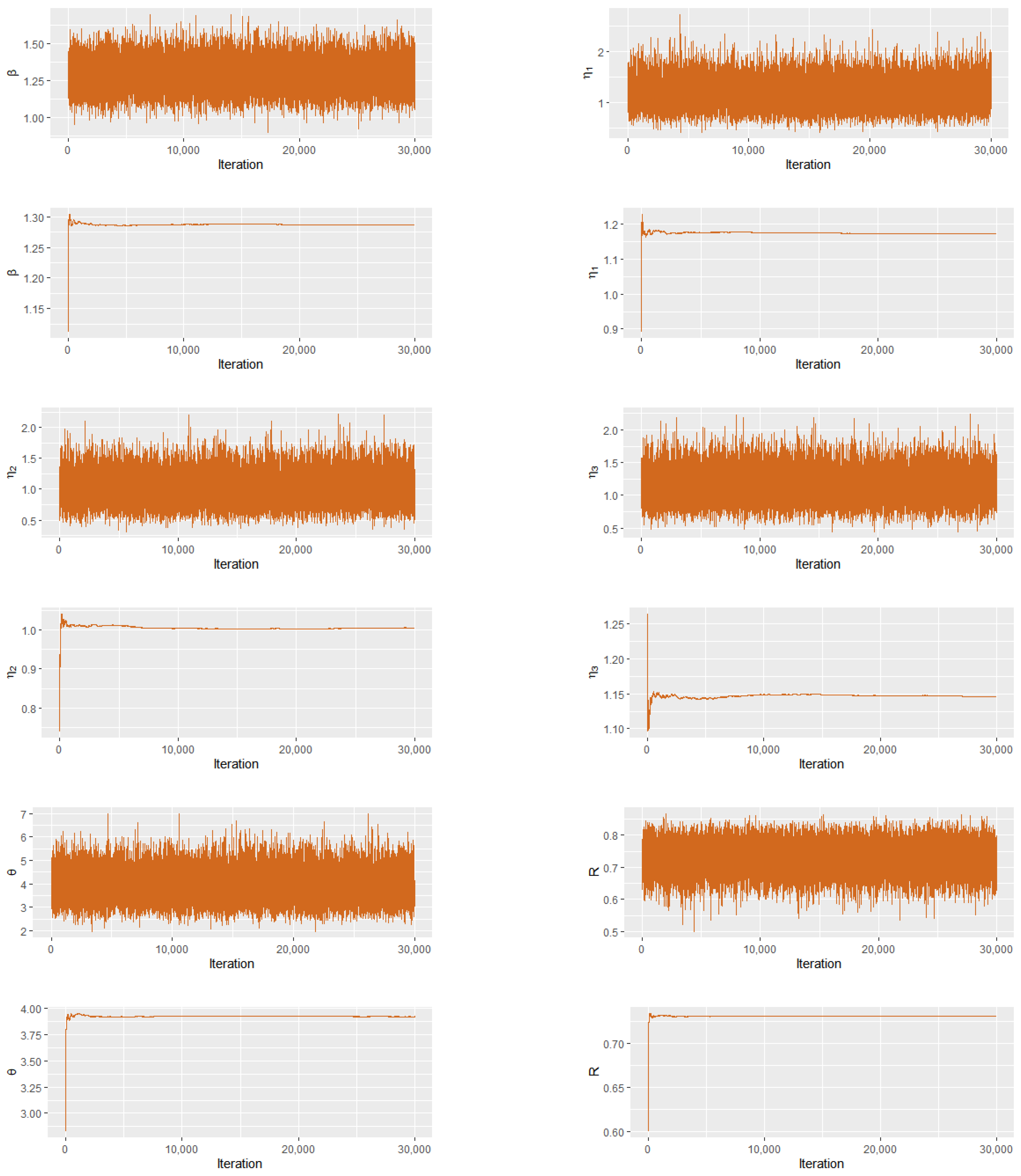
For performing Bayesian analysis, the priors of the model parameters $\Omega$ are assumed to be gamma distributions (10). We set the hyperparameters $a,b,a_j,b_j$, $j=1,\dots ,4$ in the priors as 0.001, which means that the priors have little information of the model parameters. Thus, Bayesian estimates are mainly determined by the data information. Then, the Gibbs sampling combined with data augmentation method (see Algorithm 1) is used to simplify the likelihood function of the model and to generate posterior samples of the parameters. A total of 30,000 posterior samples were generated by Gibbs sampling. The convergence of Gibbs sampling is checked by trace plots and ergodic mean plots, as are shown in Figure 1. By ergodic mean plots, we can intuitively judge the chains converge, because the ergodic means become stable after 1500 iterations. Additionally, Gelman and Rubin’s convergence diagnostic method is also utilized to check the Markov chain. Gelman and Rubin [32] proposed an index called potential scale reduction factor (PSRF) to measure whether there is a significant difference between intra-chain variances and inter-chain variances, so as to monitor the convergence of MCMC output. If the value of PSRF is close to 1, then the generated Markov chains are likely to have converged to one target distribution. For this aid, we generate posterior samples with three different initial values, and compute the value of PSRF, which is 1. This means that Markov chains have converged and the generated posterior samples with discarding the first 10,000 burn-in samples are from the true posterior distribution. Thus, the Bayesian estimates and the 95% credible interval of the model parameters and system reliability R can be obtained by the posterior samples, which are shown in

Table 3. Bayesian estimates of the model parameters and system reliability R based on simulated dataset.

Parameter	True	Estimate	95% Credible Interval
$\beta$	1.3	1.287	(1.097, 1.490)
${\eta }_1$	0.9	1.173	(0.711, 1.728)
${\eta }_2$	1	1.007	(0.594, 1.510)
${\eta }_3$	1.3	1.144	(0.736, 1.619)
$\theta$	4	3.919	(2.804, 5.238)
R	0.725	0.730	( 0.641, 0.811)

. As can be seen in Table 3, the estimated results are very close to the true values, which shows that the proposed method performs well.

5.2. Numerical Simulations with Different Scenarios

In this section, we will evaluate the proposed method through numerical simulation studies under different scenarios. Assume that the stress random variable $T\sim Weibull(\beta ,\theta )$, and the parallel system is composed of two components. Let X and Y represent the lifetime of the two components, respectively, and assume that $(X,Y)\sim MOBW(\beta ,{\lambda }_1,{\lambda }_2,{\lambda }_3)$. In the simulation studies, the shape parameter $\beta$ is set to 0.8, 1, 1.5, and 2.5, which can reflect the system with decreasing failure rate, constant failure rate, and increasing failure rate, respectively. The scale parameters $(\theta ,{\lambda }_1,{\lambda }_2,{\lambda }_3)$ are assumed to be (1, 3, 4, 3), (1, 1.5, 2, 4), and (0.9, 1.2, 0.8, 5). With the three settings of scale parameters, the corresponding true values of R are 0.40, 0.63, and 0.82, respectively. Thus, these settings can represent different levels of system reliability and can evaluate the effectiveness of the proposed method for the parallel systems with low, medium and high reliability. Finally, the sample size n is set to 20, 40, 60, 80, and 100. For each combination of parameter and sample size settings, 3000 samples are generated, and point and $95\%$ interval estimates of R based on Gibbs sampling algorithm are calculated for each sample.

The priors for the model parameters $\Omega$ are gamma distributions, and the hyperparameters $a,b,a_j,b_j$, $j=1,\dots ,4$ in the priors are also 0.001, as shown in the previous subsection. In the Gibbs sampling, the initial value of the model parameters ${\Omega }^{\left(0\right)}=({\beta }^{\left(0\right)},{\theta }^{\left(0\right)},{\lambda }_1^{\left(0\right)},{\lambda }_2^{\left(0\right)},{\lambda }_3^{\left(0\right)})$ is set to $(1,1,1,1,1)$, and the number of iteration M is 3000 with discarding the first 1500 burn-in samples. Then, for each generated sample, we can obtain the posterior mean and 95% credible interval of R are obtained based on the posterior sample of R. Based on the 3000 Bayesian point and interval estimates of R, we compute the the relative error (RE), mean squared error (MSE), as well as the length and frequency coverage probability (CP) of interval estimation. The results are listed in

Table 4. The results of Bayesian point and interval estimates of reliability R when $({\lambda }_1,{\lambda }_2,{\lambda }_3,{\lambda }_4)=(1,3,4,3)$.

$\mathit{\beta }$	n	RE	MSE	Length	CP
	20	0.0670	0.0041	0.2903	0.9790
	40	0.0451	0.0025	0.2099	0.9655
0.8	60	0.0339	0.0017	0.1726	0.9615
	80	0.0247	0.0013	0.1500	0.9625
	100	0.0212	0.0011	0.1343	0.9570
	20	0.0631	0.0041	0.2899	0.9765
	40	0.0404	0.0024	0.2096	0.9670
1	60	0.0280	0.0017	0.1724	0.9715
	80	0.0254	0.0014	0.1500	0.9570
	100	0.0217	0.0010	0.1344	0.9650
	20	0.0657	0.0042	0.2898	0.9765
	40	0.0414	0.0025	0.2096	0.9675
1.5	60	0.0281	0.0017	0.1722	0.9645
	80	0.0260	0.0014	0.1498	0.9605
	100	0.0218	0.0011	0.1343	0.9655
	20	0.0627	0.0044	0.2893	0.9745
	40	0.0407	0.0024	0.2096	0.9725
2.5	60	0.0268	0.0017	0.1720	0.9610
	80	0.0243	0.0013	0.1498	0.9630
	100	0.0175	0.0011	0.1341	0.9565

,

Table 5. The results of Bayesian point and interval estimates of reliability R when $({\lambda }_1,{\lambda }_2,{\lambda }_3,{\lambda }_4)=(1,1.5,2,4)$.

$\mathit{\beta }$	n	RE	MSE	Length	CP
	20	0.0471	0.0046	0.2899	0.9655
	40	0.0286	0.0027	0.2094	0.9560
0.8	60	0.0201	0.0018	0.1721	0.9585
	80	0.0152	0.0014	0.1494	0.9565
	100	0.0155	0.0011	0.1343	0.9595
	20	0.0436	0.0047	0.2897	0.9735
	40	0.0256	0.0024	0.2090	0.9700
1	60	0.0197	0.0017	0.1722	0.9655
	80	0.0172	0.0014	0.1497	0.9570
	100	0.0157	0.0011	0.1342	0.9510
	20	0.0426	0.0045	0.2895	0.972
	40	0.0282	0.0026	0.2093	0.9640
1.5	60	0.0225	0.0018	0.1723	0.9490
	80	0.0169	0.0014	0.1497	0.9500
	100	0.0141	0.0012	0.1340	0.9520
	20	0.0481	0.0047	0.2907	0.976
	40	0.0286	0.0027	0.2097	0.9640
2.5	60	0.0240	0.0018	0.1727	0.9585
	80	0.0151	0.0013	0.1498	0.9600
	100	0.0149	0.0011	0.1344	0.9550

and

Table 6. The results of Bayesian point and interval estimates of reliability R when $({\lambda }_1,{\lambda }_2,{\lambda }_3,{\lambda }_4)=(0.9,1.2,0.8,5)$.

$\mathit{\beta }$	n	RE	MSE	Length	CP
	20	0.0628	0.0052	0.2394	0.9105
	40	0.0373	0.0024	0.1661	0.9160
0.8	60	0.0277	0.0016	0.1345	0.9125
	80	0.0221	0.0011	0.1155	0.9205
	100	0.0192	0.0009	0.1031	0.9305
	20	0.0646	0.0054	0.2400	0.9135
	40	0.0375	0.0024	0.1663	0.9130
1	60	0.0285	0.0016	0.1344	0.9225
	80	0.0229	0.0011	0.1158	0.9205
	100	0.0207	0.0009	0.1035	0.9220
	20	0.0647	0.0053	0.2403	0.9185
	40	0.0372	0.0023	0.1659	0.9280
1.5	60	0.0296	0.0016	0.1349	0.9255
	80	0.0229	0.0011	0.1159	0.9295
	100	0.0192	0.0009	0.1030	0.9285
	20	0.0652	0.0053	0.2405	0.918
	40	0.0381	0.0023	0.1664	0.9245
2.5	60	0.0275	0.0015	0.1344	0.9185
	80	0.0237	0.0012	0.1160	0.9175
	100	0.0210	0.0009	0.1036	0.9140

. From the three tables, some points are quite clear and can be summarized as follows.

• As the sample size increases, the Re, MSE, and the length of interval estimate become smaller, and the frequentist CP is much closer to the nominal level 0.95.
• According to RE and MSE, the proposed method can provide accurate point estimation with small bias and variance.
• In terms of interval estimation, the Bayesian credible interval based on Gibbs sampling can yield good coverage, and even in the case of small sample size, the Bayesian credible interval can provide reasonable CP.

6. Conclusions

Based on the Marshall–Olkin bivariate Weibull distribution, this paper studies the reliability estimation of the multicomponent stress-strength model involving one stress and two correlated strength components from a parallel system. By introducing new latent variables in the model, the likelihood function is simplified to make the statistical inference available. Then, the Gibbs sampling algorithm is proposed to obtain Bayesian estimates of the model parameters as well as reliability of the system. Finally, the analysis of simulated dataset shows that the Bayesian estimates obtained by the proposed method are very close to the true value of reliability R, which shows that the effectiveness of the proposed method is very significant. In addition, the data simulation results show that even in the case of small samples, the point estimation and interval estimation of the proposed method are very effective, and with the increase of sample size, the interval coverage is very close to the nominal level 95%. It can be seen that the proposed method performs well under different settings. Thus, it can be applied to perform reliability analysis with multiple cases in practical applications. For example, with the development of science and technology, a variety of electronic devices have become an indispensable part of our life. Our model can be used to analyze the influence of charging voltage or temperature on battery reliability. In addition, it can also be used to analyze the influence of stress on the reliability of mechanical equipment, such as gears, turbo machines, aero-engines, etc.

References

1. Birnbaum, Z.W. On a use of Mann-Whitney statistics. In Contribution to the Theory of Statistics; University of California Press: Berkeley, CA, USA, 1956; Volume 1, pp. 13–17. [Google Scholar]
2. Birnbaum, Z.W.; McCarty, B.C. A distribution-free upper confidence bound for Pr{Y < X}, based on independent samples of X and Y. Ann. Math. Stat. 1958, 29, 558–562. [Google Scholar]
3. Kotz, S.; Lumelskii, Y.; Pensky, M. The Stress-Strength Model and Its Generalizations: Theory and Applications; World Scientific: Singapore, 2003. [Google Scholar]
4. Wang, B.X.; Geng, Y.; Zhou, J.X. Inference for the generalized exponential stress-strength model. Appl. Math. Model. 2018, 53, 267–275. [Google Scholar] [CrossRef]
5. Ghitany, M.E.; Al-Mutairi, D.K.; Aboukhamseen, S.M. Estimation of the reliability of a stress-strength system from power Lindley distributions. Commun. Stat.-Simul. Comput. 2015, 44, 118–136. [Google Scholar] [CrossRef]
6. Jose, J.K. Estimation of stress-strength reliability using discrete phase type distribution. Commun. Stat.-Theory Methods 2022, 51, 368–386. [Google Scholar] [CrossRef]
7. Panahi, H.; Asadi, S. Inference of stress-strength model for a Lomax distribution. Int. J. Math. Comput. Sci. 2011, 5, 937–940. [Google Scholar]
8. Sun, D.; Ghosh, M.; Basu, A.P. Bayesian analysis for a stress-strength system under noninformative priors. Can. J. Stat. 1998, 26, 323–332. [Google Scholar] [CrossRef]
9. Abbas, K.; Tang, Y.C. Objective Bayesian analysis of the Frechet stress–strength model. Stat. Probab. Lett. 2014, 84, 169–175. [Google Scholar] [CrossRef]
10. Sharma, V.K.; Singh, S.K.; Singh, U.; Agiwal, V. The inverse Lindley distribution: A stress-strength reliability model with application to head and neck cancer data. J. Ind. Prod. Eng. 2015, 32, 162–173. [Google Scholar] [CrossRef]
11. Chen, J.; Cheng, C. Reliability of stress–strength model for exponentiated Pareto distributions. J. Stat. Comput. Simul. 2017, 87, 791–805. [Google Scholar] [CrossRef]
12. Al-Mutairi, D.K.; Ghitany, M.E.; Kundu, D. Inferences on stress-strength reliability from Lindley distributions. Commun. Stat.-Theory Methods 2013, 42, 1443–1463. [Google Scholar] [CrossRef]
13. Singh, S.K.; Singh, U.; Sharma, V.K. Estimation on system reliability in generalized Lindley stress-strength model. J. Stat. Appl. Probab. 2014, 3, 61–75. [Google Scholar] [CrossRef]
14. Bhattacharyya, G.K.; Johnson, R.A. Estimation of reliability in multicomponent stress-strength model. J. Am. Stat. Assoc. 1974, 69, 966–970. [Google Scholar] [CrossRef]
15. Dey, S.; Mazucheli, J.; Anis, M.Z. Estimation of reliability of multicomponent stress–strength for a Kumaraswamy distribution. Commun. Stat.-Theory Methods 2017, 46, 1560–1572. [Google Scholar] [CrossRef]
16. Liu, Y.; Shi, Y.; Bai, X.; Zhan, P. Reliability estimation of a NM-cold-standby redundancy system in a multicomponent stress–strength model with generalized half-logistic distribution. Phys. A Stat. Mech. Its Appl. 2018, 490, 231–249. [Google Scholar] [CrossRef]
17. Jha, M.K.; Dey, S.; Alotaibi, R.M.; Tripathi, Y.M. Reliability estimation of a multicomponent stress-strength model for unit Gompertz distribution under progressive Type II censoring. Qual. Reliab. Eng. Int. 2020, 36, 965–987. [Google Scholar] [CrossRef]
18. Rasekhi, M.; Saber, M.M.; Yousof, H.M. Bayesian and classical inference of reliability in multicomponent stress-strength under the generalized logistic model. Commun. Stat.-Theory Methods 2020, 50, 5114–5125. [Google Scholar] [CrossRef]
19. Wang, L.; Dey, S.; Tripathi, Y.M.; Wu, S.J. Reliability inference for a multicomponent stress–strength model based on Kumaraswamy distribution. J. Comput. Appl. Math. 2020, 376, 377–427. [Google Scholar] [CrossRef]
20. Kang, S.G.; Lee, W.D.; Kim, Y. Objective Bayesian analysis for generalized exponential stress–strength model. Comput. Stat. 2021, 36, 2079–2109. [Google Scholar] [CrossRef]
21. Luo, C.; Shen, L.; Xu, A. Modelling and estimation of system reliability under dynamic operating environments and lifetime ordering constraints. Reliab. Eng. Syst. Saf. 2022, 218, 108136. [Google Scholar] [CrossRef]
22. Kızılaslan, F.; Nadar, M. Estimation of reliability in a multicomponent stress–strength model based on a bivariate Kumaraswamy distribution. Stat. Pap. 2018, 59, 307–340. [Google Scholar] [CrossRef]
23. Kundu, D.; Gupta, A.K. Bayes estimation for the Marshall-Olkin bivariate Weibull distribution. Comput. Stat. Data Anal. 2013, 57, 271–281. [Google Scholar] [CrossRef]
24. Bai, X.; Shi, Y.; Liu, Y.; Liu, B. Reliability estimation of multicomponent stress–strength model based on copula function under progressively hybrid censoring. J. Comput. Appl. Math. 2018, 344, 100–114. [Google Scholar] [CrossRef]
25. Nadar, M.; Kızılaslan, F. Estimation of reliability in a multicomponent stress-strength model based on a Marshall-Olkin bivariate Weibull distribution. IEEE Trans. Reliab. 2015, 65, 370–380. [Google Scholar] [CrossRef]
26. Mokhlis, N.A.; Khames, S.K. Reliability of multi-component stress–strength models. J. Egypt. Math. Soc. 2011, 19, 106–111. [Google Scholar] [CrossRef] [Green Version]
27. Zhu, T. Reliability estimation of s-out-of-k system in a multicomponent stress–strength dependent model based on copula function. J. Comput. Appl. Math. 2022, 404, 113920. [Google Scholar] [CrossRef]
28. Ghosh, J.K.; Delampady, M.; Samanta, T. An Introduction to Bayesian Analysis: Theory and Methods; Springer: New York, NY, USA, 2006. [Google Scholar]
29. Kundu, D.; Nekoukhou, V. On bivariate discrete Weibull distribution. Commun. Stat.-Theory Methods 2019, 48, 3464–3481. [Google Scholar] [CrossRef] [Green Version]
30. Marshall, A.W.; Olkin, I. A multivariate exponential distribution. J. Am. Stat. Assoc. 1967, 62, 30–44. [Google Scholar] [CrossRef]
31. Kundu, D.; Dey, A.K. Estimating the parameters of the Marshall-Olkin bivariate Weibull distribution by EM algorithm. Comput. Stat. Data Anal. 2009, 53, 956–965. [Google Scholar] [CrossRef] [Green Version]
32. Gelman, A.; Rubin, D.B. Inference from iterative simulation using multiple sequences. Stat. Sci. 1992, 7, 457–511. [Google Scholar] [CrossRef]
Figure 1. Trace and ergodic mean plots of posterior samples.
Systems 10 00196 g001