Evolutionary Game Analysis between Local Government and Enterprises on Bridge Employment from the Perspective of Dynamic Incentive and Punishment
Abstract
:1. Introduction
2. Literature Review
3. Materials and Methods
3.1. Theoretical Basis
3.2. Problem Description
3.3. Model Establishment
4. Results
4.1. Static Equilibrium Analysis
4.1.1. Static Equilibrium Analysis of Local Government
- (1)
- If , we can have , and , then is the stable point.
- (2)
- If , we can have , and , then is the stable point.
4.1.2. Static Equilibrium Analysis of Enterprises
- (1)
- If , we can have , then is the stable point.
- (2)
- If , we can have , then is the stable point.
- (3)
- If , there are two scenarios to discuss:
- (i)
- if , then , , is the stable point.
- (ii)
- if , then , , is the stable point.
4.1.3. Static Equilibrium Analysis of the System
- (1)
- The system always has four fixed equilibrium points, namely , , , and .
- (2)
- If and , the system has another equilibrium point , where , .
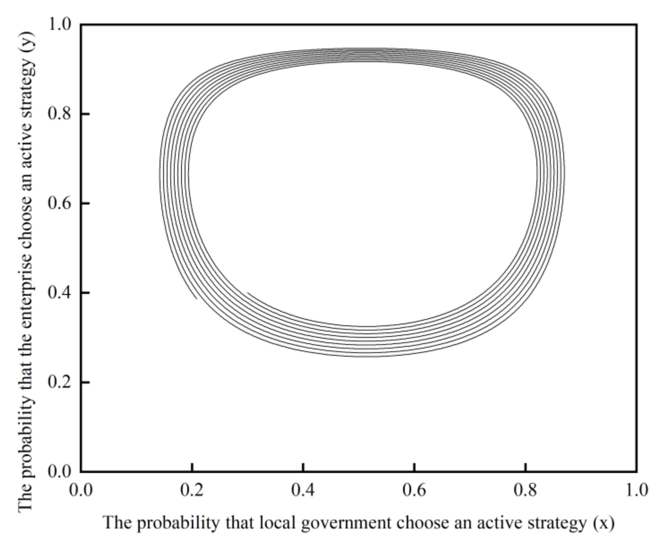
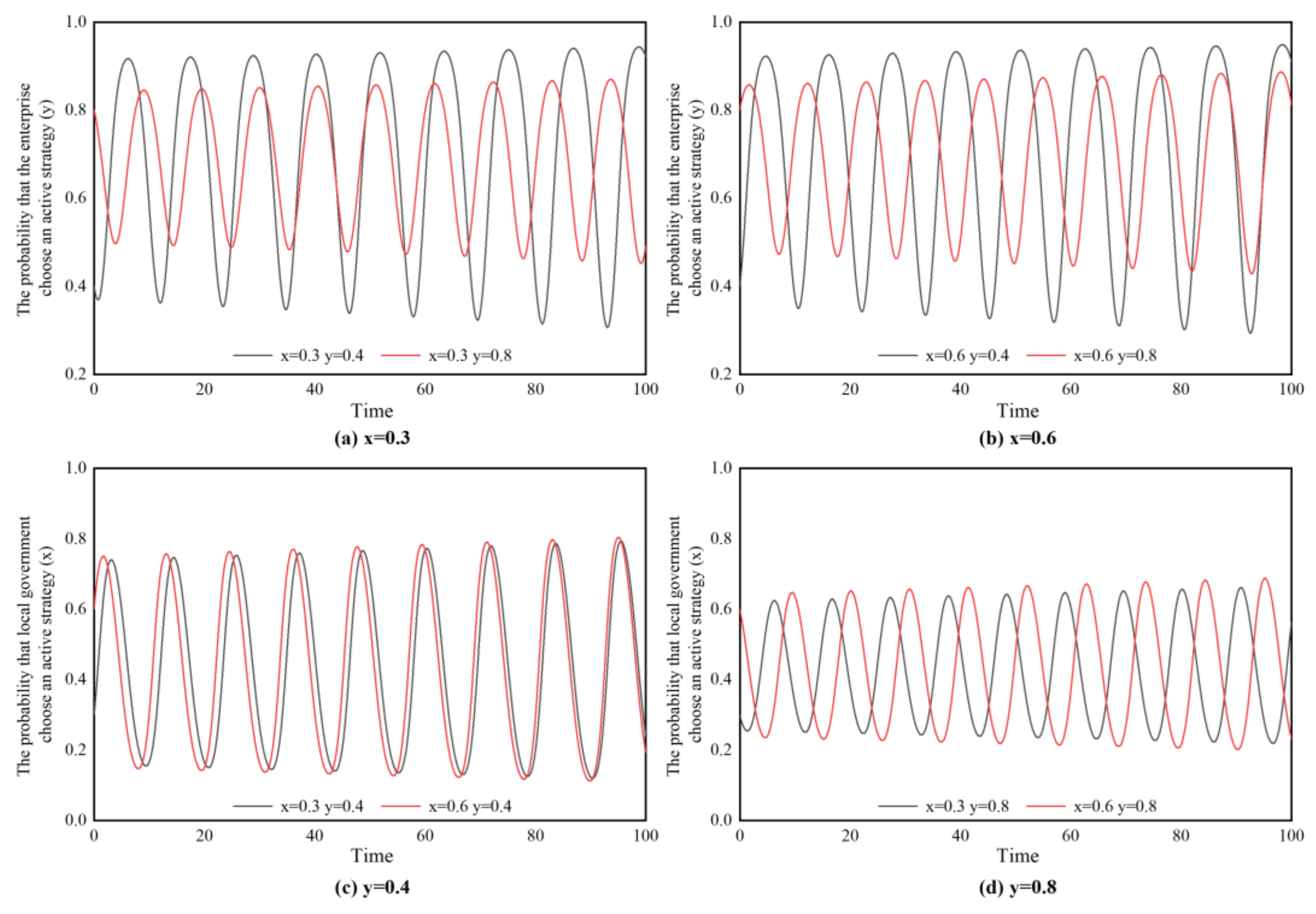
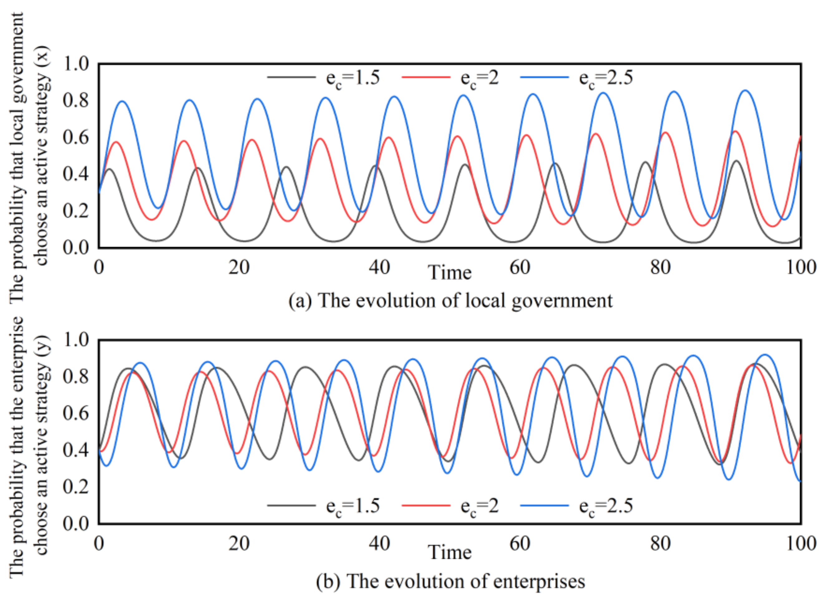
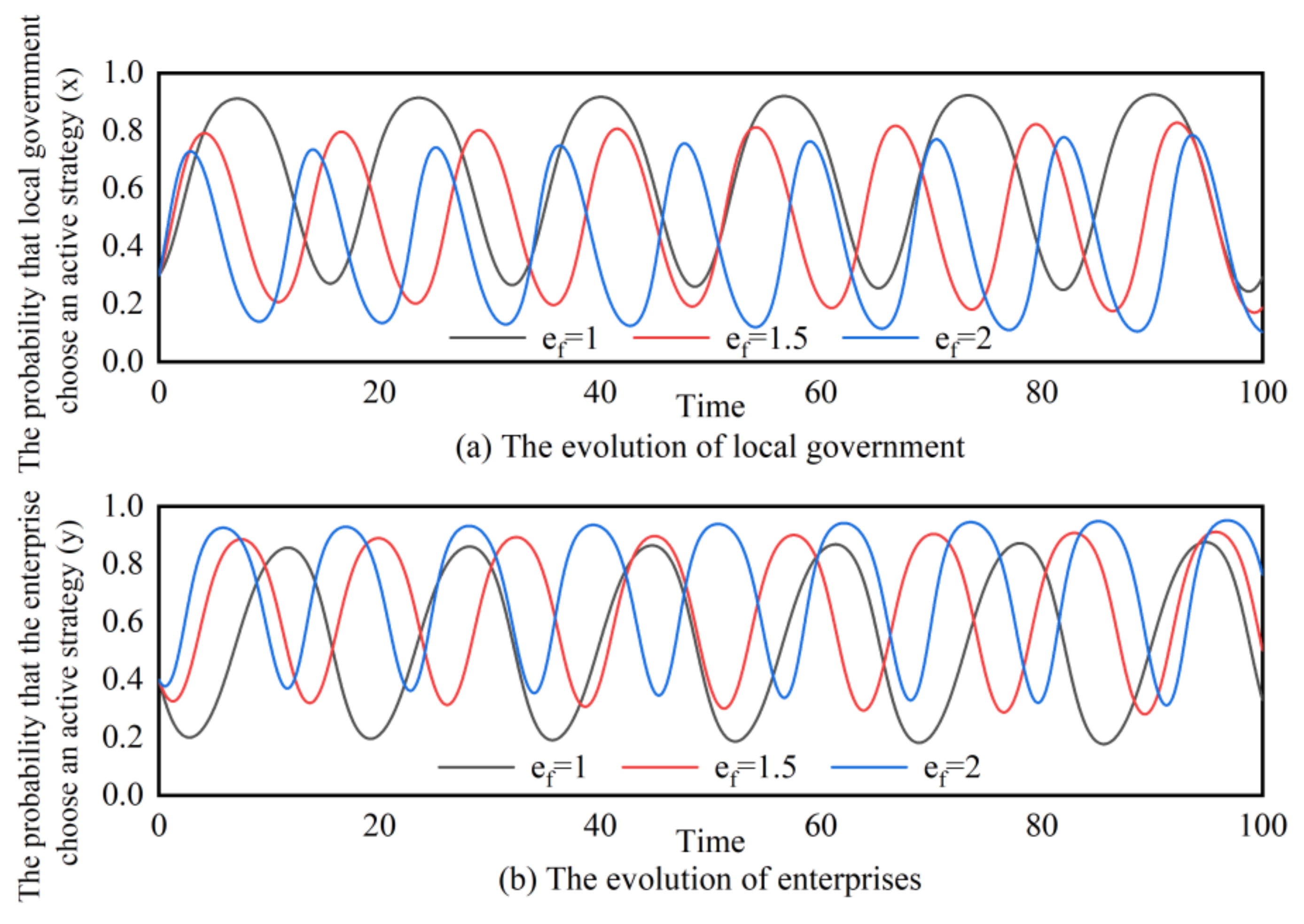
4.1.4. Simulation Analysis
4.2. Dynamic Equilibrium Analysis
4.2.1. Dynamic Incentive Mechanism
- (1)
- The dynamic incentive system always has three fixed equilibrium points, namely , , and .
- (2)
- For , are equilibrium points of the dynamic incentive system.
- (2)
- If and , the dynamic incentive system has another equilibrium point , where , .
- (i)
- , , and .
- (ii)
- and .
4.2.2. Dynamic Punishment Mechanism
- (1)
- The system always has four fixed equilibrium points, namely , , , and .
- (2)
- If and , the system has another equilibrium point , where , .
- (i)
- , , , and .
- (ii)
- and .
4.2.3. Dynamic Incentive and Punishment Mechanism
- (1)
- The system always has four fixed equilibrium points, namely , , , and .
- (2)
- If and , the system has another equilibrium point , where , .
- (i)
- , , and .
- (ii)
- and .
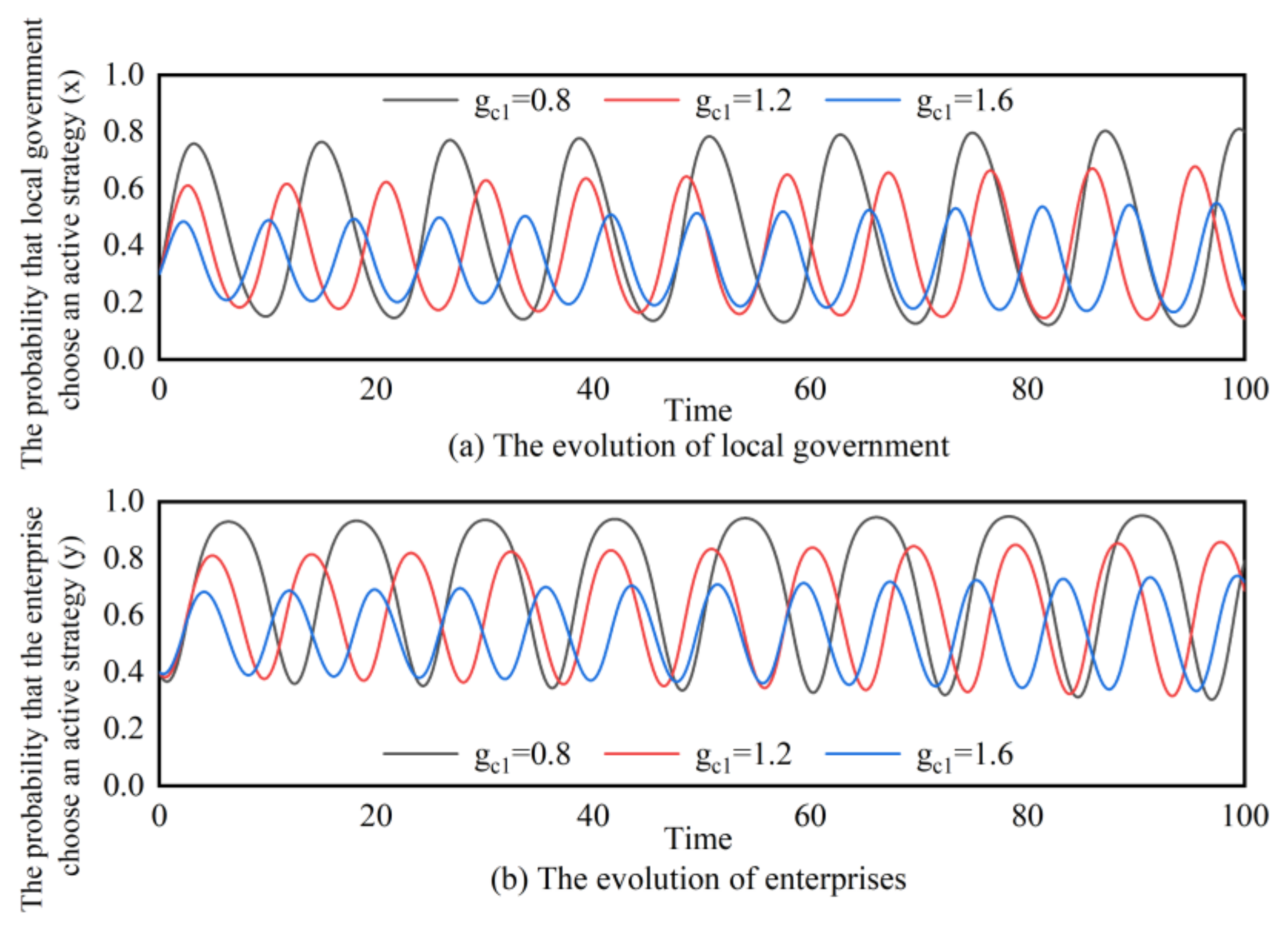
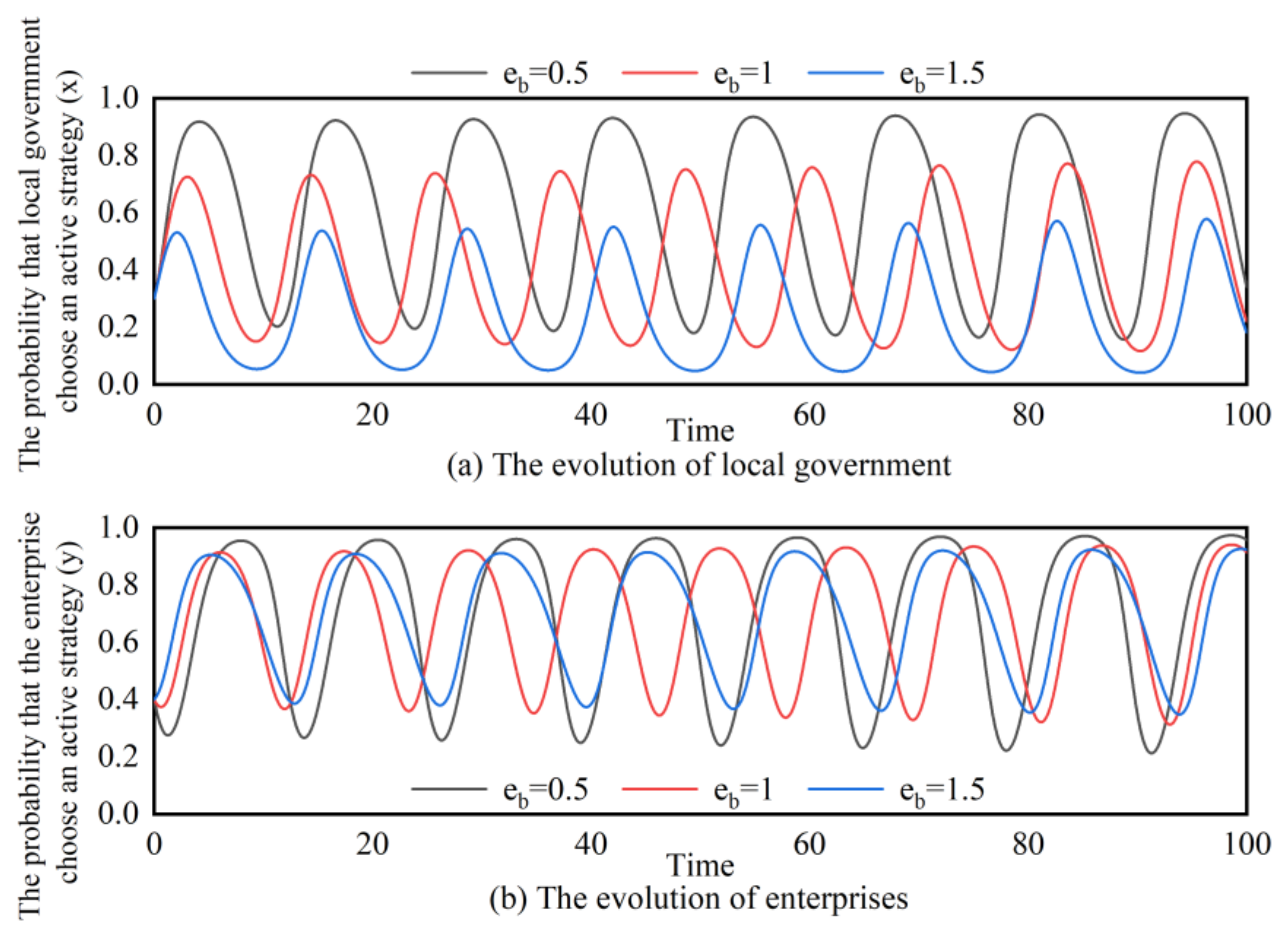
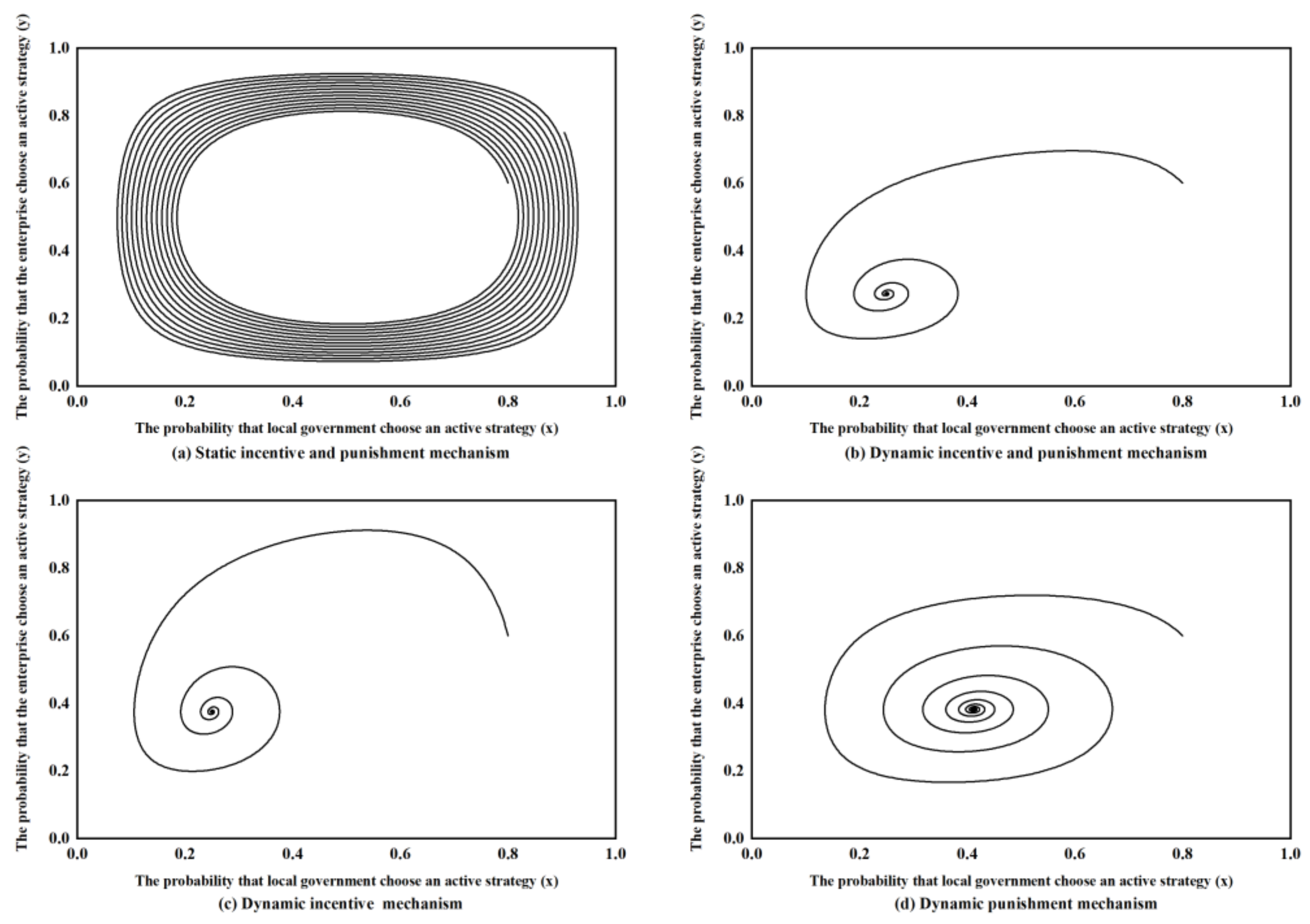
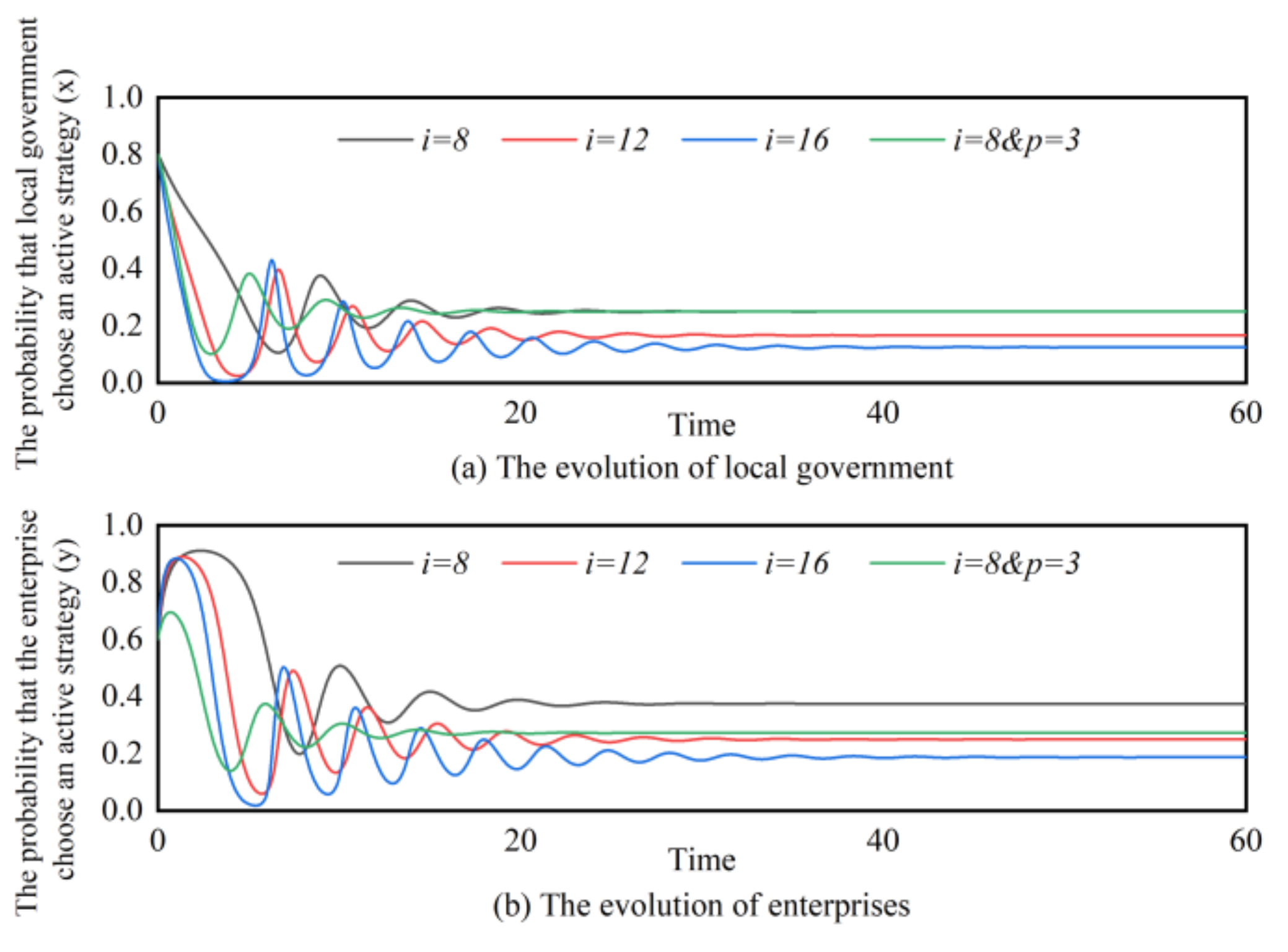
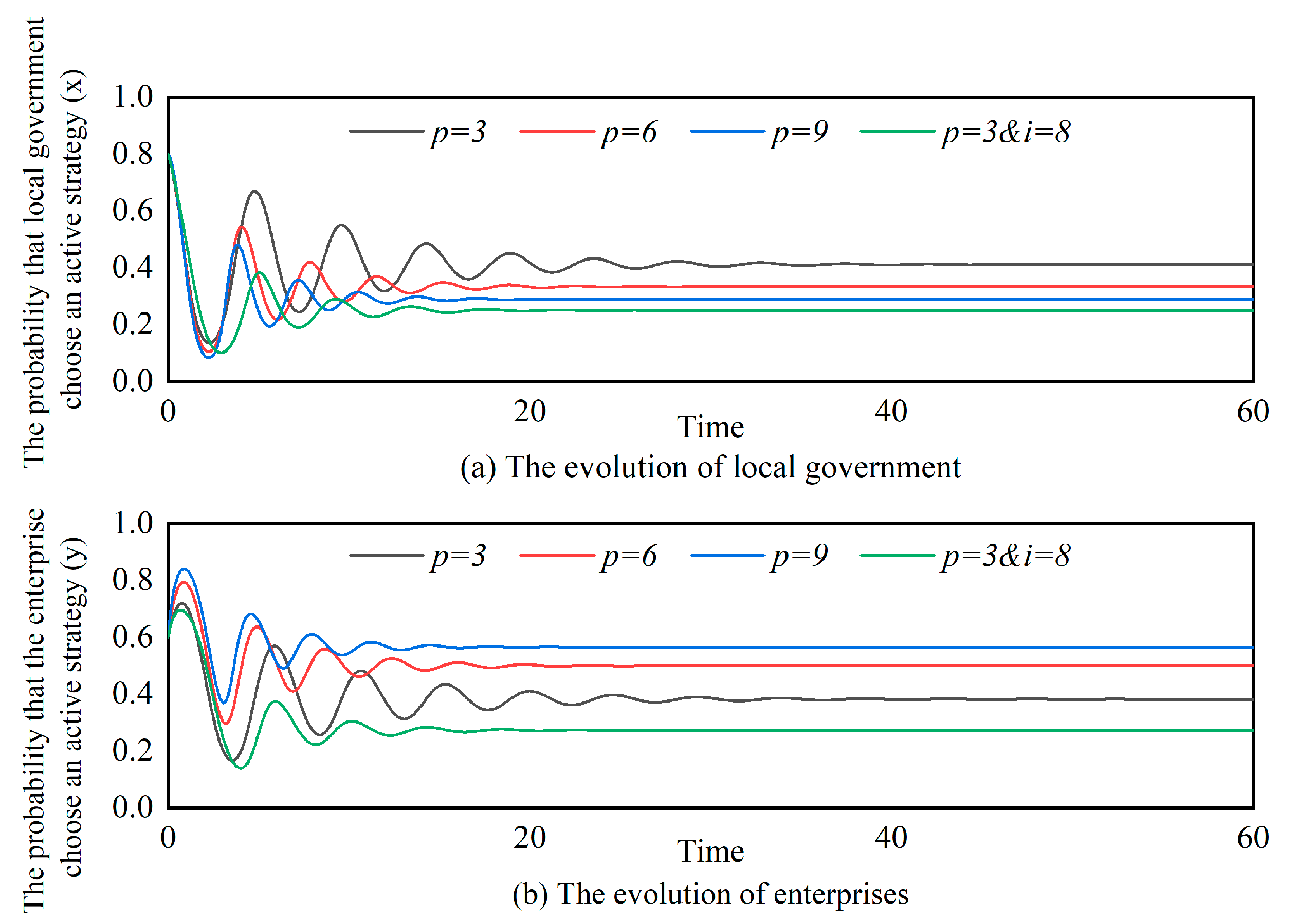
4.2.4. Simulation Analysis
5. Discussion
5.1. Management Implications
5.2. Strengths, Limitations, and Future Research
6. Conclusions
Author Contributions
Funding
Data Availability Statement
Conflicts of Interest
References
- WHO. Active Ageing: A Policy Framework; World Health Organization: Geneva, Switzerland; Madrid, Spain, 2002. [Google Scholar]
- Boulton-Lewis, G.M.; Buys, L.; Lovie-Kitchin, J. Learning and Active Aging. Educ. Gerontol. 2006, 32, 271–282. [Google Scholar] [CrossRef]
- Doeringer, P.B. Bridges to Retirement: Older Workers in a Changing Labor Market; Cornell University Press: Ithaca, Greece, 1990. [Google Scholar]
- Gobeski, K.T.; Beehr, T.A. How retirees work: Predictors of different types of bridge employment. J. Organ. Behav. 2009, 30, 401–425. [Google Scholar] [CrossRef]
- Yaohui, Z.; John, S.; Gonghuan, Y. China Health and Retirement Longitudinal Study; Institute of Social Science Survey, Peking University: Peking, China, 2015. [Google Scholar] [CrossRef]
- Platts, L.G.; Corna, L.M.; Worts, D.; McDonough, P.; Price, D.; Glaser, K. Returns to work after retirement: A prospective study of unretirement in the United Kingdom. Ageing Soc. 2017, 39, 439–464. [Google Scholar] [CrossRef]
- Settels, J.; McMullin, J. Gender and Relationship Status Interaction and Likelihood of Return to Work Post-Retirement. Can. J. Aging 2017, 36, 366–385. [Google Scholar] [CrossRef]
- Maestas, N. Back to work expectations and realizations of work after retirement. J. Hum. Resour. 2010, 45, 718–748. [Google Scholar] [CrossRef]
- Quinn, J. Work, retirement, and the encore career: Elders and the future of the American workforce. Generations 2010, 34, 45–55. [Google Scholar]
- Beehr, T.A.; Bennett, M.M. Working After Retirement: Features of Bridge Employment and Research Directions. Work. Aging Retire. 2014, 1, 112–128. [Google Scholar] [CrossRef]
- You, M.; Li, S.; Li, D.; Cao, Q.; Xu, F. Evolutionary game analysis of coal-mine enterprise internal safety inspection system in China based on system dynamics. Resour. Policy 2020, 67, 101673. [Google Scholar] [CrossRef]
- Fan, R.; Wang, Y.; Lin, J. Study on Multi-Agent Evolutionary Game of Emergency Management of Public Health Emergencies Based on Dynamic Rewards and Punishments. Int. J. Environ. Res. Public Health 2021, 18, 8278. [Google Scholar] [CrossRef]
- Meng, Q.; Liu, Y.; Li, Z.; Wu, C. Dynamic reward and penalty strategies of green building construction incentive: An evolutionary game theory-based analysis. Environ. Sci. Pollut. Res. 2021, 28, 44902–44915. [Google Scholar] [CrossRef]
- Shultz, K.S. Bridge Employment: Work after Retirement; Springer: New York, NY, USA, 2003; pp. 214–241. [Google Scholar]
- Feldman, D.C. The Decision to Retire Early: A Review and Conceptualization. Acad. Manag. Rev. 1994, 19, 285–311. [Google Scholar] [CrossRef]
- Ulrich, L.B.; Brott, P.E. Older Workers and Bridge Employment: Redefining Retirement. J. Employ. Couns. 2005, 42, 159–170. [Google Scholar] [CrossRef]
- Wang, M. Profiling retirees in the retirement transition and adjustment process: Examining the longitudinal change patterns of retirees’ psychological well-being. J. Appl. Psychol. 2007, 92, 455–474. [Google Scholar] [CrossRef]
- Björklund Carlstedt, A.; Jacobsson, G.; Bjursell, C.; Nystedt, P.; Sternäng, O. Staffing agency: A bridge to working during retirement. Work 2022, 72, 529–537. [Google Scholar] [CrossRef]
- Kim, E. Korean baby boomer retirees’ bridge employment experiences in community service jobs. Educ. Gerontol. 2021, 47, 151–159. [Google Scholar] [CrossRef]
- Peng, Y. A two-study examination of age discrimination, work meaningfulness, and bridge employment intentions. Career Dev. Int. 2022, 27, 391–407. [Google Scholar] [CrossRef]
- Lorenz, S.; Zwick, T.; Bruns, M. Beware of the employer: Financial incentives for employees may fail to prolong old-age employment. J. Econ. Ageing 2022, 21, 100363. [Google Scholar] [CrossRef]
- Mazumdar, B.; Warren, A.; Dupré, K.; Brown, T. Employment expectations: Examining the effect of psychological contract fulfillment on bridge employees’ personal and work attitudes. Pers. Rev. 2022. ahead-of-print. [Google Scholar] [CrossRef]
- Raymo, J.M.; Liang, J.; Sugisawa, H.; Kobayashi, E.; Sugihara, Y. Work at Older Ages in Japan: Variation by Gender and Employment Status. J. Gerontol. Ser. B 2004, 59, S154–S163. [Google Scholar] [CrossRef]
- Jones, D.A.; McIntosh, B.R. Organizational and occupational commitment in relation to bridge employment and retirement intentions. J. Vocat. Behav. 2010, 77, 290–303. [Google Scholar] [CrossRef]
- Kerr, G.; Armstrong-Stassen, M. The Bridge to Retirement: Older Workers’ Engagement in Post-Career Entrepreneurship and Wage-and-Salary Employment. J. Entrep. 2011, 20, 55–76. [Google Scholar] [CrossRef]
- Wang, M.; Adams, G.A.; Beehr, T.A.; Shultz, K.S. Bridge Employment and Retirement; Information Age Publishing: Charlotte, NC, USA, 2009. [Google Scholar]
- Mariappanadar, S. Do retirement anxieties determine bridge employment preference? Pers. Rev. 2013, 42, 176–204. [Google Scholar] [CrossRef]
- Zhan, Y.; Wang, M.; Yao, X. Domain specific effects of commitment on bridge employment decisions: The moderating role of economic stress. Eur. J. Work. Organ. Psychol. 2013, 22, 362–375. [Google Scholar] [CrossRef]
- Garcia, P.R.J.M.; Amarnani, R.K.; Bordia, P.; Restubog, S.L.D. When support is unwanted: The role of psychological contract type and perceived organizational support in predicting bridge employment intentions. J. Vocat. Behav. 2021, 125, 103–120. [Google Scholar] [CrossRef]
- Wang, M.; Zhan, Y.; Liu, S.; Shultz, K.S. Antecedents of bridge employment: A longitudinal investigation. J. Appl. Psychol. 2008, 93, 818–930. [Google Scholar] [CrossRef]
- Yin, R.; Xin, Y.; Bhura, M.; Wang, Z.; Tang, K. Bridge Employment and Longevity: Evidence From a 10-Year Follow-Up Cohort Study in 0.16 Million Chinese. J. Gerontol. Ser. B 2022, 77, 750–758. [Google Scholar] [CrossRef]
- Zhan, Y.; Wang, M.; Liu, S.; Shultz, K.S. Bridge employment and retirees’ health: A longitudinal investigation. J. Occup. Health Psychol. 2009, 14, 374–389. [Google Scholar] [CrossRef]
- Kim, S.; Feldman, D.C. Working in retirement: The antecedents of bridge employment and its consequences for quality of life in retirement. Acad. Manag. J. 2000, 43, 1195–1210. [Google Scholar] [CrossRef]
- Cahill, K.E.; Giandrea, M.D.; Quinn, J.F. Bridge employment. In The Oxford Handbook of Retirement; Oxford University Press: Oxford, UK, 2013. [Google Scholar] [CrossRef]
- Mazumdar, B.; Warren, A.M.; Brown, T.C. Bridge employment: Understanding the expectations and experiences of bridge employees. Hum. Resour. Manag. J. 2021, 31, 575–591. [Google Scholar] [CrossRef]
- Zhan, Y.; Wang, M.; Shi, J. Retirees’ motivational orientations and bridge employment: Testing the moderating role of gender. J. Appl. Psychol. 2015, 100, 1319–1331. [Google Scholar] [CrossRef]
- Lahlouh, K.; Lacaze, D.; Huaman-Ramirez, R. Bridge employment and full retirement intentions: The role of person-environment fit. Pers. Rev. 2019, 48, 1469–1490. [Google Scholar] [CrossRef]
- Peng, Y.; Xu, X.; Jex, S.M.; Chen, Y. The Roles of Job-Related Psychosocial Factors and Work Meaningfulness in Promoting Nurses’ Bridge Employment Intentions. J. Career Dev. 2020, 47, 701–716. [Google Scholar] [CrossRef]
- Loretto, W.; White, P. Employers’ attitudes, practices and policies towards older workers. Hum. Resour. Manag. J. 2006, 16, 313–330. [Google Scholar] [CrossRef]
- Conen, W.S.; Henkens, K.; Schippers, J. Employers’ attitudes and actions towards the extension of working lives in Europe. Int. J. Manpow. 2012, 33, 648–665. [Google Scholar] [CrossRef]
- Oude Mulders, J.; van Dalen, H.P.; Henkens, K.; Schippers, J. How Likely are Employers to Rehire Older Workers after Mandatory Retirement? A Vignette Study among Managers. Economist 2014, 162, 415–431. [Google Scholar] [CrossRef]
- Karpinska, K.; Henkens, K.; Schippers, J. The recruitment of early retirees: A vignette study of the factors that affect managers’ decisions. Ageing Soc. 2011, 31, 570–589. [Google Scholar] [CrossRef]
- Templer, A.; Armstrong-Stassen, M.; Cattaneo, J. Antecedents of older workers’ motives for continuing to work. Career Dev. Int. 2010, 15, 479–500. [Google Scholar] [CrossRef]
- Feldman, D.C.; Kim, S. Bridge Employment During Retirement: A Field Study of Individual and Organizational Experiences with Post-Retirement Employment. Hum. Resour. Plan. 2000, 23, 14–25. [Google Scholar]
- Mazumdar, B.; Warren, A.M.; Dupré, K.E. Extending the understanding of bridge employment: A critical analysis. Pers. Rev. 2018, 47, 1345–1361. [Google Scholar] [CrossRef]
- Alcover, C.-M.; Topa, G.; Parry, E. Bridge Employment: Lessons Learned and Future Prospects for Research and Practice; Routledge: Oxford, UK, 2014; pp. 295–316. [Google Scholar]
- Ashford, S.J.; George, E.; Blatt, R. Old assumptions, new work: The opportunities and challenges of research on nonstandard employment. Acad. Manag. Ann. 2007, 1, 65–117. [Google Scholar] [CrossRef]
- Smith, J.M.; Price, G.R. The logic of animal conflict. Nature 1973, 246, 15–18. [Google Scholar] [CrossRef]
- Taylor, P.D.; Jonker, L.B. Evolutionary stable strategies and game dynamics. Math. Biosci. 1978, 40, 145–156. [Google Scholar] [CrossRef]
- Smith, J.M. The theory of games and the evolution of animal conflicts. J. Theor. Biol. 1974, 47, 209–221. [Google Scholar] [CrossRef]
- Zhiwen, Z.; Yujun, X.; Junxing, L.; Limin, G.; Long, W. Supply Chain Logistics Information Collaboration Strategy Based on Evolutionary Game Theory. IEEE Access 2020, 8, 46102–46120. [Google Scholar] [CrossRef]
- Pan, X.Y.; Gelfand, M.; Nau, D. Integrating Evolutionary Game Theory and Cross-Cultural Psychology to Understand Cultural Dynamics. Am. Psychol. 2021, 76, 1054–1066. [Google Scholar] [CrossRef]
- Krapohl, S.; Ocelík, V.; Walentek, D.M. The instability of globalization: Applying evolutionary game theory to global trade cooperation. Public Choice 2021, 188, 31–51. [Google Scholar] [CrossRef]
- Dong, J.; Yan, S. Evolutionary game analysis between employees and employers about working overtime from the perspective of information asymmetry. BMC Psychol. 2022, 10, 95–108. [Google Scholar] [CrossRef]
- Friedman, D. On economic applications of evolutionary game theory. J. Evol. Econ. 1998, 8, 15–43. [Google Scholar] [CrossRef]

| Parameters | Descriptions | Notes |
|---|---|---|
| The probability that the government actively implements rewards and punishments. | ||
| Additional benefits for the government. | ||
| Direct cost to the government. | ||
| Indirect cost to the government. | ||
| Additional cost to the government. | ||
| The probability that enterprises actively respond to government policies. | ||
| Profits earned by the enterprise. | ||
| Indirect benefits to the enterprise. | ||
| The cost consumed by the enterprise. | ||
| Fines imposed on enterprises. |
| Local Government | Enterprises | |
|---|---|---|
| Active (y) | Pasive (1 − y) | |
| Active (x) | ||
| Passive (1 − x) | ||
| Equilibrium Points | DetJ | Sign | TrJ | Sign | Result |
|---|---|---|---|---|---|
| Uncertain | Saddle point | ||||
| Uncertain | Saddle point | ||||
| Uncertain | Saddle point | ||||
| Uncertain | Saddle point | ||||
| 0 | 0 | Central point |
| Local Government | Enterprises | |
|---|---|---|
| Active (y) | Passive (1 − y) | |
| Active (x) | ||
| Passive (1 − x) | ||
| Local Government | Enterprises | |
|---|---|---|
| Active (y) | Passive (1 − y) | |
| Active (x) | ||
| Passive (1 − x) | ||
| Local Government | Enterprises | |
|---|---|---|
| Active (y) | Passive (1 − y) | |
| Active (x) | ||
| Passive (1 − x) | ||
Publisher’s Note: MDPI stays neutral with regard to jurisdictional claims in published maps and institutional affiliations. |
© 2022 by the authors. Licensee MDPI, Basel, Switzerland. This article is an open access article distributed under the terms and conditions of the Creative Commons Attribution (CC BY) license (https://creativecommons.org/licenses/by/4.0/).
Share and Cite
Dong, J.; Yan, S.; Yang, X. Evolutionary Game Analysis between Local Government and Enterprises on Bridge Employment from the Perspective of Dynamic Incentive and Punishment. Systems 2022, 10, 115. https://doi.org/10.3390/systems10040115
Dong J, Yan S, Yang X. Evolutionary Game Analysis between Local Government and Enterprises on Bridge Employment from the Perspective of Dynamic Incentive and Punishment. Systems. 2022; 10(4):115. https://doi.org/10.3390/systems10040115
Chicago/Turabian StyleDong, Junjie, Shumin Yan, and Xiaowei Yang. 2022. "Evolutionary Game Analysis between Local Government and Enterprises on Bridge Employment from the Perspective of Dynamic Incentive and Punishment" Systems 10, no. 4: 115. https://doi.org/10.3390/systems10040115
APA StyleDong, J., Yan, S., & Yang, X. (2022). Evolutionary Game Analysis between Local Government and Enterprises on Bridge Employment from the Perspective of Dynamic Incentive and Punishment. Systems, 10(4), 115. https://doi.org/10.3390/systems10040115


