The Worst Performance Rule as Moderation: New Methods for Worst Performance Analysis

Abstract

Worst performance in cognitive processing tasks shows larger relationships to general intelligence than mean or best performance. This so called Worst Performance Rule (WPR) is of major theoretical interest for the field of intelligence research, especially for research on mental speed. In previous research, the increases in correlations between task performance and general intelligence from best to worst performance were mostly described and not tested statistically. We conceptualized the WPR as moderation, since the magnitude of the relation between general intelligence and performance in a cognitive processing task depends on the performance band or percentile of performance. On the one hand, this approach allows testing the WPR for statistical significance and on the other hand, it may simplify the investigation of possible constructs that may influence the WPR. The application of two possible implementations of this approach is shown and compared to results of a traditional worst performance analysis. The results mostly replicate the WPR. Beyond that, a comparison of results on the level of unstandardized relationships (e.g., covariances or unstandardized regression weights) to results on the level of standardized relationships (i.e., correlations) indicates that increases in the inter-individual standard deviation from best to worst performance may play a crucial role for the WPR. Altogether, conceptualizing the WPR as moderation provides a new and straightforward way to conduct Worst Performance Analysis and may help to incorporate the WPR more prominently into empirical practice of intelligence research.

1. Introduction

A wealth of research has reported results that support a consistent and moderate to mediocre relationship between mental speed and general intelligence (for a review, see [1]). Across a variety of different tasks measuring mental speed, Sheppard and Vernon [1] reported an average correlation of $r=-.24$ between response times and measures of general intelligence. This indicates that faster speed of information processing is associated with greater general intelligence. Beyond that, this relationship between mental speed and intelligence is not only present in behavioral measures of mental speed but in neural measures of mental speed, such as latencies of event-related potentials, as well [2]. However, most of these results rely on mean scores for mental speed.

Recent empirical results have suggested that inter-individual differences in mean performance on tasks measuring mental speed or memory capacity may not be best suited to predict general intelligence. In fact, it seems that within such tasks worst performance is more indicative for general intelligence [3]. In detail, performance in various processing speed or memory tasks was ranked from fastest to slowest reaction times (RTs) or best to worst memory recall. Then, means of different RT bands or best and worst memory performance were correlated with a measure of general intelligence. The absolute size of these correlations mostly increased from best to worst performance, suggesting that worst performance is more closely related to general intelligence than mean or best performance. This phenomenon is called the worst performance rule (WPR) [4]. Although a few studies replicated this phenomenon [5,6,7,8,9,10], it has yet to be acknowledged adequately in the field of intelligence research.

In previous research, the analysis of the WPR, or so called worst performance analysis (WPA), mostly described increases in correlations between performance in cognitive processing tasks and general intelligence from best to worst performance instead of providing an adequate statistical test for this phenomenon (for a detailed review, see [3]). The present work conceptualizes the WPR as moderation and introduces new approaches to analyze and test the WPR for statistical significance. These analyses try to overcome the rather descriptive approach of formerly published WPA and offer new possibilities to search for empirical foundations of the WPR. The here presented analysis may hence constitute a useful step towards an accurate test for the WPR that may in turn help to better distinguish between different theoretical explanations for the WPR in future empirical research.

1.1. The Phenomenon of the Worst Performance Rule

The WPR was first explicitly described by Larson and Alderton [4] who showed that correlations of general intelligence with RTs in a simple reaction time paradigm increased from best ($r_{\text{BP}}=-.20$) to worst performance ($r_{\text{WP}}=-.37$). This initiated a number of conceptually associated studies [5,6,7,8,9,10,11] with different related tasks of which all but one [11] reproduced the basic phenomenon of the WPR.

Interestingly, the WPR did not only occur in speeded processing tasks but in non-speeded tasks as well [7,8]. In a multi-trial word recall task, the number of words recalled in worst performance trials correlated more strongly with general intelligence ($r_{\text{WP}}=.38$) than in best performance trials ($r_{\text{BP}}=.13$). The effect size Cohen’s q [12] for this difference in correlations was $q=.27$. Moreover, even the number of memorizing strategies in worst performance trials showed a higher correlation with general intelligence in worst performance trials ($r=.24$) than in best performance trials ($r=.12$, $q=.11$). However, only minimal recall performance (i.e., worst performance) predicted general intelligence, and strategy use showed no incremental validity [7].

With these results, the WPR questions some of the core assumptions within theories of intelligence [3]. In particular, the WPR shows that it may not be the inter-individual difference in average performance that depicts differences in intelligence best, rather inter-individual differences in worst performance seem to be most predictive for general intelligence. Although the standard deviation of intra-individual reaction time distributions (RTsd) has been discussed as an additional and supposedly more valid predictor for general intelligence (e.g., the oscillation theory [13,14,15]), a recent meta-analysis has shown that mean RT and the RTsd are equally valid predictors for general intelligence [16]. In addition, the magnitude of the WPR relies on the g-loading of a task [3]. This suggests that processes fundamental to the WPR may well be processes fundamental to g [17]. Therefore, the WPR is an interesting phenomenon that needs to be studied further.

Theoretically, two main approaches to understand the WPR have been suggested so far. Either worst performance more strongly reflects the speed of information accumulation [18,19] or worst performance trials occur when a person has lapses in attention resulting in longer reaction times [20,21]. Both approaches acknowledge that worst performance trials may contain information on processes that are not adequately represented in mean performance. In fact, the phenomenon of the WPR may be one of the possibilities to shed light on interactions between different cognitive processes (e.g., information accumulation and attentional control), because the WPR does not necessarily represent a cognitive process on its own, but it may occur in the interplay of different cognitive processes.

Beyond that, some methodological explanations have been suggested that may explain the WPR [3]. Specifically, Coyle [3] discussed five possible methodological explanations: (1) the role of outliers; (2) variance compression in best performance; (3) skewness of the intra-individual performance distribution; (4) differences in measurement reliability between best and worst performance; and (5) trial novelty as confound of worst performance. Altogether, Coyle [3] concluded that none of these explanations sufficiently explains the phenomenon of the WPR.

In sum, the WPR seems to be a rather robust phenomenon regarding the relationship between mental speed and intelligence and is of major theoretical interest for research on intelligence, specifically for insights on processes fundamental to g.

1.2. Analyzing the Worst Performance Rule

The studies that investigated the WPR so far commonly used a stepwise procedure. First, intra-individual performance in a cognitive processing task was ranked within each person. Then the intra-individual distribution was separated either into performance bands consisting of a specific number of trials per band [4,6], or into percentiles (e.g., [9,11]). Finally, the mean or median for each performance band or percentile was correlated with a measure of general intelligence. The size of these correlations usually increased with ascending performance bands. Yet, this is merely a description of the WPR. An actual test for the significance of the WPR has hardly been reported.

Infrequently the increases in correlations were tested for statistical significance with a rank-correlation between number of performance band and the correlation in the respective performance band [4,5]. This tests whether correlations increase consistently across performance bands or percentiles (quantified in the size of $R^2$). However, this does neither quantify the slope nor the shape of the increases across performance bands or percentiles and therefore the rank-correlation does not allow to compare the magnitude and shape of the WPR across different conditions or tasks. Additionally, this test treats the estimated correlations as manifest and enters them as discrete values into a new analysis, namely the rank-correlation, that does not account for the uncertainty of the estimation. Thus, the significance of this test may be over-estimated [22].

Alternatively, correlations of best, mean and worst performance bands may be compared with a Fisher’s Z-test [12,23]. However, this was rarely implemented in studies on the WPR, presumably because the test for differences in correlations lacks statistical power [12]. Moreover, the effect size of the difference in correlations between best, mean and worst performance was hardly discussed. Due to the low power of the Fisher’s Z-test and rather small WPR effects (Mean $q=.14$ [17]), these tests will most likely be non-significant, no matter how consistent the increases of correlations across RT bands may be. Nevertheless, there have been efforts to overcome some shortcomings of the Z-Test [24,25] and a recent study by Rammsayer and Troche [10] presented significant results from Z-Tests comparing correlations between RT in the fastest and slowest RT band with general intelligence. Nevertheless, this approach does not directly account for the shape of increases as well and assumes a linear increase in correlations across performance bands.

Concluding, there have been some attempts to test the WPR for statistical significance, nevertheless the WPR was rather described than tested. For more elaborate insights into the WPR a quantification and statistical test for the WPR is much-needed.

WPR as Moderation

The core of the WPR is moderation. Specifically, the relationship between performance in a cognitive processing task and general intelligence depends on the consecutive number of the performance band or percentile. This means that the size of the relationship between g and performance in a cognitive processing task is moderated by the number of the performance band in which the relationship is quantified. This essentially represents an interaction or moderation effect [26,27].

The conceptual approach of WPR as moderation offers an interesting way to test the WPR. Unlike testing a number of correlations against each other, the WPR effect may be modeled as increase in correlations from best to worst performance bands. This increase can be represented as a regression predicting the size of the relationship between g and performance by number of performance band. This regression can easily be tested for significance with its coefficients depicting the magnitude of the WPR in the slope of the regression. Finally, this test may be more powerful than the test for differences between correlations and thus even small effects may be detected, even in smaller samples [12].

Furthermore, by comparing results from increases in unstandardized and standardized estimates for the relationship between performance across performance bands and g some of the methodological explanations of the WPR (e.g., variance compression in best performance) can be explored in more detail. Specifically, increases in standardized estimates (e.g., correlations or standardized regression weights) control for increases in inter-individual variance from best to worst performance. In contrast, increases in unstandardized estimates (e.g., covariance or unstandardized regression weights) do not control for these increases in inter-individual variance across performance bands. If differences in variance across performance bands do not affect the WPR, as suggested by Coyle [3], then there should be no difference between WPA on the level of standardized versus unstandardized estimates.

1.3. Possibilities to Analyze the WPR as a Moderation

The regression of covariance or correlation between g and performance (PF) in a cognitive processing tasks on the number of performance band or percentile can be implemented in two ways. First, the relationship between g and performance in a cognitive processing task across performance bands can be estimated and then the estimated relationships across performance bands are predicted by the consecutive number of performance band in a second step. Alternatively, this relationship and its increases across performance bands can be estimated within one step. The first approach represents a sequential regression procedure, whereas the second approach requires Multi-Level Modeling for estimating both the covariances and their increases across performance bands in one step.

Whether this analysis is carried out at the level of standardized or unstandardized parameters, is regulated by the way the dependent variable is entered into the analysis. Entering RT or cognitive performance from best to worst performance bands as absolute values will yield an analysis on the level of unstandardized estimates. In contrast, when RT or performance is z-standardized within each performance band, the analysis is performed on the level of standardized estimates. For convenience and ease of interpretation, we recommend that the measure for g is z-standardized in both the analysis with unstandardized and standardized estimates prior to the analysis.

Both, the sequential regression and the multi-level modeling (MLM) approach will be outlined for unstandardized and standardized estimates in detail in the following sections.1 We start with presenting the two approaches for unstandardized estimates and then present the two approaches for standardized estimates.

1.3.1. New WPA Approaches with Unstandardized Estimates

Sequential Regression. The sequential regression approach is basically an extension of the traditional worst performance analysis. In a first step mean or median performance PF of each participant i within each performance band B is predicted by general intelligence g:

$$\begin{array}{c}\hfill {\text{PF}}_B=b_B·g+b_{0B}+{ϵ}_i\end{array}$$

(1)

This yields different unstandardized regression weights $b_B$ for each performance band B, representing the relationship of PF with g within each performance band. The intercept of these regressions $b_{0B}$ in contrast represents the performance of a person with $g=0$, therefore g should be centered prior to this step [28].

In a second step the unstandardized regression weights $b_B$ across performance bands B are predicted by the number of performance band B (i.e., the consecutive number of performance bands: 1 for the first and best performance band, 2 for the next best, and so on). This represents the moderation of the relationship between g and performance by performance bands. To approximate the increases of unstandardized regression weights across performance bands adequately it may be reasonable to implement non-linear parameters within this regression. 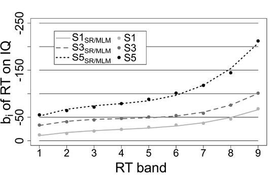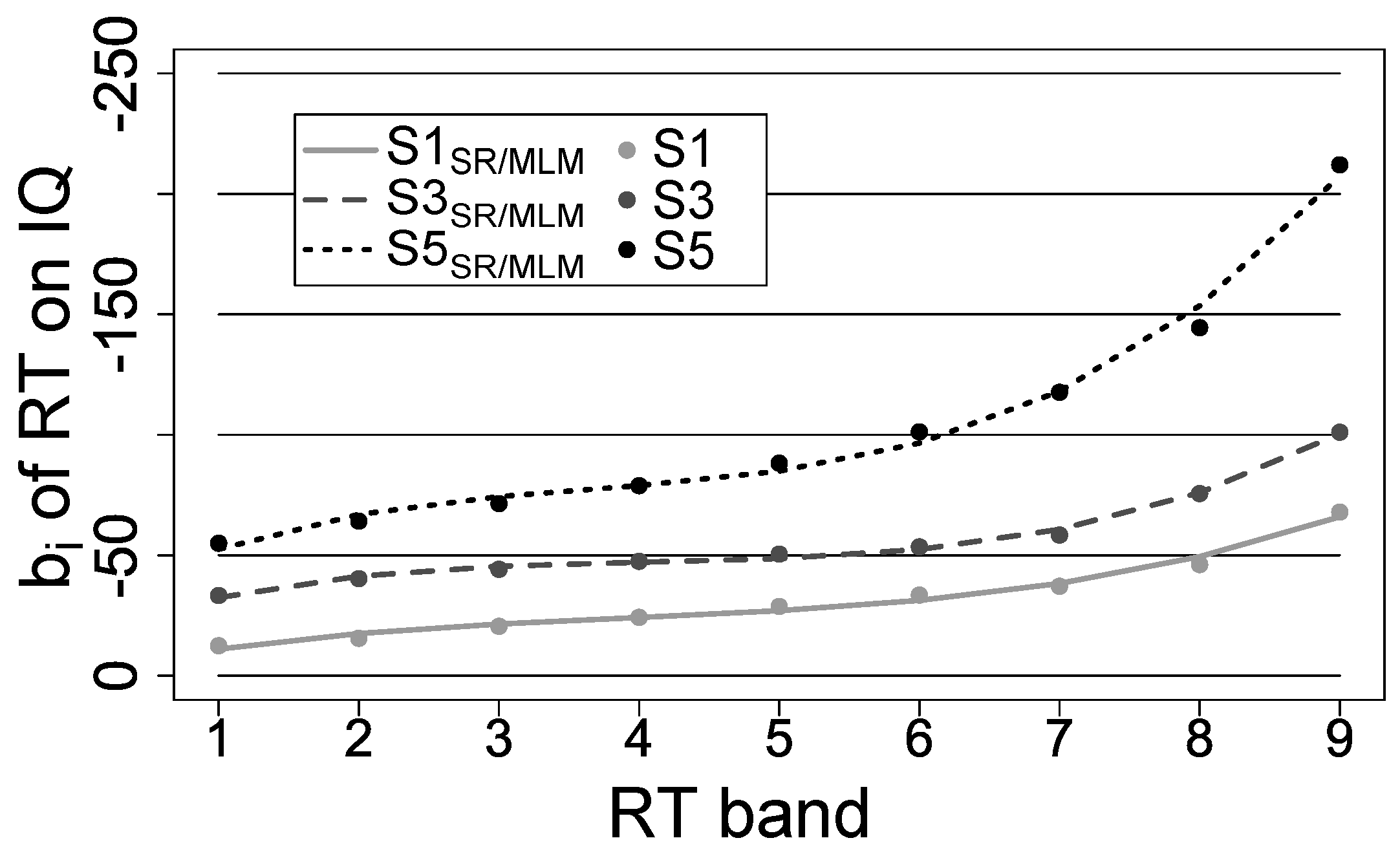In correspondence to the shape of increases of mean RT across performance bands (see Equation (4) in the section of the Multi-level approach), we implemented a polynomial function of third order. Not only does this function approximate the increases in unstandardized regression weights reasonably well ($R^2\ge .99$, see Figure 1, p. 12), but it also implements the moderation of the RT–g relationship by all performance band variables that describe the shape of increases in mean RT across performance bands (Equation (4)). This solution suited the present data very well. Beyond that, this may still be a good description for the WPR in performance measures that show normal distribution at the intra-individual level in general due to their characteristic shape of increases of mean performance across performance bands. Therefore, the second regression was specified as follows:

$$\begin{array}{c}\hfill b_B=b_L·B+b_Q·B^2+b_C·B^3+b_{00}+{ϵ}_b\end{array}$$

(2)

For this second regression, there are two parameters that quantify the significance and magnitude of the WPR. The variance explained by the regression (i.e., $R^2$) represents in how far the unstandardized regression weights increase across performance bands and thus the significance of the WPR. As a high $R^2$ only indicates how consistent the increases in unstandardized regression weights across RT bands are, an additional measure is needed to quantify the magnitude of the WPR.

The shape and magnitude of the increases across performance bands are determined by the size of the slope parameters within the regression ($b_L$, $b_Q$$b_C$)2. The intercept ($b_{00}$) of the regression represents the regression weight within the centred performance band (i.e., $B=0$). As the interpretation of the three slope parameters within this regression is rather complex, we propose a difference between $b_B$ in the worst performance (WP) percentile and in the best performance (BP) percentile in reference to mean performance ($M_{PF}$) as a measure for the effect size (ES) of the WPR:

$$\begin{array}{c}\hfill {\text{ES}}_{\text{WPR}}=\frac{b_{B\left(\text{WP}\right)}-b_{B\left(\text{BP}\right)}}{M_{PF}}\end{array}$$

(3)

This effect size basically corresponds to the effect size Cohen’s q comparing the correlation between best performance and g to the correlation between worst performance and g. It quantifies the magnitude of increase in unstandardized regression weights as percentage of mean performance in the respective task (for an example see p. 12). Still, it is a simplification with respect to the full shape of the increases in unstandardized regression weights across performance bands. As it does only reflect the absolute difference between best and worst performance bands, it does not represent the non-linear shape of increases between best and worst performance bands. Thus, increases in unstandardized regression weights should always be plotted by performance bands, so that the shape of increases can be evaluated as well. Nevertheless, the proposed effect size may be a good heuristic to evaluate in how far increases in unstandardized regression weights are larger in one task or condition compared to another.

Altogether, the sequential regression approach quantifies the WPR by predicting the magnitude of the relationship between g and performance across performance bands by band number. This provides a set of regression parameters that can be tested for statistical significance on the one hand, and an estimate for the consistency of increases across percentiles on the other hand.

Mutli-level moderation. The multi-level approach is essentially equal to the sequential regression approach, except it estimates all parameters of the sequential regression approach within one step. Accounting for the data structure of performance bands nested in participants, the multi-level approach combines Equations (1) and (2) by entering Equation (2) into Equation (1).

In addition, the intercept varies across performance bands for obvious reasons. The mean performance within each performance band evidently decreases with ascending performance bands. Specifically performance in the first band will be best or fastest, whereas performance in the last band will be worst or slowest. Therefore the intercept $b_0$ from Equation (1) should be able to change across performance bands as well.

Similar to the increase of unstandardized regression weights across performance bands, the intercept does not increase linearly across performance bands either. In fact, a linear increase of intercepts across performance bands would correspond to an equal distribution of performance at the intra-individual level. Usually we would assume intra-individual performance to be normally distributed, or in case of reaction times right-skewed (e.g., ex-Gaussian or Wald distributed). The intercepts within these distributions usually show non-linear increases across performance bands. These increases are again quite well approximated by a polynomial function of third order. For this, $b_0$ from Equation (1) will be predicted by percentile:

$$\begin{array}{c}\hfill b_{0B}=b_B·B+b_{B^2}·B^2+b_{B^3}·B^3+b_{B0}+{ϵ}_b\end{array}$$

(4)

Entering this equation into Equation (1) together with Equation (2) yields a prediction of the performance PF in each performance band B for participants i:

$$\begin{array}{cc}\hfill {\text{PF}}_{iB}& =(b_L·B+b_Q·B^2+b_C·B^3+b_{00})·g_i\hfill \\ \hfill & +(b_B·B+b_{B^2}·B^2+b_{B^3}·B^3+b_{B0})+{ϵ}_{iB}\hfill \end{array}$$

(5)

The term in the first line represents Equation (2) and the term in the second line represents Equation (4). Note that now performance within performance bands ${\text{PF}}_{iB}$ is the dependent variable and that all regression parameters are summarized within one Equation.

As multi-level modeling (MLM) allows to separate effects on level 1 (within a person) and level 2 (between people), we may additionally implement random effects for predictors on level 1. This means that the level 1 parameters (i.e., regression weights of performance bands) may vary across level 2 units (i.e., participants). Specifically, this reflects inter-individual differences in the increases of mean RT across performance bands that basically correspond to inter-individual differences in the intra-individual distribution of performance or RTs. This seemed reasonable to us and therefore the whole Equation (4) was estimated with random effects3. This results in a MLM equation with correct notation of:

$$\begin{array}{cc}\hfill {\text{PF}}_{iB}=& ({\gamma }_0+u_{i0})+({\gamma }_1+u_{i1})·B+({\gamma }_2+u_{i2})·B^2+({\gamma }_3+u_{i3})·B^3+\hfill \\ \hfill & {\gamma }_4·g_i+{\gamma }_5·(g_i\times B)+{\gamma }_6·(g_i\times B^2)+{\gamma }_7·(g_i\times B^3)+{ϵ}_{iB}\hfill \end{array}$$

(6)

The performance PF in each performance band B of each participant i is composed of a random intercept (${\gamma }_0+u_{i0}$) and random effects of performance band (${\gamma }_{1-3}+u_{i1-3}$). This first line of Equation (6) essentially is Equation (4) . Additionally, ${\text{PF}}_{iB}$ is predicted by a fixed effect of g (${\gamma }_4$), representing the relationship of ${\text{PF}}_{iB}$ and g for $B=0$ and cross level interactions between g and B (${\gamma }_{5-7}$), representing the increases of the relationship between ${\text{PF}}_{iB}$ and g across performance bands. This second line of Equation (6) basically represents Equation (2), with the difference that the interactions between performance band B and g are explicitly stated in Equation (6).

This Equation of the MLM allows to estimate the interaction between performance band and g on the relation between g and performance across performance bands. However, because the dependent variable within this approach is the performance within each performance band B, the overall explained variance $R^2$ of this regression does not refer to the same explained variance as in the second step of the sequential regression approach. In contrast, this approach treats the unstandardized regression weights between g and performance across performance bands as estimates, whereas the sequential regression approach enters these coefficients as manifest variables. Consequently, the sequential regression approach will underestimate the standard errors of coefficients in the second step and thus overestimates their statistical significance [22]. In this sense, the MLM approach results in more accurate estimates of the standard errors from a statistical perspective, because it does not underestimate the standard errors of the respective coefficients. Hence, the MLM approach judges the significance of coefficients more accurately than the sequential regression approach.

The interpretation of the results of the MLM approach is arguably more complex. There is no direct measure for the effect size of the WPR, because unlike the $R^2$ in the second step of the sequential regression approach, the $R^2$ of the MLM approach does not refer to the consistency of the increases of unstandardized regression weighs across performance bands. Instead it refers to the variance explained in the performance (${\text{PF}}_{iB}$) across performance bands. Still, the effect size introduced in Equation (3) can be computed in the MLM approach as well. For this, the unstandardized regression weight $b_B$ predicting PF by g across performance bands B can be estimated with ${\gamma }_4$ to ${\gamma }_7$:

$$\begin{array}{c}\hfill {\widehat{b}}_B={\gamma }_4+{\gamma }_5·P+{\gamma }_6·P^2+{\gamma }_7·P^3\end{array}$$

(7)

To calculate the effect size as stated in Equation (3) the regression weights for the best and worst performance bands can be estimated. The mean performance can be estimated with the fixed slope (${\gamma }_0$), when the performance band variable was centered. With these variables, the proposed effect size can then be calculated.

1.3.2. New WPA Approaches for Standardized Regression Weights

To implement these two WPA approaches on the level of standardized regression weights, the performance within each performance band has to be z-standardized on the inter-individual standard deviation (SD) of the respective performance band. Although we thereby lose information on the absolute increases in performance across performance bands (e.g., increasing RTs from best to worst performance bands) the covariance structure between performance across performance bands and g remains the same only that it is now controlled for increasing variances from best to worst performance. Furthermore, it is necessary that g is z-standardized for the analyses on the level of standardized estimates. However, we recommend to do that for both the analyses on the level of unstandardized and standardized estimates.

Sequential Regression. For the sequential regression approach with standardized estimates only the first step differs considerably from analysing unstandardized estimates. Specifically, we no longer predict the absolute performance PF of each participant i within each performance band B, but the z-standardized performance $z\left(\text{PF}\right)$ within each performance band B by general intelligence g:

$$\begin{array}{c}\hfill z\left({\text{PF}}_B\right)={\beta }_B·g+{ϵ}_i\end{array}$$

(8)

This results in standardized regression weights ${\beta }_B$ for each performance band quantifying the standardized relationship (i.e., correlation) between performance in each performance band with g. Please note that there is no longer any intercept for this regression, because the intercept is always zero when using z-standardized measures. The standardized regression weights across performance bands ${\beta }_B$ can again be predicted by the number of performance band in a second step that implements the moderation of the relationship between performance PF and g by performance band:

$$\begin{array}{c}\hfill {\beta }_B=b_L·B+b_{00}+{ϵ}_b\end{array}$$

(9)

According to the common assumption that correlations increase linearly from best to worst performance [3], we implemented only a linear increases in standardized regression weights across performance bands.4 Nevertheless, it is possible to implement non-linear increases in this approach as well. For this, additional regression weights specifying quadratic or cubic trends can be entered into Equation (9), just like in Equation (2).

Comparable to the sequential regression approach on the level of standardized regression weights, there are two parameters that quantify the significance of the WPR. On the one hand, the $R^2$ of this regression quantifies the consistency of increases in performance bands. On the other hand, the regression weight $b_L$ quantifies the size of increases across performance bands. The intercept $b_{00}$ quantifies the standardized relation for the centered performance band.

To quantify the magnitude of the WPR on the level of standardized estimates it is best to compute the effect size Cohen’s q from Equation (9). To do so, we calculate the estimated standardized regression weight for the best performance band ${\beta }_{\text{BP}}$ and the estimated standardized regression weight for the worst performance band ${\beta }_{\text{WP}}$. These can then be transformed into Z-values with a Fisher Z-transformation and the difference between $Z_{\text{WP}}$ and $Z_{\text{BP}}$ yields Cohen’s q [12].

Multi-level moderation. Again, the Multi-level approach is essentially equal to the sequential regression approach apart from the fact that it estimates both steps of the sequential regression approach in one step. For this, Equation (9) is entered into Equation (8), resulting in:

$$\begin{array}{cc}\hfill z\left({\text{PF}}_{iB}\right)& =(b_L·B+b_{00})·g+{ϵ}_{iB}\hfill \\ \hfill & =b_{00}·g+b_L·(B\times g)+{ϵ}_{iB}\hfill \end{array}$$

(10)

In contrast to the MLM approach on the level of unstandardized regression weights, it is not necessary to estimate a fixed effect of the increases in performance across performance bands (see Equation (4)), because the z-standardization of performance in each performance band resulted in a mean performance of zero within each performance band. However, a random effect for this effect can still be estimated. This effect reflects that there may not be full differential stability in performance across performance bands. For example, one person can show above average performance in best performance bands and only average performance in worst performance bands, whereas for another person the position in comparison to other participants stays the same across performance bands. This results in a full MLM equation with correct notation of:

$$\begin{array}{cc}\hfill z\left({\text{PF}}_{iB}\right)& ={\gamma }_1·g+{\gamma }_2·(B\times g)+({\gamma }_3+u_{i3})·B+{ϵ}_{iB}\hfill \end{array}$$

(11)

with the fixed effect ${\gamma }_3=0$ this results in:

$$\begin{array}{cc}\hfill z\left({\text{PF}}_{iB}\right)& ={\gamma }_1·g+{\gamma }_2·(B\times g)+\left(u_{i3}\right)·B+{ϵ}_{iB}\hfill \end{array}$$

Within this approach ${\gamma }_1$ represents the relationship between performance and g in the centred performance band and ${\gamma }_2$ represents the linear increase in this relationship across performance bands. The random effect $u_{i3}$ represents the variance in the relative position across performance bands for participants. In detail, this variance would be zero, if performance across performance bands is perfectly correlated.

As in the sequential regression approach, the increase in standardized regression weights can be computed with ${\gamma }_1$ and ${\gamma }_2$. Thus we can estimate the relationship between performance and g in the best and worst performance band and estimate the effect size Cohen’s q as difference between these two estimates on the level of Z-scores. Specifically, the estimated standardized regression weight within each performance band B can be estimated via:

$$\begin{array}{c}\hfill {\widehat{\beta }}_B={\gamma }_2·B+{\gamma }_1\end{array}$$

(12)

Once more, the MLM approach treats the standardized regression weights ${\beta }_B$ across performance bands as estimated, whereas the sequential regression approach treats them as manifest. Thus the MLM approach is generally, for unstandardized and standardized estimates, the statistically more sound approach because it will lead to less attenuated standard errors of increases in regression weights and thus does not inflate α-error probability of these increases.

1.4. Aims of the Empirical Example

The application of these newly introduced methods for WPA with empirical data has two main objectives. First, this will allow to compare the newly introduced methods for WPA to the traditional approach for WPA. Second, this comparison will allow to determine advantages and problems of the newly introduced methods, and may thereby convey which method and which level of analysis (unstandardized versus standardized) is adequate for a powerful analysis of the WPR.

Providing a powerful test and a quantification of the WPR would help researchers to determine processes that underlie the WPR and thus gain deeper knowledge on processes basic for g. Specifically, the newly introduced methods will not be capable of distinguishing between different theoretical explanations of the WPR. Nevertheless, they may present a more accurate analysis and test for the WPR and thereby provide researchers with a method that gives more robust results in studies that aim at testing different theoretical explanations of the WPR. This may help in finding processes underlying the WPR and result in a better understanding of processes fundamental to g.

To facilitate the use of the new approaches for WPA we provide commented R code for both approaches in the supplementary material. Additionally, the data of the empirical example are given in the supplementaries, so that the results can be reproduced and both approaches for unstandardized and standardized estimates can be studied in more detail.

2. Experimental Section

2.1. Participants

Data for this example were taken from a study over three measurement occasions with a cognitive abilities and personality assessment on the second measurement occasion. For this study, 134 participants from the area around Heidelberg, Germany were recruited. Participants’ age ranged from 18 to 61 years (M${}_{age}$ = 37.12, SD${}_{age}$ = 13.75), 60.4% were female, and they had different educational and occupational backgrounds.

For the present analysis we used data from the first and second measurement occasion. Some participants dropped out and one participant was excluded due to extreme scores (for a detailed description of the outlier analysis see the statistical analyses section on page 10). This resulted in a sample of 121 participants (58.7% female) aged from 18 to 61 years (M${}_{age}$ = 36.64, SD${}_{age}$ = 15.65) that were included in this analysis.

2.2. Measures

Sternberg Memory Span Task. The cognitive processing task analyzed in the present study was a computerized version of the Sternberg Memory Span Task [29] also used by Schubert et al. [2]. In this task participants were shown a memory set consisting of one to five numbers from 0 to 9 on a black computer screen. Subsequently, participants were shown a probe number and had to decide whether the probe was or was not contained in the afore presented number set by pressing one of two keys. The position of keys indicating whether the probe item was part of the memory set or not was counterbalanced across participants.

Three experimental conditions with different memory set sizes (1, 3, and 5 numbers) were administered. All three blocks started with ten practice trials with feedback, followed by 100 test trials without feedback. The order of the three memory set size conditions was counterbalanced across participants. Between blocks participants were offered a short break.

Each trial started with a fixation cross presented for 1000 to 1500 ms. Then, numbers were presented sequentially for 1000 ms. Between numbers a blank screen was presented for 400 to 600 ms. After the last number of the memory set was presented, a black screen with a question mark was shown for 1800 to 2200 ms, followed by a probe item showing a single digit. Participants then had to indicate whether the number was part of the memory set or not by pressing the corresponding key on a standard computer keyboard.5 After the response the probe item remained on screen for 1000 ms, followed by an inter-trial interval of 1000 to 1500 ms. The stimuli were presented on a 17 inch LED computer screen and the experiment was programmed in E-Prime 2.0 Professional.

Berlin Intelligence Structure Test (BIS). Within the cognitive abilities and personality assessment, participants completed the Berlin Intelligence Structure Test (BIS [30]). The assessment was carried out according to the standardized instructions. The assessment ran in groups of up to four persons and started with the BIS assessment, followed by a personality questionnaire (NEO-FFI), the Raven Advanced Progressive Matrices, and a demographic questionnaire. For this study only the BIS results were analyzed.6

BIS results were evaluated in correspondence with the evaluation instructions from the manual. First, raw scores were determined for all tasks and subsequently the raw scores were transformed into standardized scores. From these scores one score for general intelligence (g) was calculated.

2.3. Statistical Analyses

Outlier Analysis. Before running all analyses, we carefully examined the data for uni- and multivariate outliers in a three-step procedure. First we discarded all RTs with incorrect responses. For all correct response RTs we checked for intra-individual outliers in reaction times: initially, reaction times lower than 100 ms and higher than 3000 ms were excluded for all participants. Then, we computed mean and standard deviation for the logarithmized reaction time within each participant and each experimental condition, and excluded reaction times below and above three standard deviations from the mean of logarithmized reaction times.

Secondly, participants with univariate outliers in reaction time and intelligence test scores were excluded from the data analysis when mean reaction time or intelligence test scores showed an absolute difference larger than three standard deviations from the sample mean. Finally, multivariate outliers on the combination of mean RT in each condition and intelligence test score were excluded when they had a Mahalanobis distance larger than 13.816, corresponding to ${\chi }^2{\left(2\right)}_{p<.001}$. In an iterative process, this procedure was repeated until no further participants were detected as multivariate outliers. Within this procedure, one person was identified as a uni-variate outlier on general intelligence, processing speed, creativity, and verbal abilities ($z_s<-3)$, as well as a multivariate outlier on the combination of IQ and RT in experimental conditions with memory set size 1 and 5 (Mahalanobis Distance = 14.08–16.71).

Statistical Analysis. Both the sequential regression approach and the MLM approach were calculated with R [32] and conducted separately for the three experimental conditions of the Sternberg memory span task. For the sequential regression analysis, regressions were estimated in a stepwise procedure. First, performance within each RT band was predicted by general intelligence (see Equations (1) and (8)), and second, the unstandardized and standardized regression weights from step one were predicted by RT band (see Equations (2) and (9)).

The analysis of the MLM approach of the Worst Performance Rule was conducted using the nlme package in R [33]. In a stepwise procedure all parameters from Equations (6) and (11) were added to a Random Intercept Model that served as baseline model. As following models were nested, models with additional parameters were required to show significant increase in Log likelihood to be considered a better data description. In addition, decreases in Akaike’s Information Criterion (AIC) and Bayesian Information Criterion (BIC) were used as indicators for model fit.

Fixed effects were tested for significant deviation from zero using a one-sided t-test. Further, random slopes were tested for significance with a Likelihood-Ratio test. Additionally, random effects were estimated with an unstructured G-Matrix, not only estimating the variances of each random effect but additionally estimating the covariances between all random effects.

For both approaches, nine RT bands that contained 9 to 11 RTs were constructed, so that each RT band contained approximately 11.1% of RTs of the intra-individual RT distribution. Although many other studies used percentiles or RT bands with five RTs in each band, we decided to construct nine RT bands in order to be able to center the RT band variable to a meaningful value (i.e., the fifth RT band). If two reaction times at the border of an RT band were equal, they were assigned to different RT bands. RT band number (i.e., performance band variable B) was centered to the fifth RT band of the intra-individual RT distribution, in order to obtain meaningfully interpretable estimates for the fixed intercepts and fixed slopes [28]. Specifically, the intercept represents approximately the median RT of an average intelligent person and the fixed effect of g represents the unstandardized regression weight from g on RT in the fifth RT band. After centering B to the fifth RT band, $B^2$ and $B^3$ were derived from the centred B-variable. The general intelligence score (g) from the BIS was z-standardized within the sample.

3. Results and Discussion

3.1. Descriptives

Descriptive statistics for the Sternberg memory span task and BIS results are given in

Table 1. Descriptives for the Sternberg Task and the BIS.

Measure	Mean	Median	SD	Min	Max	Rel.
S1 (RT)	587.9	564.8	111.0	396.2	969.5	.96 ${}^{\mathrm{a}}$
S3 (RT)	726.7	694.0	166.8	479.0	1372.0	.98 ${}^{\mathrm{a}}$
S5 (RT)	889.6	828.0	241.7	539.4	1638.0	.97 ${}^{\mathrm{a}}$
BIS ${}^{\mathrm{c}}$	99.6	99.7	5.7	86.3	114.8	.94 ${}^{\mathrm{b}}$

Note: Rel. = reliability; ${}^{\mathrm{a}}$ Estimated via Odd-Even correlations—for this trials were separated into odd and even trials by trial-number; ${}^{\mathrm{b}}$ Estimated via Cronbach’s α; ${}^{\mathrm{c}}$ Standardized scores of the BIS are set to have a mean of 100 and a standard deviation of 10.

. In line with earlier results, RT increased with larger memory set size, $F(2,240)=277.5$, $p<.05$, $ϵ=.69$, ${\omega }^2=.70$. The BIS scores were representative compared to the standardization sample, $t\left(120\right)=-.71$, $p>.05$, Cohen’s $d=-.06$.7 There were no significant differences in general intelligence between women and men, $t\left(119\right)=.95$, $p>.05$, Cohen’s $d=.18$.

3.2. Results from New WPA Approaches with Unstandardized Regression Weights

3.2.1. Results of the Sequential Regression Approach

In the first step of the sequential regression approach, general intelligence predicted reaction time within RT bands across all three conditions, $F\mathrm{s}(1,119)\ge 6.7$, $p\mathrm{s}<.05$ and $R^2\mathrm{s}=$ .05–.22. Specifically, these results convey that inter-individual differences in mean reaction time in each RT band across all three conditions were predicted by general intelligence. In the second step, the number of RT band predicted the unstandardized regression weights across RT bands in all three conditions, $F\mathrm{s}(3,5)\ge 127.2$, $p\mathrm{s}<.05$ and $R^2\mathrm{s}\ge .98$ (for an illustration of the regressions estimated in the second step, see Figure 1).

All estimated parameters differed significantly from zero (see

Table 2. Estimated parameters for the sequential regression approach with unstandardized regression weights.

Parameters		Condition
		S1		S3		S5
		Estimate	S.E.	Estimate	S.E.	Estimate	S.E.
$b_{00}$	(Int.)	−27.00 *	1.25	−48.62 *	0.85	−84.93 *	2.86
$b_{WPR1}$	(B)	−3.32 *	0.84	−2.26 *	0.57	−8.11 *	1.92
$b_{WPR2}$	($B^2$)	−0.72 *	0.14	−1.11 *	0.10	−2.81 *	0.32
$b_{WPR3}$	($B^3$)	−0.22 *	0.07	−0.39 *	0.04	−0.70 *	0.15
$R^2$		.98		1.00		.99

Note: S.E. = standard error of the respective estimate; * Indicates p < .05; The terms in brackets indicted the predictor corresponding to the respective parameter.

). As indicated by the effect size proposed in Equation (3), increases in the unstandardized regression weight $b_B$ did not differ between set size 1 and 3, but tended to be larger for set size 5 (${\text{ES}}_{S1}=.09$, ${\text{ES}}_{S3}=.09$ and ${\text{ES}}_{S5}=.17$). Specifically, this means that the increases in the unstandardized regression weight from best to worst performance correspond to 9% to 17% of the mean reaction time in the corresponding condition. For example, in the S1 condition the mean performance was 587.9 ms. With an ES = .09, the difference of the unstandardized regression weight between best and worst performance thus was about 52.9 ms. This means that the difference in RT between an individual one SD above average in IQ and an individual average in IQ increased for 52.9 ms from best to worst performance RT band.

3.2.2. Results of the MLM Approach

For all three conditions the Log-likelihood (LL) ratio tests indicated best fit for the full MLM with all parameters included (see

Table 3. Estimates for model fit of the MLM across all three conditions for the WPA with unstandardized regression weights.

Cond	Model		DF	AIC	BIC	LogLik	L. Ratio	p
S1	Base		3	14,352.4	14,367.3	−7173.2	–	–
	1	($+{\gamma }_1$)	4	13,099.3	13,119.2	−6545.6	1255.1	.000
	2	($+{\gamma }_2$)	5	12,891.7	12,916.7	−6440.8	209.6	.000
	3	($+{\gamma }_3$)	6	12,775.8	12,805.8	−6381.9	117.9	.000
	4	($+u_{i1}$)	8	11,657.3	11,697.2	−5820.6	1122.6	.000
	5	($+u_{i2}$)	11	11,247.5	11,302.4	−5612.7	415.8	.000
	6	($+u_{i3}$)	15	10,940.2	11,015.1	−5455.1	315.3	.000
	7	($+{\gamma }_4$)	16	10,939.3	11,019.2	−5453.6	2.9	.090
	8	($+{\gamma }_5$)	17	10,937.7	11,022.6	−5451.9	3.6	.059
	9	($+{\gamma }_6$)	18	10,938.9	11,028.8	−5451.5	0.8	.369
	10	($+{\gamma }_7$)	19	10,937.0	11031.9	−5449.5	3.9	.049
S3	Base		3	14,825.1	14,840.1	−7409.5	–	–
	1	($+{\gamma }_1$)	4	13,630.7	13,650.6	−6811.3	1196.4	.000
	2	($+{\gamma }_2$)	5	13,465.1	13,490.1	−6727.6	167.6	.000
	3	($+{\gamma }_3$)	6	13,343.2	13,373.2	−6665.6	123.9	.000
	4	($+u_{i1}$)	8	12,329.8	12,369.7	−6156.9	1017.4	.000
	5	($+u_{i2}$)	11	11,736.6	11,791.5	−5857.3	599.2	.000
	6	($+u_{i3}$)	15	11,260.5	11,335.4	−5615.2	484.2	.000
	7	($+{\gamma }_4$)	16	11,255.3	11,335.2	−5611.6	7.2	.007
	8	($+{\gamma }_5$)	17	11,255.9	11,340.8	−5610.9	1.4	.236
	9	($+{\gamma }_6$)	18	11,257.8	11,347.7	−5610.9	0.0	.847
	10	($+{\gamma }_7$)	19	11,253.2	11,348.1	−5607.6	6.7	.010
S5	Base		3	15,501.8	15,516.8	−7747.9	–	–
	1	($+{\gamma }_1$)	4	14,245.4	14,265.4	−7118.7	1258.4	.000
	2	($+{\gamma }_2$)	5	14,038.7	14,063.7	−7014.4	208.7	.000
	3	($+{\gamma }_3$)	6	13,905.5	13,935.5	−6946.8	135.2	.000
	4	($+u_{i1}$)	8	12,740.3	12,780.2	−6362.1	1169.3	.000
	5	($+u_{i2}$)	11	12,265.7	12,320.6	−6121.9	480.6	.000
	6	($+u_{i3}$)	15	11,974.5	12,049.4	−5972.3	299.2	.000
	7	($+{\gamma }_4$)	16	11,971.0	12,050.9	−5969.5	5.5	.019
	8	($+{\gamma }_5$)	17	11,970.6	12,055.4	−5968.3	2.4	.119
	9	($+{\gamma }_6$)	18	11,965.3	12,055.1	−5964.6	7.3	.007
	10	($+{\gamma }_7$)	19	11,948.5	12,043.4	−5955.3	18.8	.000

Note: Cond = condition, LogLik = Log Likelihood, L. Ratio = Log Likelihood Ratio in comparison to the model one line above, Base = Baseline model, Expressions in parentheses denote variables added to the model.

). Although successive LL-ratio tests did not always indicate significant improvement in fit, for S1, the comparison of model 6 to 10 showed improved model fit, ${\chi }^2\left(4\right)=11.1$, $p<.05$, for S3, the comparison of model 7 to 10 indicated improved model fit, ${\chi }^2\left(3\right)=8.1$, $p<.05$, and for S5, the comparison of model 7 to 10 indicated better model fit, ${\chi }^2\left(3\right)=28.5$, $p<.05$ (see Table 3).

The AIC decreased across successive models, except within the S3 conditions for models 7 to 9. For models 6 to 10 in the S1 and S3 conditions, these decreases were below the critical difference of 10, which is often used as a cut off criterion for significant differences in model fit [34]. The BIC indicated best fit for the full MLM only in the S5 condition. For S1, the BIC was lowest for model 6, without the prediction of ${\text{PF}}_{iB}$ by g and interactions between RT band and g (i.e., without ${\gamma }_4$ to ${\gamma }_7$). And for S3, BIC was lowest for model 7, without interactions between RT band and g (i.e., without ${\gamma }_5$ to ${\gamma }_7$). However, as the prediction of ${\text{PF}}_{iB}$ by g and interactions of g with RT band were the core of the present analysis and because the LL-ratio tests for model fit indicated better fit for the more complex models, we retained the full MLM for all three conditions.

The parameters estimating the WPR from the retained MLMs were numerically equivalent to those from the sequential regression approach (see

Table 4. Parameters estimating the WPR within the MLM approach with unstandardized regression weights.

Parameters		Condition
		S1		S3		S5
		Estimate	S.E.	Estimate	S.E.	Estimate	S.E.
${\gamma }_4$	(g)	−27.00 *	8.79	−48.62 *	12.02	−84.93 *	18.4
${\gamma }_5$	($g\times P$)	−3.32 *	1.42	−2.26	1.30	−8.11 *	2.53
${\gamma }_6$	($g\times P^2$)	−0.72 *	0.34	−1.11 *	0.51	−2.81 *	0.53
${\gamma }_7$	($g\times P^3$)	−0.22 *	0.11	−0.39 *	0.15	−0.70 *	0.16

Note: S.E. = standard error of the respective parameter; * Indicates p < .05; The expression in brackets indicates the predictor corresponding to each parameter.

). All other parameters for the MLMs in all three conditions can be reproduced with the syntax and data given in the supplementary material online. As parameters from the MLM were equal to the parameters from the sequential regression approach, the estimated effect sizes were equal for the MLM likewise (${\text{ES}}_{S1}=.09$, ${\text{ES}}_{S3}=.09$ and ${\text{ES}}_{S5}=.17$).

The standard errors for the coefficients were considerably larger in the MLM than in the sequential regression approach. As mentioned earlier, this is because the MLM approach treats the covariances between ${\text{PF}}_{iB}$ and g across RT bands as estimated, whereas the sequential regression approach treats them as observed. Thus, the sequential regression approach underestimates the standard errors of the coefficient and the MLM approach estimates the standard errors more accurately (see p. 7). This is why one parameter (${\gamma }_5$) in the S3 condition did not differ from zero to a statistically meaningful extent in the MLM approach, although parameters showed significant differences from zero in the sequential regression approach.

Altogether, these results showed that both approaches, the sequential regression approach and the MLM approach, estimate the WPR via an interaction between RT band and g. In addition to RT band and g itself, this interaction predicts the performance in each RT band. Beyond that, results showed that increases in unstandardized regression weights between performance in each RT band and g are almost perfectly predicted by RT band ($R^2\ge .99$).

3.3. Results from New WPA Approaches with Standardized Regression Weights

3.3.1. Sequential Regression Approach

On the level of standardized regression weights, in step one, z-standardized RT was predicted by g across all performance bands in all three experimental conditions, $F_{\mathrm{s}}(1,119)\ge 6.7$, $p_{\mathrm{s}}<.05$, and $R^2$ = .05–.22. In step two, results showed that standardized regression weights ${\beta }_B$ increased in absolute size in the S1 and S5 condition, whereas standardized regression weights decreases in size in the S3 condition (see

Table 5. Estimated parameters from WPA with z-standardized RTs as DVs.

Condition	Parameter		Seq. Regression		MLM
	Seq. Reg.	MLM	Estimate	S.E.	Estimate	S.E.
S1	$b_{00}$	${\gamma }_1$	−.266 *	.004	−.266 *	.082
	$b_L$	${\gamma }_2$	−.006 *	.001	−.006	.010
S3	$b_{00}$	${\gamma }_1$	−.336 *	.005	−.336 *	.083
	$b_L$	${\gamma }_2$	.008 *	.001	.008	.007
S5	$b_{00}$	${\gamma }_1$	−.409 *	.005	−.409 *	.081
	$b_L$	${\gamma }_2$	−.008 *	.002	−.008	.007

Note: Seq. Regression and Seq. Reg. = sequential regression approach; S.E. = standard error of the respective parameter; * Indicates p < .05.

for the estimated parameters). Additionally, the results from step two showed that standardized regression weights were overall smallest in the S1 condition and increased with larger memory set size, which is reflected in increasing size of the intercepts from S1 to S5 (see Table 5).

With respect to the consistency and magnitude of increases across RT bands, the results from the sequential regression with standardized estimates suggested that increases of standardized regression weights across RT bands were less consistent, $R^2=$ .66–.67, than increases of unstandardized regression weights. Furthermore, the magnitude of increases was slightly smaller in the S1 condition ($q=.05$) than in the S5 condition ($q=.08$). In the S3 condition standardized regression weights actually decreased in size from best to worst performance bands ($q=-.07$). Thus, the S3 condition contradicted the WPR on the level of standardized regression weights.

3.3.2. MLM Approach

For all three conditions, the Log-likelihood-ratio tests indicated best model fit for a MLM model without the interaction of $g\times B$ (i.e., model 2), indicating that there are no increases in the relationship between g and RT across RT bands (see

Table 6. Estimates for model fit of the MLM with standardized regression weights across all three conditions.

Cond	Model		DF	AIC	BIC	LogLik	L. Ratio	p
S1	Base		3	1313.0	1328.0	−653.5	–	–
	1	($+u_{i3}$)	5	384.1	409.0	−187.0	933.0	.000
	2	($+{\gamma }_1$)	6	376.0	406.0	−182.0	10.0	.000
	3	($+{\gamma }_2$)	7	377.7	412.6	−181.8	0.4	.551
S3	Base		3	588.2	603.2	−291.1	–	–
	1	($+u_{i3}$)	5	−399.1	−374.2	204.6	991.3	.000
	2	($+{\gamma }_1$)	6	−412.5	−382.6	212.3	15.4	.000
	3	($+{\gamma }_2$)	7	−411.7	−376.7	212.8	1.1	.287
S5	Base		3	534.5	549.5	−264.2	–	–
	1	($+u_{i3}$)	5	−297.4	−272.5	153.7	835.9	.000
	2	($+{\gamma }_1$)	6	−319.5	−289.6	165.8	24.1	.000
	3	($+{\gamma }_2$)	7	−318.8	−283.9	166.4	1.3	.249

Note: Cond = condition, LogLik = Log Likelihood, L. Ratio = Log Likelihood Ratio in comparison to the model one line above, Base = Baseline model, Expressions in parentheses denote the variable added to the model.

for model fit). AIC and BIC likewise indicated best model fit for a MLM model without the interaction of $g\times B$, although $\Delta \text{AIC}$ is below the critical value of 10 in the S1 condition and $\Delta \text{BIC}$ is below the critical value of 10 for the S1 and S3 condition. Altogether these results indicate that there are significant relationships between g and RT, however this relationship does not vary across RT bands, contrary to the predictions made by the WPR.

However, if we take a look at the estimated parameters of model 3 with the interaction of $g\times B$ (see Table 5), the results show that the numerical estimates for the relationship in $B=0$ between g and RT (i.e., $b_{00}$ or ${\gamma }_1$) and the increases across RT bands (i.e., $b_L$ or ${\gamma }_2$) are equal for the sequential regression approach and the MLM approach in all three conditions. The difference in the significance of these parameters is again due to larger standard errors in the MLM approach. Just as in the analyses with unstandardized regression weights, this can be explained by the fact that the sequential regression approach treats the standardized regression weights across RT bands as manifest and the MLM approach treats them as estimated. Thus, the MLM approach takes into account that there is uncertainty in the estimation of standardized regression weights across RT bands and estimates standard errors of the parameters accordingly. All in all, the MLM approach is therefore more accurate and the results suggest that there is no WPR on the level of standardized regression weights.

3.4. Results from a Traditional WPA

To compare the results of the two introduced methods with results from a traditional worst performance analysis, we performed the latter as well. For this, we calculated mean RTs for the 9 RT bands within each participant in all experimental conditions. Then, we computed correlations of the mean RTs across RT bands with the BIS score.

For the S1 and S5 condition, the WPR was replicated with slightly more consistently increasing correlations across RT bands in the S5 condition (see

Table 7. Covariance, unstandardized regression weight, standard of RT, correlation, and reliability of RTs across the nine RT bands in all three experimental conditions.

P	S1					S3					S5
	Cov	$b_{RT,g}$	${SD}_{RT}$	$r_{RT,g}$	Rel.	Cov	$b_{RT,g}$	${SD}_{RT}$	$r_{RT,g}$	Rel.	Cov	$b_{RT,g}$	${SD}_{RT}$	$r_{RT,g}$	Rel.
1	−12.4	−12.4	51.5	−0.24	.98	−33.3	−33.3	96.1	−0.35	.99	−55.0	−55.0	140.5	−0.39	.99
2	−15.5	−15.5	67.3	−0.23	1.00	−40.3	−40.3	111.7	−0.36	1.00	−64.1	−64.1	164.2	−0.39	1.00
3	−20.5	−20.5	80.1	−0.26	1.00	−44.2	−44.2	121.8	−0.36	1.00	−71.4	−71.4	179.3	−0.40	1.00
4	−24.2	−24.2	91.6	−0.26	1.00	−47.5	−47.5	134.4	−0.35	1.00	−78.9	−78.9	201.2	−0.39	1.00
5	−28.8	−28.8	103.0	−0.28	1.00	−50.5	−50.5	146.8	−0.34	1.00	−88.2	−88.2	221.8	−0.40	1.00
6	−33.5	−33.5	116.4	−0.29	1.00	−53.5	−53.5	163.3	−0.33	1.00	−101.2	−101.2	251.0	−0.40	1.00
7	−37.1	−37.1	135.2	−0.27	1.00	−58.4	−58.4	183.2	−0.32	1.00	−117.7	−117.7	283.8	−0.41	1.00
8	−46.1	−46.1	161.4	−0.29	1.00	−75.6	−75.6	228.5	−0.33	1.00	−144.5	−144.5	336.0	−0.43	1.00
9	−67.9	−67.9	245.3	−0.28	.96	−101.1	−101.1	355.7	−0.28	.98	−212.1	−212.1	454.4	−0.47	.98
R		−1.00	1.00	−.82			−1.00	1.00	.90			−1.00	1.00	−.91

Note: P = number of RT band, Cov = covariance between RT and g, $b_{RT,g}$ = unstandardized regression weight predicting RT by g, $S{D}_{RT}$ = inter-individual standard deviation of mean RT within each RT band, $r_{RT,g}$ = correlation between RT and g, Rel. = reliability of RT estimated with odd-even correlations—for this Trials were separated into odd and even trials by trial number and reliability of all RT in an performance band was estimated with the Spearman-Brown formula, R = Spearman’s rank correlation between RT band and the variable presented in the column.

). Furthermore, the effect size Cohen’s q for the difference between correlations in best and worst performance RT band was higher in the S5 condition ($q_{S5}=.10$) than in the S1 condition ($q_{S1}=.04$). In the S3 condition, correlations were positively associated with RT band number and decreased in absolute value with ascending RT bands. The S3 condition thus did not replicate the WPR. However, the differences in correlations between best and worst performance bands did not differ significantly from zero for all three conditions, $Z_{S1}=.41,p=.68$, $Z_{S3}=-1.08,p=.28$, and $Z_{S5}=1.47,p=.14$.

The estimated reliability for RTs within RT bands was high across all RT bands and conditions (see Table 7). Since reliabilities did not increase with ascending RT bands, the increases in correlations between RT and g cannot be attributed to decreases in error variance with ascending RT bands.

Altogether, the results from a traditional WPA differed from the results of the sequential regression and the MLM approach with unstandardized regression weights. Although there were consistent increases in correlations across RT bands in the S1 and S5 condition (Spearman’s rank correlation $r=-.82$ to $-.91$) suggesting a WPR, the size of the differences in correlations across RT bands was not significant. Thus the traditional WPA described the WPR, but the actual test for increases in correlations across RT bands was not significant in all three experimental conditions. The results from the MLM approach with standardized regression weights were in line with the results from the z-Test and indicated that there is no WPR. Considering that the sequential regression approach with standardized regression weights estimated equal parameters as in the MLM approach but overestimates the significance of these parameters, the results of the sequential regression approach with standardized regression weights may be interpreted the same way.

In contrast, both the sequential regression approach and the MLM approach on the level of unstandardized regression weights showed significant increases in unstandardized regression weights from best to worst performance bands in all three conditions that support the WPR. On the one hand, the consistency of increases in unstandardized regression weights analyzed in the sequential regression approach and in the MLM approach was substantially larger ($R^2\ge$ .99) than in the analysis of correlations in the traditional WPA and of standardized regression weights ($R^2$ = .66 to .83). On the other hand, on the level of unstandardized regression weights the increases were all consistent with the WPR, whereas on the level of standardized regression weights and correlations there was a decrease in the size of correlations with ascending RT bands in the S3 condition. All in all, there are considerable differences between results on the level of unstandardized versus standardized regression weights that need to be discussed.

3.5. Discussion

The present work conceptualized the WPR as a moderated effect of g on performance in a cognitive processing task that depends on the performance band or percentile in which performace is measured. Following this idea, we introduced two approaches to analyze the WPR. Both approaches were tested on the level of unstandardized and standardized estimates in an empirical example. unstandardized regression weights quantifying the relation between g and RT across RT bands showed perfect monothonic increases from best to worst performance bands. In correspondence to a larger WPR in tasks with higher g-loadings [3,17], the increases tended to be larger in more complex conditions. However, comparing the results with unstandardized regression weights to results with standardized regression weights and to results from a traditional WPA showed that increases in unstandardized regression weights do not necessarily correspond to the WPR from a traditional WPA perspective.

3.5.1. Differences in Analyses with Unstandardized and Standardized Estimates

These differences between results with unstandardized regression weights and results with standardized regression weights or results from traditional WPA are due to increases in inter-individual standard deviation of RT across performance bands. Equally to the covariance, the inter-individual standard deviation of RT ($S{D}_{RT}$) increased consistently (Spearman’s rank correlation: $r=1.00$) from best to worst performance bands (see Table 7). Furthermore, for a pair of highly correlated variables (e.g., $R{T}_{BP}$ and $R{T}_{WP}$) with different variances, the covariance between these two variables and a third variable g increases proportionally to the increase in variance. As correlations between mean RT across performance bands are medium to very high ($r=.55$ to $.99$ for the present sample), it may be that larger standard deviations of RT in worst performance percentiles lead to higher covariances with g, given that the covariance with g is a function of the variance for perfectly correlated variables. If this were the case, the increase in unstandardized regression coefficients that basically represents the covariance may be nothing else but a reflection of the increase in inter-individual standard deviation of RT. It seems that this was exactly the case in the present study, because analyses on the level of standardized regression weights that control for increases in variance across performance bands did not show the WPR.

In contrast to Coyle [3] who stated that differences in variance between best and worst performance do not affect the WPR, the present results show that increases in variance from best to worst performance may play a crucial role for the WPR, especially if best and worst performance is highly correlated. Specifically, the WPR on the level of correlations relies on increases in covariance between performance and g from best to worst performance that are proportionally larger than and independent from increases in variance in performance from best to worst performance bands. Despite the fact that results of analyses on the level of standardized regression weights may provide the actual WPR, we think that it is noteworthy that variance as well as covariance with g in worst performance band is notably larger than in best performance bands. In a nutshell, there are larger inter-individual differences in worst performance RT than in best performance RT that may drive the increase in covariance with g from best to worst performance bands. It would be interesting to see in how far this result is present in other basic cognitive processing task as well.

3.5.2. Differences between Newly Introduced WPA and Traditional WPA

Beyond the difference in analyses with unstandardized and standardized regression weights, there are important differences between traditional WPA and the newly introduced methods to analyze the WPR. Specifically, the traditional WPA described the increases in correlations accross RT bands, whereas the newly introduced methods provided an acutal test and a quantification for the magnitude of the WPR. Although the consistency and significance of increases in correlations across RT bands was sometimes tested with Spearman’s rank-correlations or a Fisher’s Z-Test [10], this is not sufficient for quantifying the actual magnitude and shape of increases across RT bands. Despite the possibility to compute an effect size for the difference in correlations across RT bands (Cohen’s q) as a measure fot the magnitude of the WPR, a test for the significance of these differences lacks statistical power [12]. By modelling the increases in unstandardized and standardized regression weights as a moderation, the newly introduced methods provided an actual test for the significance of the WPR and a quantification for the magnitude of the WPR. Furthermore, the newly introduced methods take the full shape of increases in unstandardized or standardized regression weights across all performance bands into account, whereas the Z-test only evaluates in how far correlations from best to worst performance with g differ significantly. And additionally, the test for consistency in increases across performance bands with Spearman’s rank correlations is flawed like the sequential regression approach, because it treats the estimated correlations in performance bands as manifest and does not account for the error in estimation. Altogether, the new methods thus overcome some major problems of traditional WPA.

3.5.3. Discussion of Differences between the Sequential Regression and the MLM Approach

With respect to differences between the two newly introduced methods, the results showed that the coefficients estimated to describe the increases in unstandardized and standardized regression weights are equal for both approaches. However, the standard errors of these coefficients were smaller for the sequential regression approach than for the MLM approach. Although smaller standard errors may seem as an advantage of the sequential regression approach, this approach actually underestimates the standard errors because the unstandardized regression weights across RT bands analyzed in the second step are treated as observed [22]. This leads to an overestimation of the significance, and thus may in turn provide an overly liberal judgement regarding the significance of the WPR. In contrast, the MLM approach treats the unstandardized regression weights across RT bands as estimated and thus provides unbiased standard errors. Taken together, the MLM approach is the more accurate method to analyze the WPR on the level of unstandardized and standardized regression weights. Therefore, we strongly recommend using the MLM approach instead of the sequential regression approach, because the sequential regression approach has serious shortcomings from a statistical perspective.

4. Conclusions

All in all, conceptualizing the WPR as moderation of the effect of g on RT by RT band not only allowed to test the WPR but also provided a quantification of the WPR. We thereby introduced a new way of analyzing the WPR that may overcome the problem of weak power when testing the difference of two correlations, takes the whole shape of increases of unstandardized or standardized estimates across performance bands into account, and additionally quantifies the increases of unstandardized and standardized regression weights across RT bands.

These newly introduced methods for analyzing the WPR suggested that there are perfectly consistent increases in unstandardized regression weights across RT bands in all three experimental conditions. The differences between traditional WPA and results with standardized regression weights to the results with unstandardized regression weights are driven by variations in inter-individual standard deviation of performance across RT bands. And finally, the interaction between RT band and g additionally suggests that general intelligence is related to the shape of the intra-individual performance distribution and not only to the mean performance.

Although these results give promising new insights on the WPR, further evidence with the newly introduced methods with larger sample sizes is needed. Especially because the estimation of the MLM approach is complex and robust estimates of the cross-level interactions can only be obtain in sufficiently large samples. Nonetheless, these results provide preliminary evidence for the feasibility of the newly introduced methods and therefore we hope that researchers will adopt these methods in future studies to gain deeper knowledge of the WPR and its underlying processes.

Nevertheless, by reformulating the WPR in regression termini the two new methods have provided a tool for more sophisticated analyses in future research that aims at an explanation of the WPR. The most accurate method to analyze the WPR would be the MLM approach. Although the sequential regression approach provides equal estimates for the actual increases of unstandardized and standardized regression weights and may be more accessible to use, researchers should bear in mind that the sequential regression approach overestimates the significance of these increases. Therefore, we advise researchers to use the MLM approach and otherwise discuss results from the sequential regression approach reluctantly.

Finally, analyzing the WPR on the level of unstandardized regression weights showed that other context variables, such as the inter-individual standard deviation of performance within each RT band, may affect the results when investigating the WPR on the level of correlations. Therefore future studies should consider analyzing the WPR on the level of unstandardized and standardized regression weights, in order to gain further insight into methodological issues, such as increases in inter-individual standard deviation from best to worst performance, that are related to the WPR.

Beyond that, the here presented methods are not restricted to WPA. In fact, these methodological approaches can be implemented within any setting where a certain result is moderated by a continuous third variable, especially with nested data structures. For instance, a researcher wants to evaluate the relationship between processing speed and general intelligence across different age groups in a longitudinal study. Increases or decreases of this relationship with age could be modeled in a sequential regression approach or multi-level models as well. In that sense, the MLM approach presented for the WPA is only one example where such methods can provide powerful and interesting results.

Future research in search for constructs or processes that mediate the WPR effect, could test whether there are differences in the WPR between trials with and without lapses in attention. Further it would be interesting to know whether the relationship between diffusion model parameters and processing speed affects the outcome of these newly introduced WPA. Results from these studies may take further steps towards a refined understanding of the WPR. Because the WPR is stronger in tasks highly related to g [3,17], this may ultimately present a chance for a better understanding of the processes underlying general intelligence.

References

1. Sheppard, L.D.; Vernon, P.A. Intelligence and speed of information-processing: A review of 50 years of research. Personal. Individ. Differ. 2008, 44, 535–551. [Google Scholar] [CrossRef]
2. Schubert, A.L.; Hagemann, D.; Voss, A.; Schankin, A.; Bergmann, K. Decomposing the relationship between mental speed and mental abilities. Intelligence 2015, 51, 28–46. [Google Scholar] [CrossRef]
3. Coyle, T.R. A review of the worst performance rule: Evidence, theory, and alternative hypotheses. Intelligence 2003, 31, 567–587. [Google Scholar] [CrossRef]
4. Larson, G.E.; Alderton, D.L. Reaction time variability and intelligence: A “worst performance” analysis of individual differences. Intelligence 1990, 14, 309–325. [Google Scholar] [CrossRef]
5. Kranzler, J.H. A test of Larson and Alterton’s (1990) worst performance rule of reaction time variability. Personal. Individ. Differ. 1992, 13, 255–261. [Google Scholar] [CrossRef]
6. Diascro, M.N.; Brody, N. Serial versus parallel processing in visual search tasks and IQ. Personal. Individ. Differ. 1993, 14, 243–245. [Google Scholar] [CrossRef]
7. Coyle, T.R. IQ is related to the worst performance rule in a memory task involving children. Intelligence 2001, 29, 117–129. [Google Scholar] [CrossRef]
8. Coyle, T.R. IQ, the worst performance rule, and Spearman’s law: A reanalysis and extension. Intelligence 2003, 31, 473–489. [Google Scholar] [CrossRef]
9. Fernandez, S.; Fagor, D.; Dirk, J.; de Ribaupierr, A. Generalization of the worst performance rule across the lifespan. Intelligence 2014, 42, 31–43. [Google Scholar] [CrossRef]
10. Rammsayer, T.H.; Troche, S.J. Validity of the Worst Performance Rule as a Function of Task Complexity and Psychometric g: On the Crucial Role of g Saturation. J. Intell. 2016, 4, 5. [Google Scholar] [CrossRef]
11. Salthouse, T.A. Relation of Successive Percentiles of Reaction Time Distributions to Cognitive Variables and Adult Age. Intelligence 1998, 26, 153–166. [Google Scholar] [CrossRef]
12. Cohen, J. Statistical Power Analysis for the Behavioral Sciences; Lawrence Erlbaum Associates: Hilsdale, NJ, USA, 1988. [Google Scholar]
13. Jensen, A.R. The importance of intraindividual variation in reaction time. Personal. Individ. Differ. 1992, 13, 869–881. [Google Scholar] [CrossRef]
14. Jensen, A.R. Clocking the Mind: Mental Chronometry and Individual Differences; Elsevier: Oxford, UK, 2006. [Google Scholar]
15. Rammsayer, T.H.; Troche, S.J. Effects of age and the relationship between response time measures and psychometric intelligence in younger adults. Personal. Individ. Differ. 2010, 48, 49–53. [Google Scholar] [CrossRef]
16. Doebler, P.; Scheffler, B. The relationship of choice reaction time variability and intelligence: A meta-analysis. Learn. Individ. Differ. 2015, in press. [Google Scholar] [CrossRef]
17. Schubert, A.L.; Frischkorn, G.T.; Hagemann, D. A Systematic Replication of the Worst Performance Rule. Available online: https://osf.io/ekzrv (accessed on 30 June 2015).
18. Ratcliff, R.; Schmiedek, F.; McKoon, G. A diffusion model explanation of the worst performance rule for reaction time and IQ. Intelligence 2008, 36, 10–17. [Google Scholar] [CrossRef] [PubMed]
19. Ratcliff, R.; Thapar, A.; McKoon, G. Individual Differences, Aging, and IQ in Two-Choice Tasks. Cogn. Psychol. 2010, 60, 127–157. [Google Scholar] [CrossRef] [PubMed]
20. Unsworth, N.; Redick, T.S.; Lakey, C.E.; Young, D.L. Lapses in sustained attention and their relation to excutive control and fluid abilities: An individual differences investigation. Intelligence 2010, 38, 111–122. [Google Scholar] [CrossRef]
21. McVay, J.C.; Kane, M.J. Drifting From Slow to “D’oh!”: Working Memory Capacity and Mind Wandering Predict Extreme Reaction Times and Executive Control Errors. J. Exp. Psychol. Learn. Mem. Cogn. 2012, 38, 525–549. [Google Scholar] [CrossRef] [PubMed]
22. Skrondal, A.; Laake, P. Regression among factor scores. Psychometrika 2001, 66, 563–575. [Google Scholar] [CrossRef]
23. Cohen, J.; Cohen, P.; West, S.; Aiken, L. Applied Multiple Regression/Correlation Analysis for the Behavioral Sciences, 3rd ed.; Routledge: London, UK, 2002. [Google Scholar]
24. Wilcox, R.R.; Tian, T. Comparing Dependent Correlations. J. Gen. Psychol. 2008, 135, 105–112. [Google Scholar] [CrossRef] [PubMed]
25. Diedenhofen, B.; Musch, J. cocor: A Comprehensive Solution for the Statistical Comparison of Correlations. PLoS ONE 2015, 10, e0121945. [Google Scholar] [CrossRef] [PubMed]
26. Bauer, D.J.; Preacher, K.J.; Gil, K.M. Conceptualizing and Testing Random Indirect Effects and Moderated Mediation in Multilevel Models: New Procedures and Recommendations. Psychol. Methods 2006, 11, 142–163. [Google Scholar] [CrossRef] [PubMed]
27. Preacher, K.J.; Zyphur, M.J.; Zhang, Z. A General Multilevel SEM Framework for Assessing Multilevel Mediation. Psychol. Methods 2010, 15, 209–233. [Google Scholar] [CrossRef] [PubMed]
28. Wainer, H. The Centercept: An Estimable and Meaningful Regression Parameter. Psychol. Sci. 2000, 11, 434–436. [Google Scholar] [CrossRef] [PubMed]
29. Sternberg, S. Memory-scanning: Mental processes revealed by reaction-time experiments. Am. Sci. 1969, 57, 421–457. [Google Scholar] [PubMed]
30. Jäger, A.; Süß, H.M.; Beauducel, A. Berliner Intelligenzstruktur-Test: Form 4; Hogrefe: Göttingen, Germany, 1997. [Google Scholar]
31. Gignac, G.E. Raven’s is not a pure measure of general intelligence: Implications for g factor theory and the brief measurement of g. Intelligence 2015, 52, 71–79. [Google Scholar] [CrossRef]
32. R Core Team. R: A Language and Environment for Statistical Computing; R Foundation for Statistical Computing: Vienna, Austria, 2015. [Google Scholar]
33. Pinheiro, J.; Bates, D.; DebRoy, S.; Sarkar, D.; R Core Team. nlme: Linear and Nonlinear Mixed Effects Models; R Package Version 3.1-128. Available online: http://CRAN.R-project.org/package=nlme (accessed on 10 May 2016).
34. Burnham, K.P.; Anderson, D.R. Model Selection and Multimodel Inference: A Practical Information-Theoretic Approach; Springer: New York, NY, USA, 2002. [Google Scholar]
Figure 1. Depicts the prediction of the unstandardized regression weights (dots) across RT bands by the sequential regression and the MLM approach (lines). Note that point estimates for the SR and MLM approach were equal. Thus there were no separate lines for the two approaches.
Jintelligence 04 00009 g001