Response Mixture Modeling of Intraindividual Differences in Responses and Response Times to the Hungarian WISC-IV Block Design Test

Abstract

Response times may constitute an important additional source of information about cognitive ability as it enables to distinguishing between different intraindividual response processes. In this paper, we present a method to disentangle interindividual variation from intraindividual variation in the responses and response times of 978 subjects to the 14 items of the Hungarian WISC-IV Block Design test. It is found that faster and slower responses differ in their measurement properties suggesting that there are intraindivual differences in the response processes adopted by the subjects.

1. Introduction

The cognitive strategies or cognitive processes that underlie problem solving have been well studied for various intelligence tests. For instance, in the Raven test [1], it was shown that subjects use an incremental, reiterative strategy for encoding and inducing regularities in each problem. Some, but not all, subjects use an abstract induction strategy and/or a dynamic working memory process (e.g., [2]). Inferences about processes underlying problem solving have mainly been based on behavioral data like verbal protocols, eye tracking, and direct observations. Interestingly, such inferences have all been based on interindividual differences. In the present study, we will use the quantitative response times to reveal possible intraindividual differences in the cognitive processes adopted to the block design test.

The idea that response time is an important variable in intelligence testing dates back to Francis Galton [3,4] who assessed intelligence using the time that subjects needed to respond to a stimulus. Due to the lack of methods to accurately assess response time and due to the lack of statistical methods to analyze the data, this idea did not receive a lot of attention at that time (see e.g., [5]). However, nowadays, it is generally acknowledged that there is a clear interrelation between response time and intelligence (e.g., [6], chapter 11). In Reference [7] (see also [8]), it is shown that this interrelation can be well explained by the diffusion model [9,10], a sequential sampling model that assumes that differences in responses and response times arise because of differences in an underlying cognitive information accumulation process.

As the response times seem to incorporate important information about the underlying process that resulted in the responses, it has been argued that the response times are an important source of information in studying the validity of intelligence and ability tests [11,12]. Specifically, focusing on response times may provide insight in the relation between cognitive abilities as operationalized by latent variables on the one side and cognitive processing theories on the other side. Such a connection may shed light on the relation between interindividual differences as modeled by latent cognitive abilities and models for intraindividual processes [13,14,15,16].

Intraindividual processes can be hypothesized to underlie intelligence test scores from a dual processing framework [17,18]. In this framework, faster responses are assumed to reflect more automated processes that are proceduralized, parallel, and do not require active control, while slower responses are assumed to reflect more controlled processes that are serial and require attentional control. This distinction has been shown applicable to cognitive abilities. For instance, in arithmetic tests it has been postulated that subjects use both a more automated, memory retrieval process, and a more controlled calculation process to solve the problems of an arithmetic test [19]. Similarly, it has been shown that decision-making may involve a slower selective search strategy or a faster pattern recognition strategy in medical decisions [20] and in solving chess puzzles [21].

The dual processing framework may also be applicable to the block design test—the focus of the present paper. That is, for the block design test two processes have been distinguished: a more analytic process and a more global process. The global process involves trial and error, the subject rearranges the block until the pattern matches the design. In the analytical process, the subject infers the position of the blocks from the design first, and subsequently places the blocks in the right position to match the design (e.g., [22,23,24]). Up until now, these processes have been assumed to exist interindividually, however, it might be that subjects alternate between the different processes, or that subjects use both processes simultaneously.

Partchev and De Boeck [25] showed that intraindividual differences in the response process to intelligence test items indeed exist for a Matrix Reasoning test and a Verbal Analogies test. In their approach, different latent variables were postulated to underlie the faster responses and the slower responses. Next, it was tested whether these variables can be psychometrically distinguished in terms of their correlation (i.e., whether the correlation between the two latent variables deviates from 1.0) and in terms of their measurement properties (i.e., the item difficulty). Partchev and De Boeck found that the latent variables underlying faster and slower responses are separate but correlated variables characterized by different item difficulty parameters. Note that this approach accounts for both inter- and intraindividual differences as the subjects differ in their overall position on the latent variables (interindividual differences) and on the exact latent variable that underlies the response on a given item (intraindividual differences). That is, the same subject can respond according to the fast latent variable on one item and to the slow latent variable on the next.

To operationalize the fast and slow latent variables, Partchev and De Boeck [25] used both an item median split and a person median spilt of the response times. Next, using one-parameter item response theory models, the responses in the fast category are specified as indicators of a fast latent ability variable and the responses in the slow category are specified as indicators of a slow latent ability variable. This procedure has four challenges. First, the assignment to the fast and slow categories is deterministic rather than stochastic which does not allow for measurement error in the category assignment. Second, as the splits are carried out at the median, it is either assumed that the subjects use the fast category as much as the slow category (person median split) or it is assumed that for each item, the fast category is used as much as the slow category (item median split). Third, as the continuously distributed response times are dichotomized, the information concerning individual differences within each category (fast/slow) is not taken into account. Finally, fourth, possible differences in item discrimination are not taken into account (although this is possible, see [26,27]) while this can be expected due to the worst performance rule [7,8,28].

To accommodate the above challenges in the Partchev and De Boeck [25] study, Molenaar and De Boeck [29] proposed the method of response mixture modeling. In this method, each response by each subject is classified into a faster response class or a slower response class (corresponding to the fast and slow categories of Partchev and De Boeck). This approach is contrary to traditional mixture modeling where all responses by a given subject are classified into faster and slower classes, see Figure 1. In the model the above challenges in the Partchev and De Boeck study are addressed explicitly as response class assignment is stochastic, response times are treated as continuous variables, the faster and slower classes are not necessarily of equal size, and differences in item discriminations are allowed. However, still some challenges remain. That is, the response mixture model by Molenaar and De Boeck [29], assumes invariance of the response class sizes across items and the model does not incorporate separate latent variables for the faster and slower responses. In addition, the model was applied to a chess dataset and not to an intelligence dataset. The assumed invariance of the response class sizes across items means that, although the proportion of faster and slower responses can be different (e.g., 0.3 for slow and 0.7 for fast), the proportion of faster and slower responses is assumed to be equal for all items (i.e., 0.3–0.7 for all items). This assumption may be violated as some items may be more suitable for a faster response processes than other items.

Therefore, the present paper has two aims: First, we present a generalization of the model by Molenaar and De Boeck [29] that includes two separate latent variables for faster and slower responses, and in which the assumption of class size invariance is relaxed. Second aim of this paper is to apply this model to the item responses and item response times of the block design subtest of the Hungarian standardization sample of the Wechsler Intelligence Scale for Children-IV (WISC-IV [30,31]). This application adds to the application by Partchev and De Boeck [25] in that (1) we study whether the findings by Partchtev and De Boeck replicate for the Wechsler test; and (2) using the new model, we can investigate whether the faster and slower response class sizes are unequal (i.e., different from 0.5) and whether they differ across items; and (3) we test whether there are differences in item discrimination between faster and slower responses.

The outline of the present paper is as follows: First we introduce a commonly accepted interindiviual latent variable approach to the analyses of responses and response times. Next, we extend this approach to include intraindividual differences in the faster and slower latent variables. Then, we apply the model to a simulated dataset to investigate parameter bias. Finally, we apply the model to the block design subtest of the Hungarian WISC-IV standardization data to make inferences about the structure of cognitive ability for faster and slower responses.

2. Methods

2.1. Item Response Theory Modeling of Response Times

Arguably the most popular approach to the analysis of responses and response times is the so-called hierarchical model of Van der Linden [32,33] (see also [34,35,36,37,38]). In this approach, first, a measurement model is specified for the responses. Here, we follow the authors of [35] and use a two-parameter model that is:

$$logit[P(X_{pi}=1{|\mathsf{\theta }}_p)]={\mathsf{\alpha }}_i{\mathsf{\theta }}_p-{\mathsf{\beta }}_i$$

(1)

where X_pi is the score of subject p on item i, θ_p is the latent ability variable, α_i is the item discrimination parameter, and β_i is the item difficulty parameter. Next, the response time information is added to this model. Some authors have introduced the response times to the model above as a covariate (e.g., [39,40]). However, as argued by Van der Linden [33], this precludes separation of item differences and interindividual differences in the response time distribution. Pragmatically, this can be accomplished by centering the response times within each subject and within each item. However no inferences about interindividual differences in speed or item differences in time intensity can be made. A more explicit statistical approach is therefore adopted here. We follow Van der Linden and specify a linear measurement model for the log-transformed response times, that is,

$$ln{T}_{pi}={\mathsf{\lambda }}_i+{\mathsf{\phi }}_i{\mathsf{\tau }}_p+{\mathsf{\epsilon }}_{pi}$$

(2)

where lnT_pi is the log-transformed response time of subject p on item i. The time intensity parameter, λ_i, models the item effects on the response times. Some items require more time to be completed than others irrespective of ability, for example, because more background information needs to be processed (reading a text) or more operations need to be conducted (3 + 3 − 2 versus 3 + 3). The latent speed variable, τ_p, models the interindividual differences in the response time distributions. That is, some subjects are overall faster than others. Note that τ_p should be interpreted as a slowness factor as, due to its positive sign in the equation above, subjects with higher levels of τ_p will have larger response times. Finally, ϕ_i and ε_pi are respectively the slope parameter (time discrimination parameter) and the residual in the linear regression of lnT_pi on τ_p with homoscedastic variance, VAR(ε_pi) = σ_εi². In the above, the log-transformation is used because the raw response times, T_pi, are bounded by zero and skewed [41], which makes the assumption of linearity and homoscedasticity implausible. Therefore, we assume that the raw response times have a log-normal distribution, such that the log-transformed response times are normal (see also [32]).

To connect the separate models for the responses and response times in Equations (1) and (2), we follow the authors of [35,36,37,38,42] and allow τ_p and θ_p to be correlated, that is:

$$cor({\mathsf{\tau }}_p,{\mathsf{\theta }}_p)=\mathsf{\rho }$$

(3)

As discussed by [35,36], the resulting model is a two factor model with categorical indicators (the responses) for the first factor (latent ability) and continuous indicators for the other factor (response times). Note that this model assumes conditional independence, that is, conditional on the latent speed and ability variables, the responses and response times are independent.

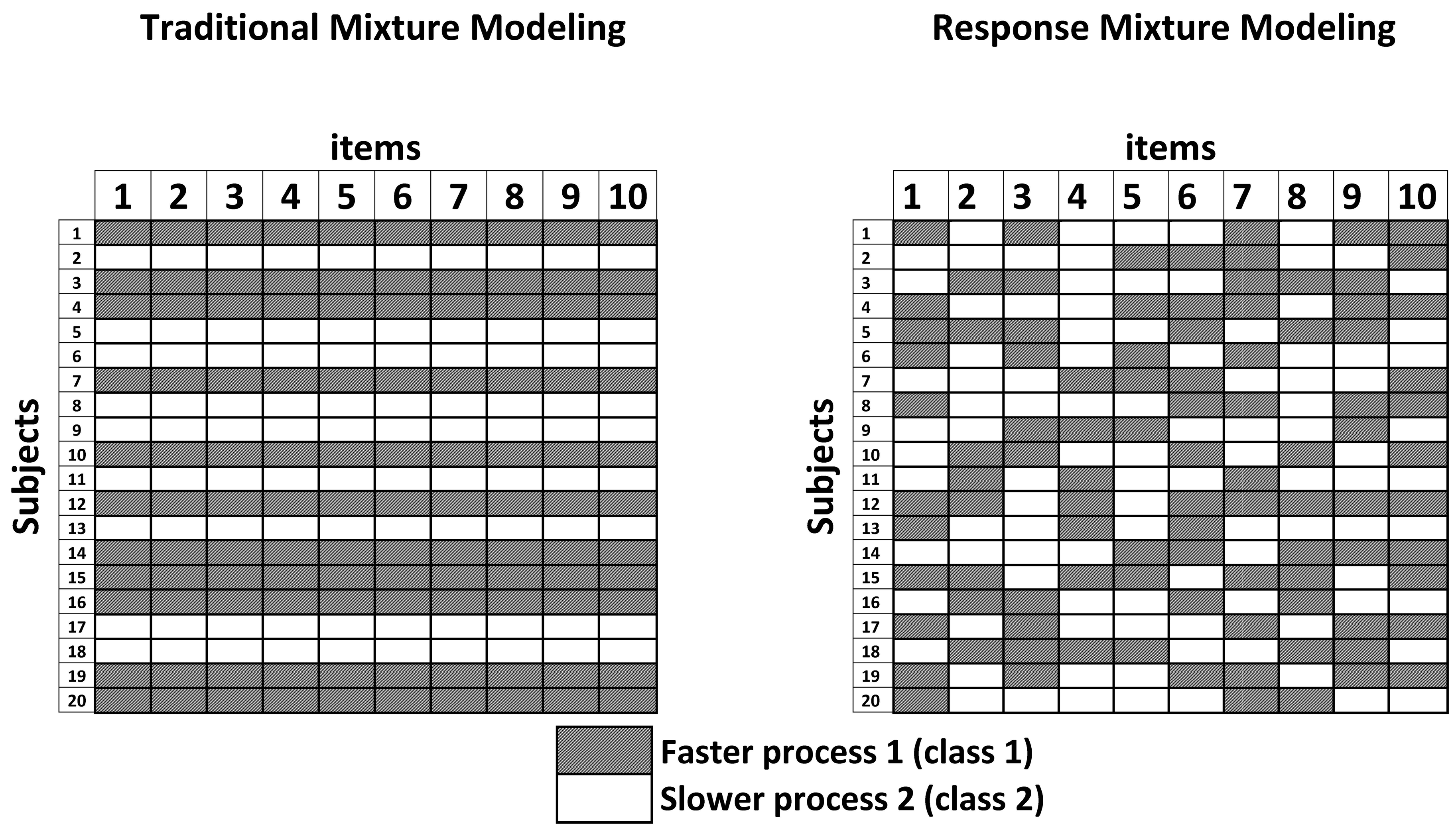
2.2. An Extension to Model Intraindividual Differences

Here, we retain the idea of separate measurement models for the responses and log-response times. That is, for the response times we use Equation (2). However, for the responses, we follow Partchev and De Boeck [25] and we use a separate two-parameter measurement model for the faster responses (“faster measurement model”) and a separate two-parameter measurement model for the slower responses (“slower measurement model”). We avoid the necessity of median splitting the response times by formulating the overall model for the responses as a mixture of the faster and slower measurement models, that is:

$$P(X_{pi}=1{|\mathsf{\theta }}_p^{(s)},{\mathsf{\theta }}_p^{(f)})={\mathsf{\pi }}_{pi}P(X_{pi}=1{|\mathsf{\theta }}_p^{(s)})+(1-{\mathsf{\pi }}_{pi})P(X_{pi}=1{|\mathsf{\theta }}_p^{(f)})$$

(4)

where π_pi is the mixing proportion which denotes the probability that subject p answers item i using the slower latent variable, θ_p^(s), as opposed to faster latent variable θ_p^(f). The faster and slower measurement models are then given by, respectively:

$$logit[P(X_{pi}=1{|\mathsf{\theta }}_p^{(s)})]={\mathsf{\alpha }}_i^{(s)}{\mathsf{\theta }}_p^{(s)}-{\mathsf{\beta }}_i^{(s)}$$

(5)

and

$$logit[P(X_{pi}=1{|\mathsf{\theta }}_p^{(f)})]={\mathsf{\alpha }}_i^{(f)}{\mathsf{\theta }}_p^{(f)}-{\mathsf{\beta }}_i^{(f)}$$

(6)

where

(θ_p^(f), θ_p^(s), τ_p) ~ dmvnorm(µ, Σ)

(7)

with

$$\mathsf{\mu }=[\begin{array}{ccc}{\mathsf{\mu }}_{\mathsf{\tau }}& {\mathsf{\mu }}_{\mathsf{\theta }}^{(s)}& {\mathsf{\mu }}_{\mathsf{\theta }}^{(f)}\end{array}];\mathbf{\Sigma }=\left[\begin{array}{ccc}{\mathsf{\sigma }}_{\mathsf{\tau }}^2& & \\ {\mathsf{\sigma }}_{\mathsf{\tau }\mathsf{\theta }}^{(s)}& {\mathsf{\sigma }}_{\mathsf{\theta }}^{2(s)}& \\ {\mathsf{\sigma }}_{\mathsf{\tau }\mathsf{\theta }}^{(f)}& {\mathsf{\sigma }}_{\mathsf{\theta }}^{(s)(f)}& {\mathsf{\sigma }}_{\mathsf{\theta }}^{2(f)}\end{array}\right]$$

(8)

That is, the latent variables are multivariate normal and are allowed to covary.

To specify the faster responses as indicators in the faster measurement model and the slower responses as indicators in the slower measurement model, the mixing proportion π_pi is made a function of the residual response time, ε_pi. That is:

$$logit({\mathsf{\pi }}_{pi})={\mathsf{\zeta }}_{1i}({\mathsf{\epsilon }}_{pi}-{\mathsf{\zeta }}_{0i})$$

(9)

where parameter ${\mathsf{\zeta }}_{1i}$ is the faster-slower slope parameter which models the degree to which item i can distinguish between the faster and slower classes. That is, for larger ζ_1i, the item contains more information about the different measurement models for faster and slower responses. This parameter is constrained to be non-negative to ensure that the parameters in the slower measurement model (i.e., α_i^(s) and β_i^(s)) correspond to the measurement properties of the slower responses (i.e., larger ε_pi). The parameter ζ_0i is a threshold parameter, which indicates how many responses are classified as slower for item i. The larger ζ_0i is, the less responses are classified as “slower”. That is, due to this parameterization, ζ_0i can be interpreted as the “difficulty” to respond slowly. From the parameter estimates for ζ_1i, ζ_0i, and σ_εi², the class size of the slower class, π_i^(s), can be calculated for each item.1 Note that the item median split procedure used by Partchev and De Boeck [25] assumes that π_i^(s) = 0.5 which corresponds to ζ_0i = 0.

In Equation (9), note that the residual response time, ε_pi, does not include the main effect of the subjects and the main effect of the items on the log-response times. Therefore, a given response is more likely to be classified into the faster/slower measurement model if the response is faster/slower than expected for that subject on that item. For instance, a response of 2 s to a given item can be classified as “faster” for one subject but as “slower” for another subject depending on the subjects’ overall level of speed, τ_p. Similarly, a response of 2 s for a given subject can be classified as “faster” for one item but as “slower” for another item depending on the intensity of the items, λ_i. This is the key difference with interindividual mixture modeling which classifies subjects and not the separate responses into the mixture components. As the model above is a generalization of the response mixture model by Molenaar and De Boeck [29] as we discuss below, we also refer to the model above as response mixture model. Note that the model assumes that the faster and slower classes hold within all subjects in the population. However, the posterior class probability for each subject-item combination (π_pi) may reveal that a given subject hardly uses one of the classes, suggesting that there is only a single process for this subject.

To identify the full model above, some constraints are necessary. To identify the scales and location of the latent variables, σ_τ² = σ²_θ^(s) = σ²_θ^(f) = 1 and μ = {0,0,0} respectively. If restricted versions of the model are considered, for instance a model with α_i^(s) = α_i^(f), some of these constraints can be dropped, that is σ_θ^(s) or σ_θ^(f) can be freed allowing for a scalar effect of the faster/slower response class on the discrimination parameters. Similarly, in a model with β_i^(s) = β_i^(f), the mean of the faster or slower latent variable can be freed, μ^(s) or μ^(f), allowing for a scalar effect on the difficulty parameters.

Special Cases

As discussed, the intraindividual differences model above is a generalization of the response mixture model by Molenaar and De Boeck [29]. That is, if in the model above, one uses the same latent variable in the faster and slower measurement models (i.e., cor(θ^(s), θ^(f)) = 1), and if ζ_0i and ζ_1i are fixed to be equal across items (i.e., ζ_0i = ζ₀, and ζ_1i = ζ₁), the model is equivalent to the model by Molenaar and De Boeck.

The traditional model in Equations (1)–(3) can be obtained from the full model by specifying θ^(s) and θ^(f) to be psychometrically fully equivalent. Equivalence of θ^(s) and θ^(f) implies that α_i^(s) = α_i^(f), β_i^(s) = β_i^(f), cor(θ^(s), θ^(f)) = 1, σ²_θ^(s) = σ²_θ^(f), and ζ_1i = 0. Given these restrictions, π_pi will cancel out Equation (4) because it will hold that $P(X_{pi}=1{|\mathsf{\theta }}_p^{(s)})$ = $P(X_{pi}=1{|\mathsf{\theta }}_p^{(f)})$, as a result, parameter ζ₀ will not be in the model anymore.

2.3. Conditional Dependence

As discussed above, in the traditional interindividual differences model outlined by Equations (1)–(3), it is assumed that conditional on the latent speed and the latent ability variable, τ_p and θ_p, the responses and response times of item i are independent. In the intraindividual extension of this model outlined by Equations (4)–(9), conditional dependence is explicitly modeled: If ζ_1i in Equation (9) deviates from 0, the measurement properties of the responses depend on the length of the response times. That is, there are intraindividual differences in the measurement model that applies to the responses, reflecting the use of different response processes.

Any phenomenon that leads to fluctuations in ability and speed throughout the test administration will result in violations of conditional independence between responses and response times [43]. Therefore, if subjects make more (or less) errors and respond faster (or slower) throughout the test irrespective of the difficulty and the time intensity of the items, conditional independence will be violated. This may for instance happen due to practice, decreased motivation, or increased fatigue throughout the test administration. Such a trend will be captured by the faster and slower classes in the present approach. This will be evident from the results. That is, in the case of learning, the faster response class will be larger (larger ζ_0i) and less difficult (smaller β_1i) for later items. In the case of a decreased motivation (faster responses with more errors for later items), the faster response class will be larger but the items will be more difficult in this class. In the discussion we return to this point.

2.4. Estimation

We implemented a Bayesian Markov Chain Monte Carlo procedure (MCMC; see, e.g., [44]) within the OpenBUGS software package [45]. To this end we specified N(0,10) prior distributions for the parameters β_i^(s), β_i^(f), ϕ_i, and λ_i. In addition, for the parameters α_i^(s), and α_i^(f) we specified N(0,10) prior distributions that are truncated below 0.01 to ensure that the parameter values are strictly positive. For ζ_1i, we truncated the N(0,10) prior below 0. We specified a N(0,10) on log(σ_ε²). We scaled the latent variable by fixing their variances to equal 1, therefore, Σ is a 3 × 3 correlation matrix, which we decompose as follows:

Σ = ΓΓ^T + diag(1₃ − Γ²)

(10)

where Γ is a 3 × 1 column vector with parameters γ_k for k = 1, 2, 3 and 1₃ is a 3 × 1 column vector of 1 s. For each element of Γ we specified a uniform prior from −1 to 1. Finally, in Equation (9), ε_pi does not need to be estimated from the data, as it can be calculated by:

$${\mathsf{\epsilon }}_{pi}=T_{pi}^{*}-{\mathsf{\phi }}_i{\mathsf{\tau }}_p-{\mathsf{\gamma }}_i$$

(11)

that is, the residual response time is the log-response time corrected for the main effect of the subjects and the main effect of the items. See the website of the first author for the OpenBUGS script.

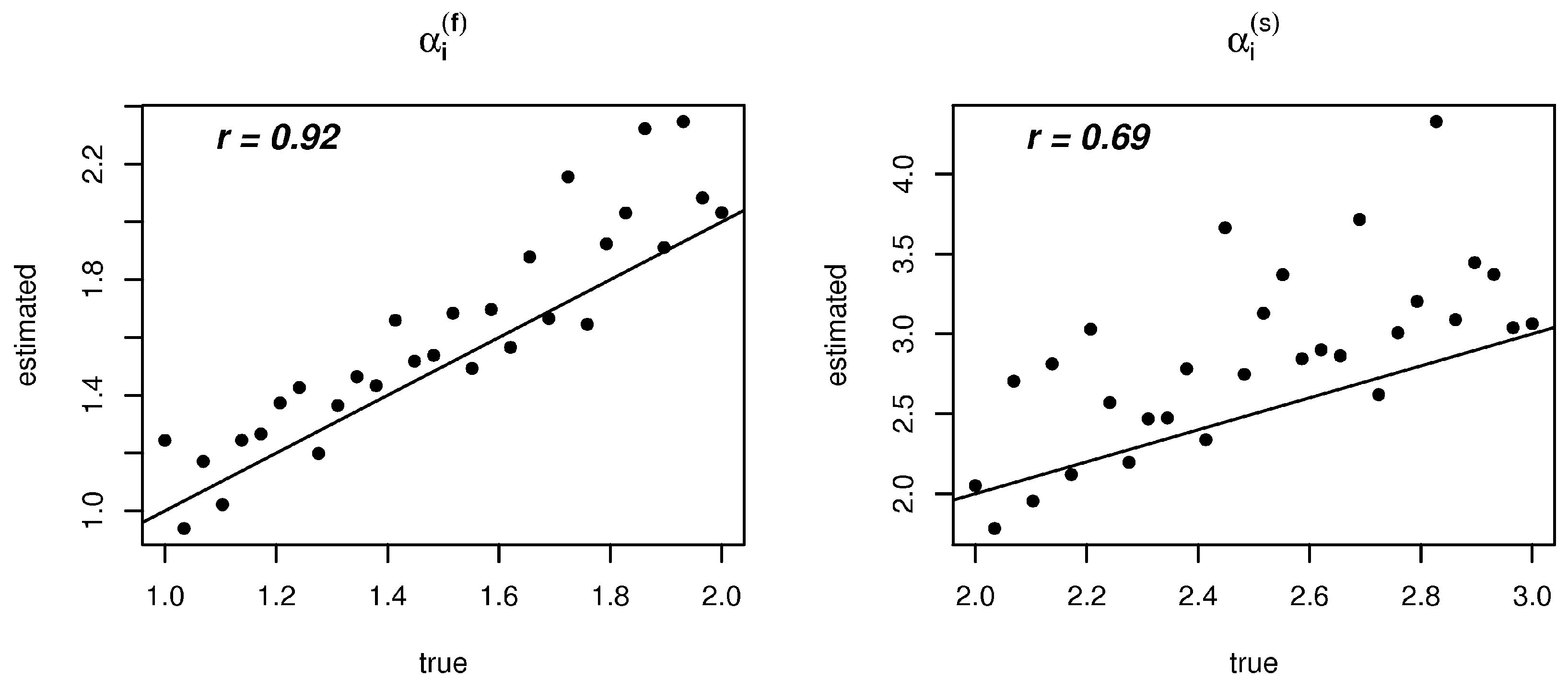
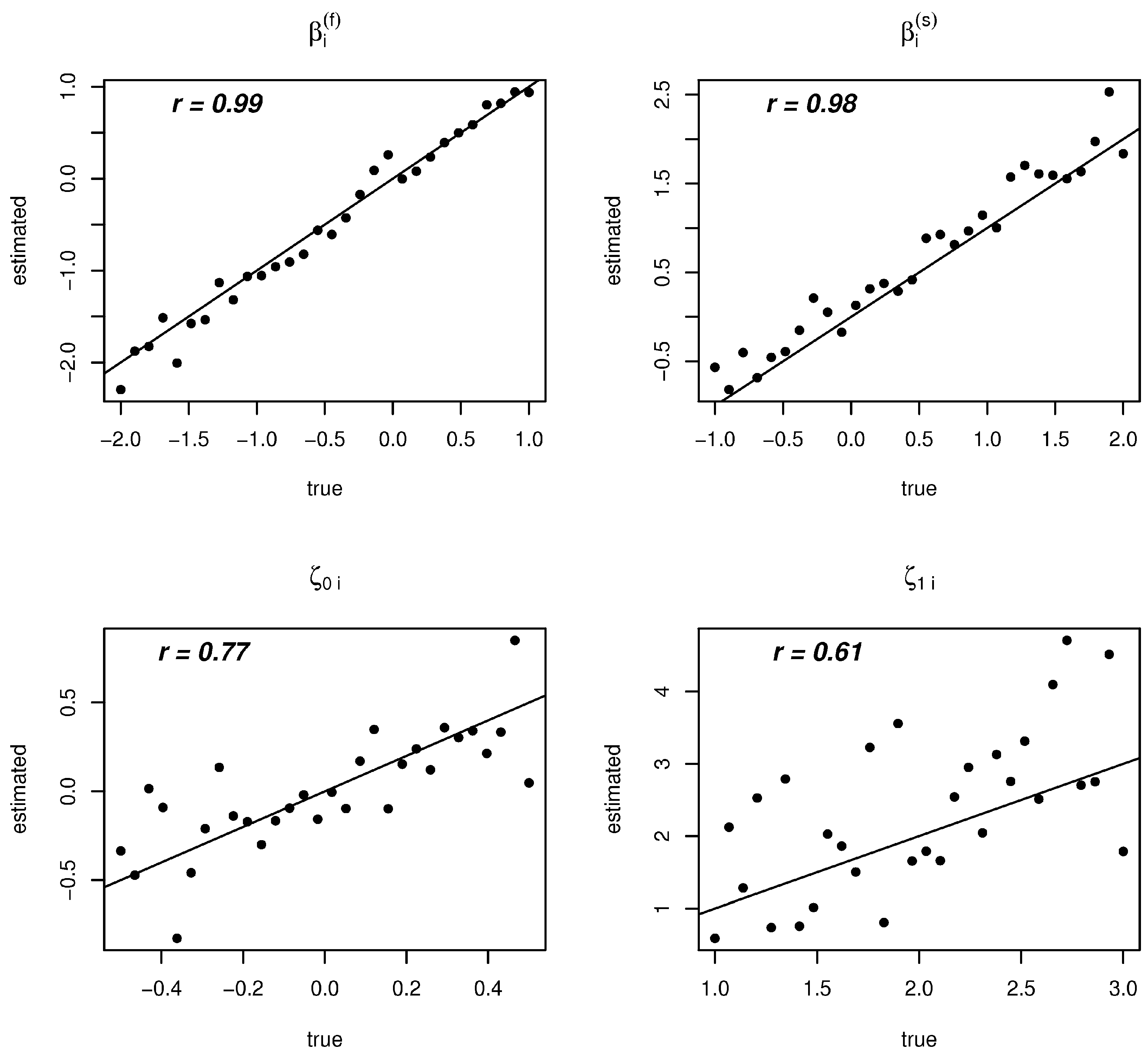
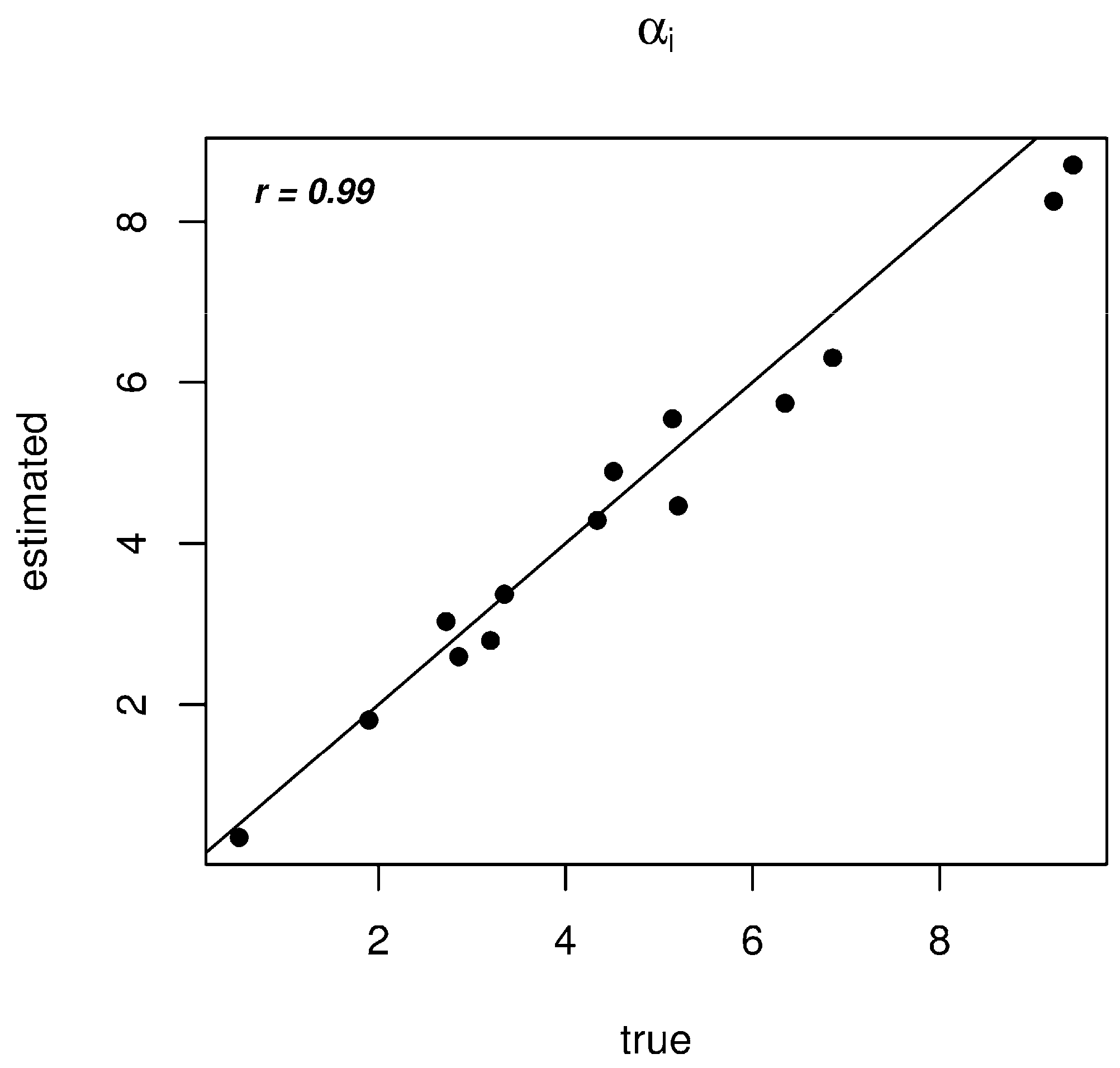
3. Simulated Data Application

3.1. Data Generation

To show the viability of the present approach, we applied the response mixture model to a simulated data set. Data were simulated using 2000 subjects and 30 items. The following true parameter values were used: First, for the discrimination parameters we created of a vector of increasing and equally spaced values that were subsequently assigned randomly to the items 1 to 30. For α_i^(f) we used values between 1 and 2 and for α_i^(s) we used values between 2 and 3 to reflect that slower responses discriminate better than faster responses (i.e., according to the “worst performance rule” [28]). For the difficulty parameters we used increasing, equally spaced values between ‒2 and 1 for β_i^(f) and between −1 and 2 for β_i^(s) to reflect that faster responses are associated with less errors as compared to slower responses [25]. Next, for ζ_0i we used increasing and equally spaced values between −0.5 and 0.5. Note that the items are thus ordered on both their difficulty (β_i^(s) and β_i^(f)) and their threshold parameter (ζ_0i) reflecting that the harder the item, the more likely subjects are to resort to slower processes. This relation between item difficulty and the slower process has been chosen based on the real data application below. For the true values of the slope parameters, ζ_1i, we created of a vector of increasing and equally spaced values between 1 and 3 that were subsequently assigned randomly to the items 1 to 30. In addition, the correlations in Σ were fixed to cor(θ^(s), θ^(f)) = 0.8, cor(τ, θ^(s)) = −0.6, and cor(τ, θ^(f)) = −0.7. Note that although these correlations are large, they are not exceptional as for the Block Design application below, we found even larger correlations. Finally, the other parameters were fixed to: ϕ_i = 2, σ_εi² = 3, λ_i = 2 for all i.

3.2. Results

Using our OpenBUGS implementation of the model, we drew 150,000 samples from the posterior parameter distribution of which we discarded the first 75,000 samples as burn-in. Preliminary data simulations showed that this is sufficient to ensure convergence of the chain to its stationary distribution. In Figure 2, trace plots are depicted for the parameters α_i^(f), α_i^(s), ζ_0i, and ζ_1i for item 1, trace plots for the other parameters were similar. As can be seen, after the burn-in samples (solid grey line), the samples scatter randomly around a stable average.

In Figure 3, the true parameter values are plotted against the estimated values. As can be seen, for β_i^(s), β_i^(f), α_i^(f), and ζ_0i parameter recovery is good. For the α_i^(s) and ζ_1i parameters, estimates are characterized by larger variability as compared to the other parameters. In addition, they tend to be slightly biased. However, given the large variability in the parameter estimates the bias does not seem to be severe. We investigate this possible bias in more depth in the application section where we simulate data given the results of the block design data. With respect to the variability in the parameter estimates, it can be concluded that the power to reject the restriction α_i^(s) = α_i^(f) will generally be small. In practice it seems, thus, advisable to consider restricting α_i^(s) = α_i^(f). In addition, ζ_1i could be constrained to be equal across items to decrease parameter variability in this parameter. We will consider these possibilities in the real data application next.

4. Application to the Wechsler Intelligence Scale for Children-Fourth Edition (WISC-IV) Block Design Test

4.1. Data

Here we present an analysis of the Hungarian standardization data of the Block Design subtest from the Wechsler Intelligence Scale for Children-Fourth Edition (WISC-IV [30,31]). This test involves arranging colored blocks as fast as possible into a displayed pattern. There are 14 items that are scored 1 (correct) and 0 (false). Response times are recorded starting at the moment that the subject was presented with the item until the moment that the subject indicated that he or she was finished, gave up, or the time was up. The number of subjects equals 978 with an age range between 6 and 15. Preliminary analysis indicated that measurement invariance of the response and response time measurement model in Equations (1)–(3) is tenable for older and younger subjects. The older subjects are overall more accurate and faster with more variance in their responses and response times (as reflected in a significant difference in the mean and variance of both θ and τ; results are available upon request). These differences between the younger and older subjects may reflect differences in response processes across ages. For instance, as shown by Rozencwajg and Corroyer [46], children of different ages use the same processes (global and analytic), but older children use the analytic process more often than the global processes. Therefore, we think that for our modeling approach, the differences between young and old as reported above are not necessarily a problem as these differences will be captured in the response class membership of the subjects (i.e., the responses of the older subjects—which are overall faster and more accurate—will be classified more often in a fast and accurate response class and less often in a slow and inaccurate response class).

Proportions correct for the 14 items are 0.999, 0.991, 0.980, 0.942, 0.906, 0.876, 0.835, 0.707, 0.705, 0.625, 0.489, 0.505, 0.377, and 0.210, respectively. The response times are between 1 and 360 s such that the log-response times are between 0 and 6, see Figure 4 for a box plot of the log-response time distributions.

4.2. Results

4.2.1. Conditional Independence

As violations of conditional independence indicate intraindividual differences in the response measurement properties across response times, we started by testing for conditional independence between the responses and response times of the items. Specifically, we fit the traditional model in Equations (1)–(3) to the data using weighted least squares estimation in Mplus [47] with and without residual correlations between the responses and response times of the items. Note that the model with residual correlations between the responses and response times is identical to the model proposed by the authors of [36]. For other more Bayesian oriented approaches see References [48,49].

For each item we consulted (1) the univariate modification index of the correlation between the responses and the response times in the traditional model (i.e., the model without residual correlations); and (2) the size of the residual correlation between the responses and response times in the model with residual correlations. The modification indices are related to the Lagrange multiplier test [50] proposed by the authors of [43] to test the assumption of conditional independence of responses and response times. Modification indices are chi-square distributed with 1 degree of freedom and indicate the impact of a parameter constraint on the log-likelihood of the model. Note that the modification indices are estimated under the assumption that conditional independence holds for all other items. See

Table 1. Modification indices (Mod.) and residual correlations (Cor.) between the responses and response times of the items.

Item	Mod.	Cor.
1	28.59	0.35
2	1.41	−0.16
3	7.87	−0.12
4	6.06	−0.07
5	14.24	−0.11
6	13.14	−0.15
7	8.41	−0.13
8	5.59	−0.11
9	12.44	−0.14
10	7.44	−0.11
11	14.37	−0.13
12	14.99	−0.13
13	24.46	−0.16
14	70.64	−0.16

Note: Mod. are obtained in a model without residual correlations between responses and response times, while Cor. are obtained in a model with residual correlations.

for both the modification indices and the residual correlations. As can be seen, conditional independence is clearly violated for most of the items, although effect size is small. This finding is in line with [43] who found this type of conditional independence being violated in most of the items in a large-scale computerized test. Interestingly, the residual correlations are negative for all items but item 1, indicating that slower responses (higher ε_pi) are associated with a smaller probability of a correct response. This is not due to the brighter subjects being faster, as the residual correlation is separate from the main ability and speed effects (as these are captured by the respective latent variables).

4.2.2. Response Mixture Models

To investigate how faster responses differ in their measurement properties as compared to slower responses, we resorted to the response mixture models outlined in this paper. We fit different models to the data. First, the traditional model from Equations (1)–(3) was fit as a baseline model (Model #0; i.e., a model without mixtures, as discussed above). For this model, we run 10,000 iterations with 5000 as burn-in as this was already sufficient for convergence.

Table 2. Model #0: Means and standard deviations (sd) for the samples from the posterior distribution of the parameters in the measurement model for the responses.

i	αi		βi
	mean	sd	mean	sd
1	0.56	0.43	−6.91	0.91
2	1.74	0.39	−6.13	0.68
3	2.79	0.48	−6.84	0.83
4	2.76	0.33	−5.16	0.47
5	3.05	0.32	−4.59	0.39
6	3.42	0.37	−4.37	0.41
7	3.54	0.35	−3.76	0.35
8	4.56	0.43	−2.55	0.28
9	3.99	0.36	−2.09	0.24
10	4.58	0.41	−1.16	0.22
11	5.32	0.57	0.90	0.25
12	5.62	0.62	0.86	0.26
13	4.42	0.48	2.32	0.30
14	1.82	0.20	2.34	0.19

depicts the discrimination parameters (α_i) and the difficulty parameters (β_i) for the baseline model. In this model, no distinction is made between a faster and a slower measurement model. That is, this model is misspecified with respect to conditional dependence. As can be seen, the items increase in their difficulty and the discrimination parameters differ notably between items. In addition, the parameters of item 1 and 2 are associated with relatively large uncertainty (reflected by the large standard deviation of the parameters). This is due to the large proportion correct for these items (i.e., only 1 and 8 subjects failed on these items, respectively).

Next, a series of response mixture models was fit to the data. For the response mixture models, we run two chains of 500,000 iterations each. We omitted the first 250,000 as burn-in. To check whether the MCMC sampling scheme converged to its stationary distribution we considered trace plots of the parameters and the Gelman and Rubin statistic on the equality of the variance across the two chains [51]. First, from the trace plots all chains seemed to vary randomly around a stable average. Second, the Gelman and Rubin statistic for all parameters were close to 1.00.

Table 3. DIC, mAIC, and mBIC model fit statistics for the models considered in the application.

Model	Restriction(s)	DIC	mAIC	mBIC
1	–	25,850	30,464	33,494
2	αi(s) = αi(f)	25,690	30,389	33,407
3	αi(s) = αi(f); βi(s) = βi(f)	25,900	30,474	33,479
4	αi(s) = αi(f); ζ1i = ζ1	25,570	30,232	33,236
5	αi(s) = αi(f); ζ1i = ζ1; ζ0i = ζ0	25,940	30,339	33,329

Note: The best values for the fit indices are in boldface.

depicts the Deviance Information Criterion (DIC [52]), and a modified version of the Akaike’s Information Criterion [53] and the Bayesian Information Criterion [54], referred to as mAIC and mBIC, respectively. The mAIC and mBIC have been proposed by Molenaar and De Boeck [29] for model comparison in response mixture models.2 In addition,

Table 4. Parameters for the latent variables in the models considered.

Model	Restriction(s)	Correlations			σθ(s)	µθ(s)
		θ(s), θ(f)	τ, θ(s)	τ, θ(f)
0	–	–	−0.90 1	–	–	–
1	–	0.95	−0.90	−0.86	1 *	0 *
2	αi(s) = αi(f)	0.95	−0.90	−0.86	1.20 (0.16)	0 *
3	αi(s) = αi(f); βi(s) = βi(f)	0.96	−0.89	−0.87	1.05 (0.06)	−0.97 (0.06)
4	αi(s) = αi(f); ζ1i = ζ1	0.93	−0.91	−0.86	1.18 (0.14)	0 *
5	αi(s) = αi(f); ζ1i = ζ1; ζ0i = ζ0	0.96	−0.89	−0.87	0.98 (0.09)	0 *

Note: Posterior standard deviations are in brackets. Model #0 is the baseline model as defined by Equations (1)–(3); * these parameters are fixed for identification purposes. Note that for all models μ_θ^(f) = 0 and σ²_θ^(f) = 1; ¹ this is the correlation between τ_p and θ_p as there is not distinction between a faster and slower latent variable in this model.

contains the correlations between the latent variables in the different models together with σ_θ^(s) and μ_θ^(s). As can be seen from the tables, a full model was considered with all parameters free (Model #1). In this model, the faster and slower latent variables are highly correlated as is also found by Partchev and De Boeck [25]. We do not compare the full model to the baseline model (Model #0) in terms of the DIC, mAIC and mBIC fit indices as the models contain a different number of random effects (two in the baseline model and three in the full model), which distorts model comparison (see, e.g., [55,56]). However, given that we found that conditional independence was violated for most of the items (see above), it is suggested that the full model should be preferred over the baseline model.

Next, we considered Model #2 with equal discrimination parameters across the faster and slower measurement models (α_i^(s) = α_i^(f)) but with the standard deviation of the slower latent variable, σ_θ^(s), free to allow for a uniform effect on the discrimination parameters. This model fit the data better in terms of the DIC, mAIC, and mBIC as compared to the full model (Model #1). We therefore proceeded by retaining the restriction on the discrimination parameters and additionally constraining the difficulty parameters for the faster and slower responses to be equal (β_i^(f) = β_i^(s)). We freed the mean of the slower latent variable variable, μ^(s), to allow for a scalar effect on the difficulty parameters. This resulted in Model #3. The model fit the data worse as compared to Model #2 in terms of the DIC, mAIC, and mBIC. We therefore concluded that the difficulty parameters differ across faster and slower responses. In Model #4, we allowed the difficulty parameters to differ again between the faster and slower responses; however, we constrained the slope parameters, ζ_1i, to be equal across items (ζ_1i = ζ₁). This restriction resulted in an improved DIC, mAIC, and mBIC as compared to Model #3. Additionally constraining ζ_0i to be equal across items (ζ_0i = ζ₀; Model #5) resulted in a deterioration in model fit.

As Model #4 is the best fitting model, we conclude that the slope parameters ζ_1i are equal across items [ζ_1i = ζ₁], that the discrimination parameters are equal for the faster and slower classes [α_i^(s) = α_i^(f)], but that the difficulty parameters are different for the faster and slower classes [β_i^(s) ≠ β_i^(f)]. In addition, the faster and slower response class sizes are unequal across items [ζ_0i ≠ ζ₀]. In Model #4, the estimate for ζ₁ equaled 10.72 (sd: 1.296; 95% Highest Posterior Density region, HPD: 8.46; 13.52), which is large because its scale depends on the scale of ε_pi. That is, for all items, σ_εi² equaled between 0.20 and 0.45.

As Model #3 is rejected in favor of Model #4, it can be concluded that the differences in the faster and slower difficulty parameters do not only reflect an overall effect (i.e., a difference in μ_θ^(s) and μ_θ^(f)) but also additional item specific effects. For the faster and slower discrimination parameters that are shown to be equal for the faster and slower classes, there may still be an overall effect in Model #4 as σ_θ^(s) is estimated freely. That is, in Table 4, it can be seen that the estimate for σ_θ^(s) in Model #4 equaled 1.18. It is interesting to see whether this parameter deviates from 1 as this will indicate that the slower responses discriminate overall better (as σ_θ^(s) > 1 see Table 4) than the faster responses (as σ_θ^(f) = 1 for identification reasons). However, the 95% HPD region for σ_θ^(s) runs from 0.93 to 1.48, thus, as this interval contains 1, there is no clear evidence against the assumption that faster and slower responses discriminate equally well in the WISC data.

For the estimates of α_i, β_i^(f), β_i^(s), and ζ_0i in Model #4, see

Table 5. Model #4: Posterior parameter means and standard deviations of the parameters in the measurement model for faster and slower responses and the mixing threshold parameters together with the size of the slower response class (π_i^(s)).

i	αi		βi(f)		βi(s)		ζ0i		πi(s)
	mean	sd	mean	sd	mean	sd	mean	sd
1	0.51	0.40	−3.01	4.21	−4.36	3.83	−0.39	3.99	0.65
2	1.90	0.47	−6.45	1.56	−1.58	2.81	2.30	1.93	0.01
3	2.72	0.54	−7.62	1.02	−2.99	1.86	1.33	0.26	0.10
4	2.86	0.45	−6.55	0.80	−3.30	0.69	0.54	0.10	0.30
5	3.35	0.44	−5.85	0.61	−2.19	0.67	0.63	0.09	0.27
6	4.34	0.55	−6.22	0.70	−1.37	0.94	1.01	0.08	0.16
7	4.51	0.56	−5.58	0.63	−1.97	0.74	0.74	0.10	0.23
8	5.21	0.59	−3.84	0.47	−0.95	0.59	0.52	0.10	0.30
9	5.14	0.60	−3.81	0.47	−0.42	0.55	0.46	0.10	0.33
10	6.35	0.82	−2.75	0.47	0.82	0.64	0.42	0.09	0.34
11	9.42	1.35	−0.95	0.50	5.88	1.31	0.32	0.06	0.38
12	9.22	1.23	−1.45	0.51	6.18	1.22	0.28	0.05	0.39
13	6.86	0.97	0.49	0.41	7.81	1.30	0.13	0.05	0.45
14	3.20	0.47	1.36	0.30	7.68	1.27	0.11	0.04	0.46

. From the 95% HPD regions it appeared that only ζ_0i departures from 0 for all items, except item 1 and 2. Indicating that the faster and slower response class sizes are unequal (i.e., they depart from 0.5). In addition, Table 5, contains the size of the slower response class (π_i^(s)) on each item can be determined from the estimates of ζ_0i, ζ₁, and σ_εi². As can be seen, the slower response class is used more often for the items at the end of the test. As the items are administered in order of difficulty (as can also be seen in Table 2, the difficulty increases for increasing item number), this result suggests that for more difficult items, respondents resort more to slower response processes. With respect to the β_i^(s) and β_i^(f) parameters estimates, it can be seen that they differ substantially. In Figure 5 this difference is graphically displayed. For all items the difficulty parameters are larger for the slower responses, except for item 1 (which explains the negative residual correlations in Table 1).

To investigate whether the results above are stable and do not depend too much on the exact choice concerning the parameter restrictions, we also present the results for the model with equal mixing parameters across items (i.e., ζ_0i = ζ₀; ζ_1i = ζ₁). In this model, ζ₀ was estimated to be 0.32 (95% HPD: 0.27; 0.37) and ζ₁ was estimated to be 10.00 (95% HPD 7.61; 13.08). From the results (not displayed) it appeared that the differences between the faster and slower difficulty parameters are somewhat smaller, however, the general effect from Figure 5 is still visible.

Simulation. As parameters α_i^(s) and ζ_1i tend to be slightly biased in the simulation study, we investigated whether this is also the case given α_i = α_i^(s) = α_i^(f) and ζ_1i = ζ₁ as found above. That is, we simulated data using the exact setup as in the application above. We used the final model, Model #4, and fit Model #4 to these simulated data to see whether the α_i, σ_θ^(s), and ζ₁ parameters are adequately recovered. See Figure 6 for a plot of the true values of α_i against the estimated values. As can be seen, the true values are adequately recovery. In addition, the estimate for σ_θ^(s) equaled 1.42 (95% HPD: 1.09; 1.78) where the true value is 1.18 (see Table 4), and the estimate of ζ₁ equaled 9.22 (95% HPD: 7.61; 11.14) where the true value is 10.72 (see above). Thus, we think that the true values are adequately recovered given the parameter variability.

5. Discussion

This paper was motivated by the finding of Partchev and De Boeck [25] that for a Matrix Reasoning and a Verbal Analogy intelligence subtest, faster responses load on a different latent variable with different item difficulty parameters than slower responses. In this paper, we followed up on this finding by (1) replicating the Partchev and De Boeck findings in the Block Design subtest of the WISC; (2) by additionally testing whether item discrimination parameters differ across faster and slower responses; and (3) by testing whether the faster and slower response class sizes are unequal and whether they differ across items.

The results show that slower responses discriminate about equally well as compared to the faster responses. This finding is in contrast with the “worst performance rule” [28], which predicts that slower responses contain more information about individual differences in ability than faster responses. This contrasting result might be due to a lack of power to detect a difference. That is, in the simulation study it was shown that the slower discrimination parameters are associated with relatively large uncertainties. Although, in the application, we constrained the slower and faster discrimination parameters to be equal, which would be expected to increase the power to detect an overall effect, it is still possible that the power was too small to detect a difference. An in-depth study of the power to detect unequal discrimination parameters across faster and slower responses given realistic effect sizes seems valuable therefore.

On the other hand, the failure to find differences in discrimination between faster and slower responses may suggest that the worst performance rule, which is typically established using experimental task with very fast responses (500–1000 ms), does not hold for cognitive ability tasks with responses that are substantially larger. For instance, the authors of [57] tested the worst performance rule by correlating measures of fluid intelligence to the response times on a psychomotor vigilance task. It was found that the higher quantiles of the response times correlated stronger with fluid intelligence. However, response times on the psychomotor vigilance task were on average 274 ms for the first quantile and 484 ms for the fifth quantile while in the present study, response times to the block design task are between 1 and 360 s.

A second finding in the application is that slower responses are associated with less accuracy than faster responses. This finding is in line with both [18,25]. It suggests that some responses take longer because these responses are based on processes that are more error prone and inefficient as compared to the faster responses. A final finding was that the faster and slower response class sizes are unequal and differ across items with the slower response class being larger for the more difficult items. Overall, the most important finding of the present study and the Partchev and De Boeck study [24] is that faster responses differ in their measurement properties from the slower responses. This result indicates that a different intraindividual process underlies the responses to the different items. In establishing this, both in the present study and in the Partchev and De Boeck study it was assumed that the response times can be separated into the binary categories of faster and slower responses. This binary distinction can reflect a true dichotomy underlying the response times, as is the case in for instance a dual processing framework [17,18]. For the present application to the WISC block design subtest, the faster process might be a more analytic process and the slower process might be a more global process (e.g., [24]). The exact substantive interpretation of the faster and slower response class however need to be established using additional covariates. For instance, covariates like test taking behavior (“trial and error” or “pattern memorization”), brain-imaging data, or eye tracking information can be used to establish the nature of the two classes.

However, our results do not mean that there needs to be a true dichotomy underlying the response processes of the block design subtest. That is, in our application we have used a dichotomy, but in reality there may be multiple processes. For instance, Rozencwajg and Corroyer [46] argued for a third, syntactic process to underlie the block design. This does not invalidate the present results as in the case of multiple processes (e.g., A, B, C, D, E, and F), the faster and slower latent variables will capture the variation in the item responses by the faster processes (e.g., A, B, and C) on the one hand and the variation by the slower processes on the other hand (e.g., D, E, and F). Adopting a modeling approach with more than two classes is possible in principle, but identification and estimation of such a model is highly challenging. Other possibilities might be that a continuous mode of processing, or a sequential use of processes (i.e., subjects use the slow process whenever the fast process was unsuccessful) exist in reality. Then again, our approach can still capture the most important patterns in the data (i.e., differences between the faster and slower responses).

Another result that needs discussion is the almost perfect correlation that was found between the fast and slow latent ability variables. This result indicates that there is only one dimension of interindividual differences underlying the block design test. As the item difficulties associated with the latent abilities differed across the faster and slower classes, a dimension of intraindividual differences can be distinguished as well. That is, the slower responses have different measurement properties as compared to the faster responses suggesting a different response processes, but the underlying dimension of interindividual differences is the same. This result is similar to what is found by DiTrapani, Jeon, De Boeck, and Partchev [27].

As we showed that intelligence subtests may be potentially heterogenous with respect to the intraindividual processes that are measured, the results imply that for a given test administration one should decide whether this source of intraindividual variation is considered desirable or a confound. That is, does the intraindividual variation contribute to the validity of the test (e.g., [13]) or does it provide a confound that should be eliminated (e.g., [58]). In the case of arithmetic tests for instance, the heterogeneity in intraindividual processes may be considered desirable as the test taps into both memory retrieval and problem solving, which are both aspects of arithmetic [19].

In other settings, differences in response times might be seen as a confound. For instance, undesirable strategies such as faking on some of the items of a test [59], the use of item preknowledge [60], learning and practice effects [2], post error slowing [61], and fatigue and motivation issues [62], will all result in intraindividual variation that harms the validity of an intelligence test. In addition, the authors of [58] discusses how different speed-accuracy compromises can be seen as a confound. That is, subjects differ in the amount of time they use to solve a given item. Therefore, an incorrect response may indicate either that the subject didn’t use enough time or it may reflect the inability to solve that item. As a solution, [63] proposed the response signal paradigm. In this paradigm a subject can only respond to a test item at a given moment after the item is presented (e.g., after 20 s). Therefore, all response times will be equal for all subjects, which standardize the speed-accuracy tradeoff within and between subjects. Heterogeneity may therefore be decreased because some (but not all) subjects are not allowed enough time to solve a given item using a more accurate but more time-consuming response process.

References

1. Raven, J.C. Advanced Progressive Matrices; HK Lewis: London, UK, 1962. [Google Scholar]
2. Carpenter, P.A.; Just, M.A.; Shell, P. What one intelligence test measures: A theoretical account of the processing in the Raven Progressive Matrices Test. Psychol. Rev. 1990, 97, 404–431. [Google Scholar] [CrossRef] [PubMed]
3. Galton, F. Hereditary Genius: An Inquiry into its Laws and Consequences; Macmillan: Fontana, CA, USA; London, UK, 1869. [Google Scholar]
4. Galton, F. Inquiries into Human Faculty and its Development; AMS Press: New York, NY, USA, 1883. [Google Scholar]
5. Jensen, A.R. Galton’s legacy to research on intelligence. J. Biosoc. Sci. 2002, 34, 145–172. [Google Scholar] [CrossRef] [PubMed]
6. Jensen, A.R. Clocking the Mind: Mental Chronometry and Individual Differences; Elsevier: Amsterdam, The Netherlands, 2006. [Google Scholar]
7. Van Ravenzwaaij, D.; Brown, S.; Wagenmakers, E.J. An integrated perspective on the relation between response speed and intelligence. Cognition 2011, 119, 381–393. [Google Scholar] [CrossRef] [PubMed]
8. Ratcliff, R.; Schmiedek, F.; McKoon, G. A diffusion model explanation of the worst performance rule for reaction time and IQ. Intelligence 2008, 36, 10–17. [Google Scholar] [CrossRef] [PubMed]
9. Ratcliff, R. A theory of memory retrieval. Psychol. Rev. 1978, 85, 59–108. [Google Scholar] [CrossRef]
10. Wagenmakers, E.-J. Methodological and empirical developments for the Ratcliff diffusion model of response times and accuracy. Eur. J. Cogn. Psychol. 2009, 21, 641–671. [Google Scholar] [CrossRef]
11. Van der Maas, H.L.J.; Molenaar, D.; Maris, G.; Kievit, R.A.; Borsboom, D. Cognitive psychology meets psychometric theory: On the relation between process models for decision making and latent variable models for individual differences. Psychol. Rev. 2011, 118, 339–356. [Google Scholar] [CrossRef] [PubMed]
12. Molenaar, D. The value of response times in item response modeling. Measurement 2015, 13, 177–181. [Google Scholar] [CrossRef]
13. Borsboom, D.; Mellenbergh, G.J.; van Heerden, J. The concept of validity. Psychol. Rev. 2004, 111, 1061–1071. [Google Scholar] [CrossRef] [PubMed]
14. Hamaker, E.L.; Nesselroade, J.R.; Molenaar, P.C. The integrated trait-state model. J. Res. Personal. 2007, 41, 295–315. [Google Scholar] [CrossRef]
15. Molenaar, P.C.M. A manifesto on psychology as idiographic science: Bringing the person back into scientific psychology, this time forever. Measurement 2004, 2, 201–218. [Google Scholar] [CrossRef]
16. Van der Maas, H.L.; Dolan, C.V.; Grasman, R.P.; Wicherts, J.M.; Huizenga, H.M.; Raijmakers, M.E. A dynamical model of general intelligence: The positive manifold of intelligence by mutualism. Psychol. Rev. 2006, 113, 842–861. [Google Scholar] [CrossRef] [PubMed]
17. Shiffrin, R.M.; Schneider, W. Controlled and automatic human information processing: II. Perceptual learning, automatic attending and a general theory. Psychol. Rev. 1977, 84, 127–190. [Google Scholar] [CrossRef]
18. Goldhammer, F.; Naumann, J.; Stelter, A.; Tóth, K.; Rölke, H.; Klieme, E. The time on task effect in reading and problem solving is moderated by task difficulty and skill: Insights from a computer-based large-scale assessment. J. Educ. Psychol. 2014, 106, 608–626. [Google Scholar] [CrossRef]
19. Grabner, R.H.; Ansari, D.; Koschutnig, K.; Reishofer, G.; Ebner, F.; Neuper, C. To retrieve or to calculate? Left angular gyrus mediates the retrieval of arithmetic facts during problem solving. Neuropsychologia 2009, 47, 604–608. [Google Scholar] [CrossRef] [PubMed]
20. Ericsson, K.A.; Staszewski, J.J. Skilled memory and expertise: Mechanisms of exceptional performance. In Complex Information Processing: The Impact of Herbert A. Simon; Klahr, D., Kotovsky, K., Eds.; Erlbaum: Hillsdale, MI, USA, 1989. [Google Scholar]
21. Van Harreveld, F.; Wagenmakers, E.J.; van der Maas, H.L. The effects of time pressure on chess skill: An investigation into fast and slow processes underlying expert performance. Psychol. Res. 2007, 71, 591–597. [Google Scholar] [CrossRef] [PubMed]
22. Goldstein, K.; Scheerer, M. Abstract and concrete behavior an experimental study with special tests. Psychol. Monogr. 1941, 53, 1–151. [Google Scholar] [CrossRef]
23. Jones, R.S.; Torgesen, J.K. Analysis of behaviours involved in performance of the block design subtest of the WICS-R. Intelligence 1981, 5, 321–328. [Google Scholar] [CrossRef]
24. Schorr, D.; Bower, G.H.; Kiernan, R. Stimulus variables in the block design task. J. Consult. Clin. Psychol. 1982, 50, 479–487. [Google Scholar] [CrossRef] [PubMed]
25. Partchev, I.; de Boeck, P. Can fast and slow intelligence be differentiated? Intelligence 2012, 40, 23–32. [Google Scholar] [CrossRef]
26. Jeon, M.; de Boeck, P. A generalized item response tree model for psychological assessments. Behav. Res. Methods 2015, in press. [Google Scholar] [CrossRef] [PubMed]
27. DiTrapani, J.; Jeon, M.; De Boeck, P.; Partchev, I. Attempting to differentiate fast and slow intelligence: Using generalized item response trees to examine the role of speed on intelligence tests. Intelligence 2016, 56, 82–92. [Google Scholar] [CrossRef]
28. Larson, G.E.; Alderton, D.L. Reaction time variability and intelligence: A “worst performance” analysis of individual differences. Intelligence 1990, 14, 309–325. [Google Scholar] [CrossRef]
29. Molenaar, D.; de Boeck, P. Response mixture modeling: Accounting for different measurement properties of faster and slower item responses. Psychometrika 2016. under review. [Google Scholar]
30. Wechsler, D. Wechsler Intelligence Scale for Children-Fourth Edition (WISC-IV); The Psychological Corporation: San Antonio, TX, USA, 2003. [Google Scholar]
31. Nagyné Réz, I.; Lányiné Engelmayer, Á.; Kuncz, E.; Mészáros, A.; Mlinkó, R.; Bass, L.; Rózsa, S.; Kő, N. WISC-IV: A Wechsler Gyermek Intelligenciateszt Legújabb Változata; Hungarian Version of the Wechsler Intelligence Scale for Children—Fourth Edition (WISC—IV); OS Hungary Tesztfejlesztő: Budapest, Hungary, 2008. (In Hungarian) [Google Scholar]
32. Van der Linden, W.J. A hierarchical framework for modeling speed and accuracy on test items. Psychometrika 2007, 72, 287–308. [Google Scholar] [CrossRef]
33. Van der Linden, W.J. Conceptual issues in response-time modeling. J. Educ. Meas. 2009, 46, 247–272. [Google Scholar] [CrossRef]
34. Loeys, T.; Legrand, C.; Schettino, A.; Pourtois, G. Semi-parametric proportional hazards models with crossed random effects for psychometric response times. Br. J. Math. Stat. Psychol. 2014, 67, 304–327. [Google Scholar] [CrossRef] [PubMed] [Green Version]
35. Molenaar, D.; Tuerlinckx, F.; van der Maas, H.L.J. A generalized linear factor model approach to the hierarchical framework for responses and response times. Br. J. Math. Stat. Psychol. 2015, 68, 197–219. [Google Scholar] [CrossRef] [PubMed]
36. Ranger, J.; Ortner, T. The case of dependency of responses and response times: A modeling approach based on standard latent trait models. Psychol. Test. Assess. Model. 2012, 54, 128–148. [Google Scholar]
37. Wang, C.; Chang, H.H.; Douglas, J.A. The linear transformation model with frailties for the analysis of item response times. Br. J. Math. Stat. Psychol. 2013, 66, 144–168. [Google Scholar] [CrossRef] [PubMed]
38. Wang, C.; Fan, Z.; Chang, H.H.; Douglas, J.A. A semiparametric model for jointly analyzing response times and accuracy in computerized testing. J. Educ. Behav. Stat. 2013, 38, 381–417. [Google Scholar] [CrossRef]
39. Roskam, E.E. Toward a psychometric theory of intelligence. In Progress in Mathematical Psychology; Roskam, E.E., Suck, R., Eds.; Elsevier Science: Amsterdam, The Netherlands, 1987; pp. 151–171. [Google Scholar]
40. Wang, T.; Hanson, B.A. Development and calibration of an item response model that incorporates response time. Appl. Psychol. Meas. 2005, 29, 323–339. [Google Scholar] [CrossRef]
41. Luce, R.D. Response Times; Oxford University Press: New York, NY, USA, 1986. [Google Scholar]
42. Van der Linden, W.J.; Guo, F. Bayesian procedures for identifying aberrant response-time patterns in adaptive testing. Psychometrika 2008, 73, 365–384. [Google Scholar] [CrossRef]
43. Van der Linden, W.J.; Glas, C.A. Statistical tests of conditional independence between responses and/or response times on test items. Psychometrika 2010, 75, 120–139. [Google Scholar] [CrossRef]
44. Gilks, W.R.; Richardson, S.; Spiegelhalter, D.J. Introducing Markov chain Monte Carlo. In Markov Chain Monte Carlo in Practice; Springer: New York, NY, USA, 1996; pp. 1–19. [Google Scholar]
45. Thomas, A.; Hara, B.O.; Ligges, U.; Sturtz, S. Making BUGS Open. R News 2006, 6, 12–17. [Google Scholar]
46. Rozencwajg, P.; Corroyer, D. Strategy development in a block design task. Intelligence 2002, 30, 1–25. [Google Scholar] [CrossRef]
47. Muthén, L.K.; Muthén, B.O. Mplus User’s Guide, 5th ed.; Muthén & Muthén: Los Angeles, CA, USA, 2007. [Google Scholar]
48. Bolsinova, M.; Maris, G. A test for conditional independence between response time and accuracy. Br. J. Math. Stat. Psychol. 2016, 69, 62–79. [Google Scholar] [CrossRef] [PubMed]
49. Bolsinova, M.; Tijmstra, J. Posterior predictive checks for conditional independence between response time and accuracy. J. Educ. Behav. Stat. 2016, 41, 123–145. [Google Scholar] [CrossRef]
50. Aitchison, J.; Silvey, S.D. Maximum-likelihood estimation of parameters subject to restraints. Ann. Math. Stat. 1958, 29, 813–828. [Google Scholar] [CrossRef]
51. Gelman, A.; Rubin, D.B. Inference from iterative simulation using multiple sequences. Stat. Sci. 1992, 7, 457–472. [Google Scholar] [CrossRef]
52. Spiegelhalter, D.J.; Best, N.G.; Carlin, B.P.; van der Linde, A. Bayesian measures of model complexity and fit (with discussion). J. Roy. Stat. Soc. Ser. B 2002, 64, 583–640. [Google Scholar] [CrossRef]
53. Akaike, H. A new look at the statistical model identification. IEEE Trans. Autom. Control 1974, 19, 716–723. [Google Scholar] [CrossRef]
54. Schwarz, G. Estimating the dimension of a model. Ann. Stat. 1978, 6, 461–464. [Google Scholar] [CrossRef]
55. Greven, S.; Kneib, T. On the behaviour of marginal and conditional AIC in linear mixed models. Biometrika 2010, 97, 773–789. [Google Scholar] [CrossRef]
56. Vaida, F.; Blanchard, S. Conditional Akaike information for mixed-effects models. Biometrika 2005, 92, 351–370. [Google Scholar] [CrossRef]
57. Unsworth, N.; Redick, T.S.; Lakey, C.E.; Young, D.L. Lapses in sustained attention and their relation to executive control and fluid abilities: An individual differences investigation. Intelligence 2010, 38, 111–122. [Google Scholar] [CrossRef]
58. Goldhammer, F. Measuring ability, speed, or both? Challenges, psychometric solutions, and what can be gained from experimental control. Measurement 2015, 13, 133–164. [Google Scholar] [CrossRef] [PubMed]
59. Holden, R.R.; Kroner, D.G. Relative efficacy of differential response latencies for detecting faking on a self-report measure of psychopathology. Psychol. Assess. 1992, 4, 170–173. [Google Scholar] [CrossRef]
60. McLeod, L.; Lewis, C.; Thissen, D. A Bayesian method for the detection of item preknowledge in computerized adaptive testing. Appl. Psychol. Meas. 2003, 27, 121–137. [Google Scholar] [CrossRef]
61. Rabbitt, P. How old and young subjects monitor and control responses for accuracy and speed. Br. J. Psychol. 1979, 70, 305–311. [Google Scholar] [CrossRef]
62. Mollenkopf, W.G. An experimental study of the effects on item-analysis data of changing item placement and test time limit. Psychometrika 1950, 15, 291–315. [Google Scholar] [CrossRef] [PubMed]
63. Goldhammer, F.; Kroehne, U. Controlling individuals’ time spent on task in speeded performance measures: Experimental time limits, posterior time limits, and response time modeling. Appl. Psychol. Meas. 2014, 38, 255–267. [Google Scholar] [CrossRef]
• 1Specifically, πi(s) is obtained by integrating out εpi from Equation (9). That is, πi(s) = ω [ ζ 1 × ( ε p i ζ 0 i ) ] φ ( ε p i / σ ε i ) d ε p i   , where ω( ) is a logistic function and φ ( ) is the standard normal density function.
• 2Specifically, the mAIC and mBIC use the same penalty of the deviance as the AIC and BIC, but in contrast with the traditional AIC and BIC, the deviance is averaged over the samples of the MCMC procedure instead of evaluated at the maximum likelihood estimates of the parameters.
Figure 1. Traditional mixture modeling in which the item response vectors are classified into classes as opposed to response mixture modeling in which the item responses are classified into classes.
Jintelligence 04 00010 g001
Figure 2. Trace plots of the discrimination and mixing parameters of item 1 in the simulated data application. They solid grey line marks the samples that are discarded as burn-in (i.e., samples 1 to 75,000).
Jintelligence 04 00010 g002aJintelligence 04 00010 g002b
Figure 3. True parameter values (x-axis) and estimated parameter values (y-axis) for the discrimination, difficulty, and mixing parameters in the simulated data application. The solid lines denote a 1 to 1 correspondence and r is the correlation between the estimated and true values.
Jintelligence 04 00010 g003aJintelligence 04 00010 g003b
Figure 4. Boxplot of the log-response time distributions for the 14 items of the WISC–IV.
Jintelligence 04 00010 g004
Figure 5. Model #4: Parameter estimates for the difficulty parameter, βi, in the faster response measurement model, the slower response measurement model, and the baseline model (Model #0) for each of the 14 items in the real data application.
Jintelligence 04 00010 g005
Figure 6. True parameter values (x-axis) and estimated parameter values (y-axis) for the discrimination, difficulty, and mixing parameters in the simulated data application. The solid lines denote a 1 to 1 correspondence and r is the correlation between the estimated and true values.
Jintelligence 04 00010 g006