Article

Conditional Variational Autoencoder for Learned Image Reconstruction

1
Huawei Noah’s Ark Lab, Huawei Technologies R&D UK, Floor 5, Gridiron Building, 1 Pancras Square, London N1C 4AG, UK
2
Department of Computer Science, University College London, London WC1E 6BT, UK
*
Author to whom correspondence should be addressed.
Computation 2021, 9(11), 114; https://doi.org/10.3390/computation9110114
Submission received: 28 September 2021 / Revised: 22 October 2021 / Accepted: 23 October 2021 / Published: 28 October 2021
(This article belongs to the Special Issue Inverse Problems with Partial Data)

Abstract

:
Learned image reconstruction techniques using deep neural networks have recently gained popularity and have delivered promising empirical results. However, most approaches focus on one single recovery for each observation, and thus neglect information uncertainty. In this work, we develop a novel computational framework that approximates the posterior distribution of the unknown image at each query observation. The proposed framework is very flexible: it handles implicit noise models and priors, it incorporates the data formation process (i.e., the forward operator), and the learned reconstructive properties are transferable between different datasets. Once the network is trained using the conditional variational autoencoder loss, it provides a computationally efficient sampler for the approximate posterior distribution via feed-forward propagation, and the summarizing statistics of the generated samples are used for both point-estimation and uncertainty quantification. We illustrate the proposed framework with extensive numerical experiments on positron emission tomography (with both moderate and low-count levels) showing that the framework generates high-quality samples when compared with state-of-the-art methods.

1. Introduction

Machine learning techniques, predominantly those using deep neural networks (DNNs), have received attention in recent years and delivered state-of-the-art reconstruction performance on many classical imaging tasks, including image denoising [1], image deblurring [2], and super-resolution [3], as well as on challenging applications such as low-dose and sparse-data computed tomography [4,5] and under-sampled magnetic resonance imaging [6], just to name a few.
Most existing works on DNN-based image reconstruction aim at providing a one-point estimate of the unknown image of interest for a given (noisy) observation; this implies that we regard DNNs as deterministic machineries. Nonetheless, the stochastic nature of practical imaging problems (e.g., a noisy observation process, or imprecise prior knowledge) implies that there actually exists an ensemble of plausible reconstructions, which are still consistent with the given data (although to various extents). This observation has motivated the need to develop a fully probabilistic treatment of the reconstruction task in order to assess the reliability of one specific reconstructed image so as to inform downstream decision making [7]. Unfortunately, information uncertainty/reliability is not directly available from most existing DNN-based image reconstruction techniques, and hence there is an imperative need to develop uncertainty quantification (UQ) frameworks that are capable of efficiently delivering uncertainty information along with the reconstruction [8].
The Bayesian framework provides a systematic yet very flexible way to address many UQ tasks by modelling the data and the unknown image probabilistically (i.e., as random variables); this has been popular for UQ in imaging inverse problems [9,10]. Furthermore, recent advances in Bayesian inference leverage powerful deep generative modelling tools such as the Wasserstein generative adversarial networks (GANs) [11] and variational autoencoders (VAEs) [12]. Deep generative models output one sample of the unknown image via feed-forward propagation, which is computationally feasible and can also be performed in parallel for multiple samples. These techniques hold enormous potential for the quantification of uncertainty in image reconstruction; nonetheless, developing rigorous data-driven image reconstruction techniques within a Bayesian framework remains challenging.
The first challenge stems from the high complexity of the posterior distribution of the unknown image (conditioned on a given observation). The “conventional” Bayesian setting often involves an explicit likelihood and the construction of a prior. In fact, in Bayesian inversion, both likelihood and prior are given explicitly (or hierarchically). The likelihood is derived from the statistical model of an observation process, under the assumption that both the noise statistics and the underlying physical principles of the imaging modality are well-calibrated. Nonetheless, deriving precise likelihoods can be highly nontrivial (e.g., due to a complex corruption process). Moreover, how to stipulate statistically meaningful yet explicit priors is a long-standing open problem in image reconstruction. In the context of learning-based approaches, one can only implicitly extract prior information in a “data-driven” way using deep neural networks from a set of training pairs instead of an explicit posterior distribution (e.g., up to a normalising constant), leading to an approximate posterior, which is “intrinsically implicit”. Furthermore, the UQ task is substantially complicated by the high-dimensionality of the reconstructed image, which renders the many conventional sampling type techniques not directly applicable.
The second challenge is related to the presence of physical laws. In many practical imaging applications, the data formation process itself is highly complex. To make matters even worse, the forward operator itself can be implicitly defined, for instance, via a system of differential equations in many medical imaging modalities such as the second-order elliptic differential equation in electrical impedance tomography [13], or the radiative transfer equation in diffuse optical tomography [14]. The forward maps often describe the fundamental physical laws and can be regarded as “established” prior knowledge. Therefore, it is useful to directly inform DNNs with the underlying physical laws (instead of having the DNNs learn them from the given training data); how to best use the physical laws represents an important issue in architectural design, which is currently being actively researched.
In this work (a preliminary version of the paper appeared as the arXiv preprint [15]), we develop a novel computational framework for uncertainty-aware learned image reconstruction with the use of a conditional variational autoencoder (cVAE) [16], implemented via algorithmic unrolling [17]. The framework recurrently refines the (stochastic) reconstruction that benefits directly from the physical laws as well as from the samples of a low-dimensional random variable, which is conditionally dependent on the observation. Furthermore, minimising the cVAE objective is equivalent to optimising an upper bound of an expected Kullback–Leibler (KL) divergence (see Proposition 1 for a precise statement), and the output samples (i.e., the plausible reconstructions) are actually drawn from an approximate posterior distribution of the unknown image. In sum, the proposed framework has the following features: (i) it serves as an efficient sampler from an approximate posterior in the sense of (generalised) variational inference [18]; (ii) it is scalable due to its encoder-decoder structure, more specifically due to the low-dimensionality of the latent variable. Note that the low-dimensional latent variable in cVAE is introduced in order to inject stochasticity into the reconstructions, while the heavy-duty reconstruction task is still carried out by the unrolling construction. Thus, the approach does not suffer from the over-smoothing effect typically observed for VAEs.
This work is performed within the context of uncertainty quantification for learned image reconstruction techniques. There are mainly two different types of uncertainties: aleatoric [7,19] and epistemic [7,20] uncertainties. See the review in [8] for UQ in medical image analysis, and the review in [21] for the UQ of DL techniques in general. We focus on aleatoric uncertainty associated with the reconstructed image. This arises from the intrinsic stochasticity with the given data, and it is irreducible even if one can collect more data. It differs from epistemic uncertainty, which is often a by-product of a Bayesian treatment for neural networks, that is, the Bayesian neural networks (BNNs) [20,22,23,24,25]). BNNs model the uncertainty within network weights, which are then inferred with approximate inference techniques [18,26,27]. The corresponding uncertainty arises from the fact that there is an ensemble of weight configurations that can explain the given training data equally well since there are generally far more network parameters than the available training data (also known as overparameterisation).
The rest of the paper is organised as follows. In Section 2, we describe the related works. In Section 3, we describe the problem formulation. Section 4 provides background information on the conditional variational autoencoder and describes our proposed framework, including the network architecture and the training and inference phases. In Section 5, we showcase our framework on an established medical imaging modality—positron emission tomography (PET) [28]—for which uncertainty quantification has long been desired yet is still very challenging to achieve [29,30,31], and confirm that the generated samples are indeed of high quality in terms of both point estimation and uncertainty quantification when compared with several state-of-the-art benchmarks. Finally, in Section 6, we conclude the paper with additional discussions.

2. Related Works

This work lies at the interface of the following three topics: learned image reconstruction, uncertainty quantification using generative models, and approximate inference. In this section, we briefly review related works.
Learned reconstruction techniques have received a lot of attention recently. Most of them are learned in a supervised manner [32]. One prominent idea is algorithmic unrolling, i.e., to unfold classical iterative optimization schemes and to replace certain components of the schemes with neural networks, whose parameters are then learned from training data. This construction brings good interpretability into the function of the algorithms, and allows for the incorporation of physical models, thus often delivering high-performance results without resorting to very large training datasets. This was first performed in [33], which unrolls the iterative shrinkage thresholding algorithm for sparse coding. In the context of inverse problems, an early work is [34]. Currently, there is a large body of works on unrolling; see [17] for a recent overview. These approaches focus mostly on point estimates and ignore the associated uncertainties. This work employs the unrolling idea to construct the backbone network, but also endows the reconstructions with uncertainty estimates using the low-dimensional latent space.
Over the last decade, there has been impressive progress on the UQ of DNNs, especially Bayesian neural networks [7,20,22,23,27] (see [21] for an overview). Nonetheless, high-dimensional inference tasks such as image reconstruction remains largely under-explored due to the associated computational cost [8]; thus, the UQ of learned image reconstruction techniques is just emerging. For epistemic uncertainty, the most common technique used in image reconstruction is the Monte Carlo dropout [20] due to its low computational cost, although it may sacrifice the accuracy [24]. One may further separate the sources of uncertainties into aleatoric and epistemic ones [25], if desired. This work addresses aleatoric uncertainty with a reconstructed image by approximating an implicitly defined posterior distribution, which differs markedly from existing works on epistemic uncertainty.
In the machine learning community, there is a myriad of different ways to approximate a target distribution using an approximate inference scheme, e.g., variational inference [35], variational Gaussian [36,37], expectation propagation [26,29], and Laplace approximation [38]. This work provides one way to approximate the distribution using cVAE. Note that to rigorously justify the distribution modelled by DNNs for aleatoric uncertainty, proper Bayesian interpretations of the loss function used in the training of DNNs (in connection with the target posterior distribution) are needed. The cVAE approach adopted in the present work does admit the interpretation as generalised variational inference (cf. Proposition 1). Very recently, a graph version of cVAE was employed for synthesizing cortical morphological changes in [39]. Of course, cVAE represents only one way of constructing the approach. Other approaches, e.g., the generative adversarial networks [11], also show potential by suitably adapting the corresponding loss function and equipping it with a Bayesian interpretation. For example, the interesting work performed in [40] constructs a sampler by approximating the transport map with DNNs. However, a thorough comparison of these different approaches with the use of deep generative models for the UQ of learned reconstruction remains missing.

3. Preliminaries

In this section we describe the problem setting and the variational autoencoder (VAE) framework.

3.1. Problem Formulation

First, we specify the setting of this work, i.e., finite-dimensional linear inverse problems. Let x R n be the unknown image of interest, and y R m be the observational data. The linear forward operator A : R n R m maps the unknown x to the data y. In practice, the observation y is a noisy version of the exact data A x :
y = η ( A x ) ,
where η ( · ) denotes a general corruption process by (possibly unknown type) noise, e.g., Gaussian, Poisson, and Salt and Pepper, Cauchy, uniform, or the mixtures thereof. The image reconstruction task is to recover the unknown ground-truth x from the given noisy observation y. In the Bayesian framework, the corruption process η ( · ) is encoded by a conditional distribution p * ( y | x ) , and the unknown image x of interest is a random variable with a prior distribution p * ( x ) . In the proposed framework, we only require (i) samples from the joint distribution p * ( x , y ) : = p * ( y | x ) p * ( x ) (which is proportional to the posterior distribution p * ( x | y ) , up to a normalizing constant p ( y ) = R n p * ( x , y ) d x ), and (ii) the action of the maps A and A * (the adjoint of A ). These two conditions hold for many practical imaging problems.
Note that DNN-based image reconstruction techniques employ paired training data { ( x i , y i ) } i = 1 N from the underlying joint distribution p * ( x , y ) , and also the associated forward operators, which may differ for each data pair. Thus, the training data tuple takes the form of ( x i , y i , A i ) , which is ideally an exhaustive representation of the image reconstruction problem. In particular, a closed-form expression of the posterior distribution p * ( x | y ) is not needed, hence the term “implicit” posterior distribution. In practice, one can collect measurements corresponding to samples of x drawn from the prior p * ( x ) (i.e., physically derived data) without explicitly knowing the corruption process η ( · ) . However, in many medical imaging applications, a dataset of ordered ground-truth images and observational data pairs is often expensive to acquire at large volumes, if not impossible at all. Note that the dimension of ( x i , y i , A i ) can also vary from one sample to another, e.g., due to the discretization of different resolution levels. The explicit presence of the operator A is a noticeable difference from standard supervised learning in machine learning. The main goal of learned image reconstruction with aleatoric UQ is to provide a computational framework that gives an approximation to the posterior distribution p * ( x | y ) or the joint distribution p * ( x , y ) by suitably training on the given dataset { ( x i , y i , A i ) } i = 1 N .
Below, we use the notation h ( · ) to denote a DNN, and the subscript to distinguish between DNNs. Furthermore, we abuse the subscript for a distribution and a DNN to reparameterise the corresponding random variable. For instance, p θ ( x ) is a distribution of x and h θ ( · ) is a DNN to reparameterise x, both with the parameter vector θ .

3.2. Variational Inference and Variational Autoencoders

Now we describe the basic technique, variational inference (VI), and the building blocks of the proposed framework: variational autoencoders (VAEs).
First, we describe the idea of VI for posterior approximation. Let p θ ( x | y ) be an intractable target distribution of interest, where the vector θ in p θ ( x | y ) contains the hyperparameters of both prior p θ ( x ) and likelihood p θ ( y | x ) , such as the prior belief strength (also known as the regularisation parameter) and noise precision. The intractability of the distribution p θ ( x | y ) often arises from the high-dimensionality of the parameter space (i.e., n is large) and the non-Gaussian nature of the distribution (e.g., due to the complex data formation process).
To approximate the target distribution p θ ( x | y ) , we employ variational inference (VI), which is a popular approximate inference technique in machine learning [18,35]. It selects the best approximation q ϕ ( x | y ) from a candidate family Q (parameterised by the vector ϕ , commonly known as the variational parameters) by minimising a suitable divergence measure for probability distributions. The family Q is often taken to be an independent Gaussian distribution, which is fully characterised by the mean and (diagonal) covariance. This is commonly known as the mean field approximation. In VI, the most popular choice for the probability metric is the Kullback–Leibler (KL) divergence [41]. The KL divergence D KL ( q ϕ ( x | y ) | | p θ ( x | y ) ) of the approximate posterior q ϕ ( x | y ) from the target posterior p θ ( x | y ) is defined by the following formula:
D KL ( q ϕ ( x | y ) | | p θ ( x | y ) ) = q ϕ ( x | y ) log q ϕ ( x | y ) p θ ( x | y ) d x .
It follows directly from Jensen’s inequality that it is always non-negative and zero if and only if q ϕ ( x | y ) = p θ ( x | y ) almost everywhere. Since the target p θ ( x | y ) is often only known up to a normalising constant, the problem
min q ϕ Q D KL ( q ϕ ( x | y ) | | p θ ( x | y ) )
is often cast into an equivalent evidence lower bound (ELBO) maximisation
max ϕ { L ( ϕ ; θ , y ) = E q ϕ ( x | y ) [ log p θ ( y | x ) ] D KL ( q ϕ ( x | y ) | | p θ ( x ) ) } ,
where the notation E q [ · ] denotes taking expectation with respect to the distribution q. In the ELBO, the first term enforces data consistency, whereas the second term represents a penalty, which is relative to the prior distribution p θ ( x ) .
Solving the optimization problem (1) requires evaluating the gradient of the loss L with respect to the variational parameters ϕ (i.e., ϕ E q ϕ ( x ) [ f θ ( x ) ] ) for a deterministic function f θ , parameterised by θ . The challenge lies in the fact that the integral E q ϕ ( x ) [ f θ ( x ) ] is often not analytically tractable and can only be evaluated by means of the Monte Carlo methods. The reparameterisation trick [12,42] is useful for overcoming the challenges in directly back-propagating the gradients (with respect to ϕ ) through the random variable x. It provides an unbiased estimate of the gradient of the ELBO with respect to the variational parameters ϕ . In fact, we assume that the conditional sampling of x depends on y and an easy-to-sample auxiliary variable ϵ distributed according to p ( ϵ ) (e.g., a Gaussian distribution):
x = g ϕ ( y , ϵ ) , with ϵ p ( ϵ ) ,
where g ϕ ( · ) is a deterministic function (in our case, a DNN). By estimating θ from the given data y while simultaneously optimising the variational parameter ϕ , one obtains the following Monte Carlo estimator of the loss in (1):
L ( θ , ϕ ) = 1 L = 1 L [ log p θ ( y i | x ( i , ) ) ] D KL ( q ϕ ( x | y i ) | | p θ ( x ) ) ,
where { x ( i , ) } = 1 L are L samples generated with y i , and using the variational encoder q ϕ ( x | y ) : { ϵ } = 1 L are sampled from p ( ϵ ) and x ( i , ) = g ϕ ( y i , z ) . The KL term can often be evaluated in closed form since both factors therein are often taken to be Gaussian, otherwise it can also be approximated using the Monte Carlo. Note that in the preceding construction, we allowed the observation data y to vary with the unknown image x in order to accommodate the training data { ( x i , y i ) } i = 1 N . This differs from the standard approximate inference schemes, and it is often referred to as amortized variational inference.
In generative modelling, the considerations above give rise to a formalism very similar to the popular variational autoencoders (VAEs) [12,43], with x assuming the role of a latent variable, and y being the data to be modelled probabilistically; see the remark below for more details on the difference.
VAE is an unsupervised deep generative framework that learns stochastic mapping between the observed y-space and a latent x-space. The model learns a joint distribution p θ ( y , x ) that factorises as p θ ( y , x ) = p θ ( x ) p θ ( y | x ) with a stochastic decoder p θ ( y | x ) and a prior distribution over a low-dimensional latent space p θ ( x ) . A stochastic encoder q ϕ ( x | y ) (also known as a parametric inference model) approximates the intractable posterior p θ ( x | y ) . The framework compresses the observed data into a constrained latent distribution (via the encoder) and reconstructs it faithfully (via the decoder). This process is carried out by two neural networks, an encoding network h ϕ ( · ) with the parameter ϕ (i.e., the weights and the biases of the network), also called the variational parameters, and a decoding network h θ ( · ) with the parameter θ .
In practice, VAEs do not often use the encoding network to model the parameterisation function g ϕ ( · ) in an end-to-end way. Instead, VAEs take the observation y and outputs the coefficients to reparameterise the image x. For example, for a multivariate Gaussian q ϕ ( x | y ) , the decoding network can output the mean μ and the Cholesky factor L of the covariance Σ = L L :
μ , L   = h ϕ ( y ) , q ϕ ( x | y ) = N ( x | μ , Σ ) .
We can generate samples from q ϕ ( x | y ) by sampling ϵ from the standard Gaussian p ( ϵ ) = N ( ϵ | 0 , I ) , followed by an affine transformation x = μ + L ϵ .
VAE allows for the simultaneous performance of VI (with respect to ϕ ) and the model selection (with respect to θ ), and the resulting VAE objective is given by the following equation:
max ϕ , θ L VAE ( θ , ϕ ; y ) = E q ϕ ( x | y ) [ log p θ ( y | x ) ] D KL ( q ϕ ( x | y ) | | p θ ( x ) ) .
In practice, one may employ an identity variance Gaussian, with the mean being the decoder’s output as the likelihood p θ ( y | x ) , and a standard Gaussian distribution as the prior distribution p θ ( x ) .
Remark 1.
Note that the original formalism of VAE [12] is slightly different from the above. We briefly recall its derivation for the convenience of the readers. Given a dataset { y i } i = 1 N from an unknown probability function p ( z ) and a multivariate latent encoding vector z, the objective of VAE is to model the data y as a distribution p θ ( y ) , i.e.,
p θ ( y ) = p θ ( y | z ) p θ ( z ) d z ,
where θ represents the network parameters. Thus, in VAE, if we assume that p θ ( y | z ) is a Gaussian distribution, then p θ ( y ) is a mixture of Gaussians. To solve for θ in a learning paradigm, one constructs an approximation q ϕ ( z | y ) p θ ( z | y ) by means of VI with variational parameters ϕ. Repeating the preceding discussion on VI directly yields the following standard VAE loss:
L ( θ , ϕ ) = E q ϕ ( z | y ) log p θ ( y | z ) D KL ( q ϕ ( z | y ) | | p θ ( z ) ) .
The problem is then reduced to an autoencoder formalism: the conditional likelihood distribution p θ ( y | z ) is the probabilistic decoder, and the approximation q ϕ ( z | y ) serves as the probabilistic encoder. Hence, the goal of VAE is to represent the given unlabelled data { y i } i = 1 N and to generate new data (from the latent variable z), which differs markedly from the task in learned image reconstruction, for which the image (represented as latent variable) is of the main objects of interest (and often of very high dimensionality, larger than that of y). Additionally, the problem of modelling p θ ( y | z ) and p θ ( z ) in the VAE framework is usually unidentifiable, in the sense that there may exist many different ( p θ ( y | z ) , p θ ( z ) ) pairs that admit the same marginal distribution p θ ( y ) [44]. Thus, the associated modelled approximate posterior q ϕ ( z | y ) is not unique.

4. Proposed Framework

We develop a computational UQ framework that learns a map from the observation y to a distribution, denoted by p ϕ ( x | y ) , which approximates the true posterior distribution p * ( x | y ) . The map is modelled with a recurrent network, and a probabilistic encoder therein allows for diverse reconstruction samples, and hence facilitating the quantification of the associated aleatoric uncertainty.

4.1. Conditional VAE as Approximate Inference

Note that a direct application of VAEs to image reconstruction is problematic: VAEs are unsupervised generative machineries and would only use noisy observations y, but not the ground-truth image x during the training process. To circumvent the issue, we employ the cVAE loss [16,45], a conditional variant of VAE:
max ϕ , θ L cVAE ( θ , ϕ ; x , y ) = E q θ ( z | x , y ) [ log p ϕ 2 ( x | y , z ) ] D KL ( q θ ( z | x , y ) | | p ϕ 1 ( z | y ) ) .
In cVAEs, there are three distributions: a teacher encoder q θ ( z | x , y ) , a student encoder p ϕ 1 ( z | y ) , and a conditional decoder p ϕ 2 ( x | y , z ) . The vector ϕ = ( ϕ 1 , ϕ 2 ) assembles the parameters of p ϕ 1 ( z | y ) and p ϕ 2 ( x | y , z ) . The approximate posterior p ϕ ( x | y ) obtained by cVAE is given by the following:
p ϕ ( x | y ) = p ϕ 2 ( x | y , z ) p ϕ 1 ( z | y ) d z .
The cVAE loss admits the following approximate inference interpretation in a generalised sense. Note that J * is a functional of the variational distribution p ϕ ( x | y ) and other auxiliary distributions involving z.
Proposition 1.
Minimising the loss L cVAE ( θ , ϕ ; x , y ) in (2) that is expected on the training data distribution p * ( x , y ) is equivalent to optimising an upper bound of the expected KL divergence:
J * ( p ϕ ( x | y ) ) = E p * ( y ) [ D KL ( p * ( x | y ) | | p ϕ ( x | y ) ) ] .
Proof. 
By the definition of the KL divergence and the Fubini theorem,
J * ( p ϕ ( x | y ) ) = E p * ( y ) [ D KL ( p * ( x | y ) | | p ϕ ( x | y ) ) ] = p * ( y ) p * ( x | y ) log p * ( x | y ) p ϕ ( x | y ) d x d y = p * ( x , y ) [ log p * ( x | y ) log p ϕ ( x | y ) ] d ( x , y ) = E p * ( x , y ) [ log p * ( x | y ) ] + E p * ( x , y ) [ log p ϕ ( x | y ) ] .
Next, we derive a lower bound for the log p ϕ ( x | y ) of the conditional distribution p ϕ ( x | y ) using the standard procedure. Since p ϕ ( x , z | y ) = p ϕ ( z | x , y ) p ϕ ( x | y ) , we have the following:
p ϕ ( x | y ) = p ϕ ( x , z | y ) p ϕ ( z | x , y ) ,
and consequently, for any distribution q ( z | x , y ) , there holds the subsequent equation:
log p ϕ ( x | y ) = q ( z | x , y ) log p ϕ ( x | y ) d z = q ( z | x , y ) log p ϕ ( x | y ) p ϕ ( z | x , y ) p ϕ ( z | x , y ) d z = q ( z | x , y ) log p ϕ ( x , z | y ) p ϕ ( z | x , y ) d z = q ( z | x , y ) log p ϕ ( x , z | y ) q ( z | x , y ) q ( z | x , y ) p ϕ ( z | x , y ) d z = q ( z | x , y ) log p ϕ ( x , z | y ) q ( z | x , y ) d z + q ( z | x , y ) log q ( z | x , y ) p ϕ ( z | x , y ) d z .
By the non-negativity of the KL divergence, the second term is non-positive, and then using the splitting p ϕ ( x , z | y ) = p ϕ 2 ( x | y , z ) p ϕ 1 ( z | y ) , we can deduce the following:
log p ϕ ( x | y ) q ( z | x , y ) log p ϕ ( x , z | y ) q ( z | x , y ) d z = q ( z | x , y ) log p ϕ 1 ( z | y ) p ϕ 2 ( x | y , z ) q ( z | x , y ) d z = q ( z | x , y ) log p ϕ 1 ( z | y ) q ( z | x , y ) d z + q ( z | x , y ) log p ϕ 2 ( x | y , z ) d z = KL ( q ( z | x , y ) | | p ϕ 1 ( z | y ) )   +   E z q ( z | x , y ) [ log p ϕ 2 ( x | y , z ) ] ,
i.e.,
log p ϕ ( x | y ) D KL ( q ( z | x , y ) | | p ϕ 1 ( z | y ) )   +   E z q ( z | x , y ) [ log p ϕ 2 ( x | y , z ) ] .
Taking expectation of (4) with respect to p * ( x , y ) , and then substituting it into identity (3) yields the following equation:
J * ( p ( x | y ) ) E p * ( x , y ) [ log p * ( x | y ) ] + E p * ( x , y ) [ D KL ( q ( z | x , y ) | | p ϕ 1 ( z | y ) ) ] +   E p * ( x , y ) [ E z q ( z | x , y ) [ log p ϕ 2 ( x | y , z ) ] ] .
Since the term E p * ( x , y ) [ log p * ( x | y ) ] is independent of the variational distribution p ϕ ( x | y ) and other auxiliary distributions involving z, minimising the cVAE loss in (2) that is expected on the training data distribution p * ( x , y ) is equivalent to minimising an upper bound of J * ( p ϕ ( x | y ) ) . This shows the desired assertion.    □
In view of Proposition 1, cVAEs can indeed learn an optimal map from the observation y to an approximate posterior distribution p ϕ ( x | y ) in the sense of minimising the expected loss of the KL divergence. This interpretation underpins the validity of the procedure for quantifying aleatoric uncertainty. The minimiser is indeed an approximation to the target posterior distribution p * ( x | y ) , constructed by a generalised variational inference principle.
Example 1.
We briefly validate Proposition 1, which states that the cVAE framework can approximate the ground-truth distribution p * ( x | y ) in the sense of generalised variational inference. Note that it is notoriously challenging to numerically verify the accuracy of any approximate inference scheme for high-dimensional distributions. Nonetheless, in the low-dimensional case, the target distribution can be efficiently sampled through a Markov chain Monte Carlo [46]. To illustrate this, we take the ground-truth distribution p * ( x | y ) to be a two-dimensional multi-modal distribution, which consists of the mixture of seven Gaussians, as shown in Figure 1a, and approximate it by cVAE (with teacher encoder, student encoder, and decoder modelled by different three-layer neural networks, and with ReLu as the nonlinear activation function). We clearly observe from Figure 1b that the approximation p ϕ ( x | y ) is fairly accurate and can capture the multi-modality of the distribution well, thereby verifying Proposition 1.
We model the conditional encoder p ϕ 2 ( x | y , z ) by a mean-field Gaussian, with a covariance β I , where β > 0 is a hyperparameter. The DNN h ϕ 2 with parameter ϕ 2 only outputs the mean of p ϕ 2 ( x | y , z ) , and on a mini-batch { ( x i , y i ) } i = 1 M , the objective function L ^ cVAE ( ϕ , θ ) is given by:
L ^ cVAE ( ϕ , θ ) = 1 2 M i = 1 M 1 L = 1 L x i x ^ ( i , ) 2 β M i = 1 M D KL ( q θ ( z | x i , y i ) | | p ϕ 1 ( z | y i ) ) ,
where x ^ ( i , ) is the mean of the distribution p ϕ 2 ( x | y i , z i , ) , and { z i , } = 1 L are L samples drawn from the distribution q θ ( z | x i , y i ) , with the default choice L = 1 . Note that for special choices of q θ ( z | x , y ) and p ϕ 1 ( z | y ) , the KL divergence term may be evaluated analytically and can be used, if available. The gradient of the loss L ^ cVAE L ( ϕ , θ ) is then evaluated by the reparameterisation trick.
Remark 2.
In VAEs, the approximate posterior of the image x (i.e., the latent variable) is modelled by q ϕ ( x | y ) , whereas in cVAEs, it is modelled by p ϕ ( x | y ) = p ϕ 2 ( x | y , z ) p ϕ 1 ( z | y ) d z . In both VAEs and cVAEs, the stochasticity of x comes from z: in VAEs, z is not dependent on the observation y, whereas in cVAEs, z is dependent on y. Since the distribution of z in cVAEs is learned, it can be more flexible than that in VAEs. Thus, even if p ϕ 2 ( x | y , z ) is chosen to be a simple distribution (e.g., Gaussian distributions), p ϕ 1 ( x | y ) can still model a broad family of distributions for a continuous unobservable x due to the presence of p ϕ 1 ( z | y ) , in a manner similar to the scale mixture of Gaussians.

4.2. cVAE for Learned Reconstruction

Probabilistic modelling consists of a learning principle given by a loss function with a proper probabilistic interpretation, and a graphical model describing probabilistic dependency between variables. In the proposed framework, we employ a cVAE-type loss:
max ϕ , θ { L ( θ , ϕ ; x , y , A ) = E q θ ( z | x , y , A ) [ log p ϕ ( x | y , z , A ) ] D KL ( q θ ( z | x , y , A ) | | p ϕ ( z | y ) ) } .
Its difference from the standard cVAE loss in (2) is that (5) also includes the forward map A (and its adjoint A * ) as part of the training data. Here, A may have different realisations (e.g., corresponding to different levels of discretization) with varying dimensions. Nonetheless, it is viewed as a deterministic variable. The modelled approximate posterior distribution p ϕ ( x | y ) is then given by the following formula:
p ϕ ( x | y ) = p ϕ ( x | y , z , A ) p ϕ ( z | y ) d z .
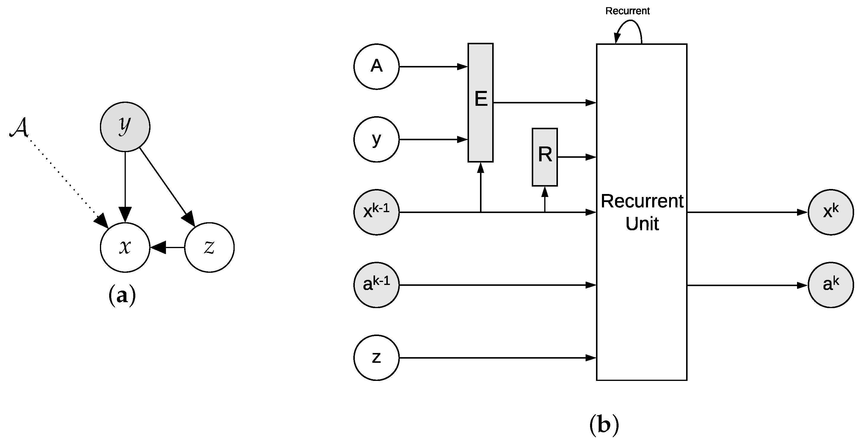
The graphical model is given in Figure 2a. The learning algorithm learns a conditional sampler, in a manner similar to a random number generator (RNG) for a given probability distribution. Note that for an RNG, different runs lead to different samples; but with a fixed random seed, the path is the same for different runs. The auxiliary (low-dimensional) latent variable z (conditionally dependent on the observation y) is an analogue of the random seed in the RNG, and is introduced into the deterministic recurrent process (modelled by a network) to diversify the reconstruction samples. In particular, for a fixed z, the recursion process inputs the sample initialization x 0 and applies a recurrent refining step based on suitable sample quality measures and the information encoded in the variable z.
Three DNNs are employed to model the distributions in L ( θ , ϕ ; x , y , A ) and to carry out the conditional sampling process, including one for the recursive process (i.e., recurrent unit modelled by a neural network) and two for probabilistic encoders (i.e., teacher and student encoders). The observation y and forward map A constitute their inputs: y is fed into the two probabilistic encoders and each recurrence of the recurrent unit; A is fed into each recurrence of the recurrent unit and the teacher encoder. Subsequently, we explain how the three networks work separately.
The recurrent component is the (deep) network h ϕ 2 ( · ) ; see Figure 2b. The network begins with an initial guess x 0 (default: back-projected data A * y ) and outputs x K after K iterations as the mean of p ϕ ( x | y , z , A ) , following the established idea of algorithmic unrolling [17,34], which mimics the iterations from standard optimization algorithms (e.g., (proximal) gradient descent, alternating direction method of multipliers (ADMM), and primal-dual hybrid gradient). At the k-th recursion, the network h ϕ 2 takes one sample x k 1 to refine and outputs an improved sample x k . To incorporate the forward map A and the observation y, we employ a functional E ( A , y , x k 1 ) . In the lens of variational regularisation [47], E ( A , y , x k 1 ) measures how well x k 1 can explain the data y. To indicate how well x k 1 fulfils the prior knowledge (e.g., sparsity and smoothness), we use the penalty R ( x k 1 ) as part of the input. For the sample quality measure E ( A , y , x k 1 ) and the penalty R ( x k 1 ) , we use | | y A ( x k 1 ) | | 2 (or its gradient), and | | x k 1 | | 2 2 or | x k 1 | TV (total variation semi-norm), respectively. Besides the latest iterate x k 1 and the quality measures E and R, the network h ϕ 2 ( · ) also takes a memory variable a k 1 and an auxiliary variable z. The memory variable a k 1 plays the role of momentum in gradient-type methods and is to retain long-term information between recursions. The overall procedure resembles an unrolled momentum accelerated gradient descent. The auxiliary random variable z is low-dimensional and injects randomness into the iteration procedure. Since both x k 1 and x k belong to the image space R n , we adopt CNNs without pooling layers to model the recurrent unit h ϕ 2 . Different inputs of h ϕ 2 ( · ) are concatenated along the channel axis, and the outputs of h ϕ 2 ( · ) —that is, the updated δ x k with x k = x k 1 + δ x k and the updated memory a k —are also concatenated.
Remark 3.
At each step, the recurrent unit (neural network h ϕ 2 ) reuses the observation data y and the map A for refinement, and the overall procedure differs from the deterministic mapping that serves as a post-processing step of back-projection. The latter is an end-to-end mapping that takes the back-projected data and outputs a refinement, but the proposed approach employs the current sample and quality measures and then decides the refinement strategy.
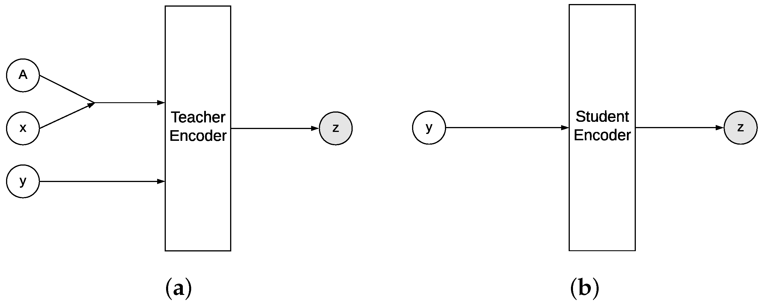
The framework employs two encoders of z: a teacher encoder q θ ( z | x , y , A ) and a student encoder p ϕ 1 ( z | y ) ; see Figure 3. The student encoder p ϕ 1 ( z | y ) takes the observation y, and encodes the observation-based knowledge so as to inform the recurrent unit h ϕ 2 . Given one sample z from p ϕ 1 ( z | y ) , the network h ϕ 2 gives one refining increment, and the distribution of z contributes to the diversity of the unknown image x. To help train the student encoder p ϕ 1 ( z | y ) , we provide the teacher encoder q θ ( z | x , y , A ) with the ground-truth x and the forward map A . The teacher encoder q θ ( z | x , y , A ) is discarded once the training is finished. The encoders p ϕ 1 ( z | y ) and q θ ( z | x , y , A ) are modelled by two DNNs h ϕ 1 ( · ) and h θ ( · ) , respectively, which reparameterise the auxiliary variable z. Since z is low-dimensional, CNNs with reduced mean layers and 1 × 1 convolutional layers can guarantee the flexibility dimension of the input y. To input the ground-truth data x and y into h θ ( · ) , we use the forward map A and concatenate A ( x ) with y along the channel axis. This construction is very flexible with the dimension problem and allows for the training of ( x i , y i ) of varying sizes (and the corresponding A i ).
Now we can state the complete algorithms for the training and inference of the cVAE framework for uncertainty-aware learned image reconstruction in Algorithms 1 and 2, respectively. Here, M denotes the mini-batch size, T the maximum number of training batches, K the number of recurrences of h ϕ 2 for one sample, and ( ϕ ^ , θ ^ ) the output of the training procedure (i.e., the learned parameters). There are many possible choices for the stochastic optimizer in line 11 of Algorithm 1 (e.g., ADAM [48], and SGD). We shall employ ADAM [48] in our experiment. The final sample from the recurrent process is regarded as the mean of the conditional distribution p ϕ ( x | y , z , A ) . Thus, given the initial x 0 , the iteration with different realisations of z leads to diverse samples of the unknown image x. Since each sample is the mean of p ϕ ( x | y , z , A ) rather than a direct sample from the approximate posterior p ϕ ( x | y ) , the summarizing statistics also have to be transformed; see (6). Note that the posterior variance contains two components: one is due to the background (i.e., β I ), and the other is due to the sample variance (i.e., 1 S i = 1 S x i x i t E ^ p ϕ ( x | y ) [ x ] E ^ p ϕ ( x | y ) [ x ] t ), as shown in the following result.
Algorithm 1 Training procedure
  1:
Input: Training data { ( x i , y i , A i ) } i = 1 N , β , T, K, M;
  2:
for t = 1 , 2 , , T do
  3:
 Randomly select a mini-batch training data { ( x i , y i , A i ) } i = 1 M ;
  4:
 Sample { z i } i = 1 M from { q θ ( z | x i , y i ) } i = 1 M ;
  5:
 Initialize { x ^ i } i = 1 M with { A i * ( y i ) } i = 1 M , and { a i } i = 1 M with zeros;
  6:
for k = 1 , 2 , , K do
  7:
  Update { x ^ i } i = 1 M and { a i } i = 1 M with { h ϕ 2 ( x ^ i , E ( A i , y i , x ^ i ) , R ( x ^ i ) , a i , z i ) } i = 1 M ;
  8:
end for
  9:
 Evaluate the KL divergence { D KL ( q θ ( z | x i , y i ) | | p ϕ 1 ( z | y i ) ) } i = 1 M ;
10:
 Compute the objective function L ^ ( ϕ , θ ) ;
11:
 Update the parameters ( ϕ , θ ) ;
12:
end for
13:
Output: ( ϕ ^ , θ ^ )
Algorithm 2 Inference procedure
  1:
Input: Test data ( A , y ) , S, K, ϕ ^ = ( ϕ 1 ^ , ϕ ^ 2 ) ;
  2:
for s = 1 , 2 , , S do
  3:
 Sample z s from p ϕ 1 ( z | y ) ;
  4:
 Initialise x ^ s with A * ( y ) and a with zeros;
  5:
for k = 1 , 2 , , K do
  6:
  Update x ^ s and a with h ϕ 2 ( x ^ s , E ( A , y , x ^ s ) , R ( x ^ s ) , a , z s ) ;
  7:
end for
  8:
end for
  9:
Output: { x ^ s } s = 1 S ;
10:
Evaluate ( E ^ p ( x | y ) [ x ] , Cov ^ p ( x | y ) [ x ] ) by Equation (6)
Proposition 2.
Let p ϕ ( x | y , z , A ) = N ( x | x K ( z ) , β I ) and the approximate posterior p ϕ ( x | y ) = p ϕ 2 ( x | y , z , A ) p ϕ 1 ( z | y ) d z be a mixture of Gaussian distributions, with z being the mixture variable. Then, given samples { z i } i = 1 S of z from p ϕ ( z | y ) , and the corresponding x K ( z ) denoted by { x i } i = 1 S , the mean E p ϕ ( x | y ) [ x ] and the covariance Cov p ϕ ( x | y ) [ x ] of p ϕ ( x | y ) can be estimated by:
E ^ p ϕ ( x | y ) [ x ] = 1 S i = 1 S x i , Cov ^ p ϕ ( x | y ) [ x ] = β I + 1 S i = 1 S x i x i t E ^ p ϕ ( x | y ) [ x ] E ^ p ϕ ( x | y ) [ x ] t .
Proof. 
For the mean E p ϕ ( x | y ) [ x ] , by dentition, there holds the following:
E p ϕ ( x | y ) [ x ] = x x p ϕ ( x | y ) d x = x x z p ϕ 2 ( x | y , z , A ) p ϕ 1 ( z | y ) d z d x = z x x p ϕ 2 ( x | y , z , A ) d x p ϕ 1 ( z | y ) d z = z x K ( z ) p ϕ 1 ( z | y ) d z .
Thus, 1 S i = 1 S x i is an unbiased estimator of E p ϕ ( x | y ) [ x ] . Similarly, for the covariance Cov p ϕ ( x | y ) [ x ] , by the standard bias variance decomposition,
Cov p ϕ ( x | y ) [ x ] = x x T p ϕ ( x | y ) d x E p ϕ ( x | y ) [ x ] E p ϕ ( x | y ) [ x ] T .
Now, the first term on the right hand side, there holds the following:
x x T p ϕ ( x | y ) d x = x x x T z p ϕ 2 ( x | y , z , A ) p ϕ 1 ( z | y ) d z d x = z x x x T p ϕ 2 ( x | y , z , A ) d x p ϕ 1 ( z | y ) d z = z ( Cov p ϕ 2 ( x | y , z , A ) [ x ] + E p ϕ 2 ( x | y , z , A ) [ x ] E p ϕ 2 ( x | y , z , A ) [ x ] T ) p ϕ 1 ( z | y ) d z = β I + z E p ϕ 2 ( x | y , z , A ) [ x ] E p ϕ 2 ( x | y , z , A ) [ x ] T p ϕ 1 ( z | y ) d z .
Consequently, β I + 1 S i = 1 S x i x i t E ^ p ϕ ( x | y ) [ x ] E ^ p ϕ ( x | y ) [ x ] t is an unbiased estimator of the covariance Cov p ϕ ( x | y ) [ x ] .    □

5. Numerical Experiments and Discussions

Now we showcase the proposed cVAE framework for learned reconstruction with quantified aleatoric uncertainty with numerical experiments on positron emission tomography (PET). PET is a pillar of modern diagnostic imaging, allowing for non-invasive, sensitive, and specific detection of functional changes in a number of diseases. Most conventional PET reconstruction algorithms rely on penalized maximum likelihood estimates, using a hand crafted prior (e.g., total variation and anatomical); see the work of [28] for an overview of classical reconstruction techniques. More recently, learning-based approaches have been proposed. While these techniques have been successful, they still lack the capability to provide uncertainty estimates; see the work of [29,30,31,37] for several recent studies on UQ in PET reconstruction, although none of them is based on deep learning.
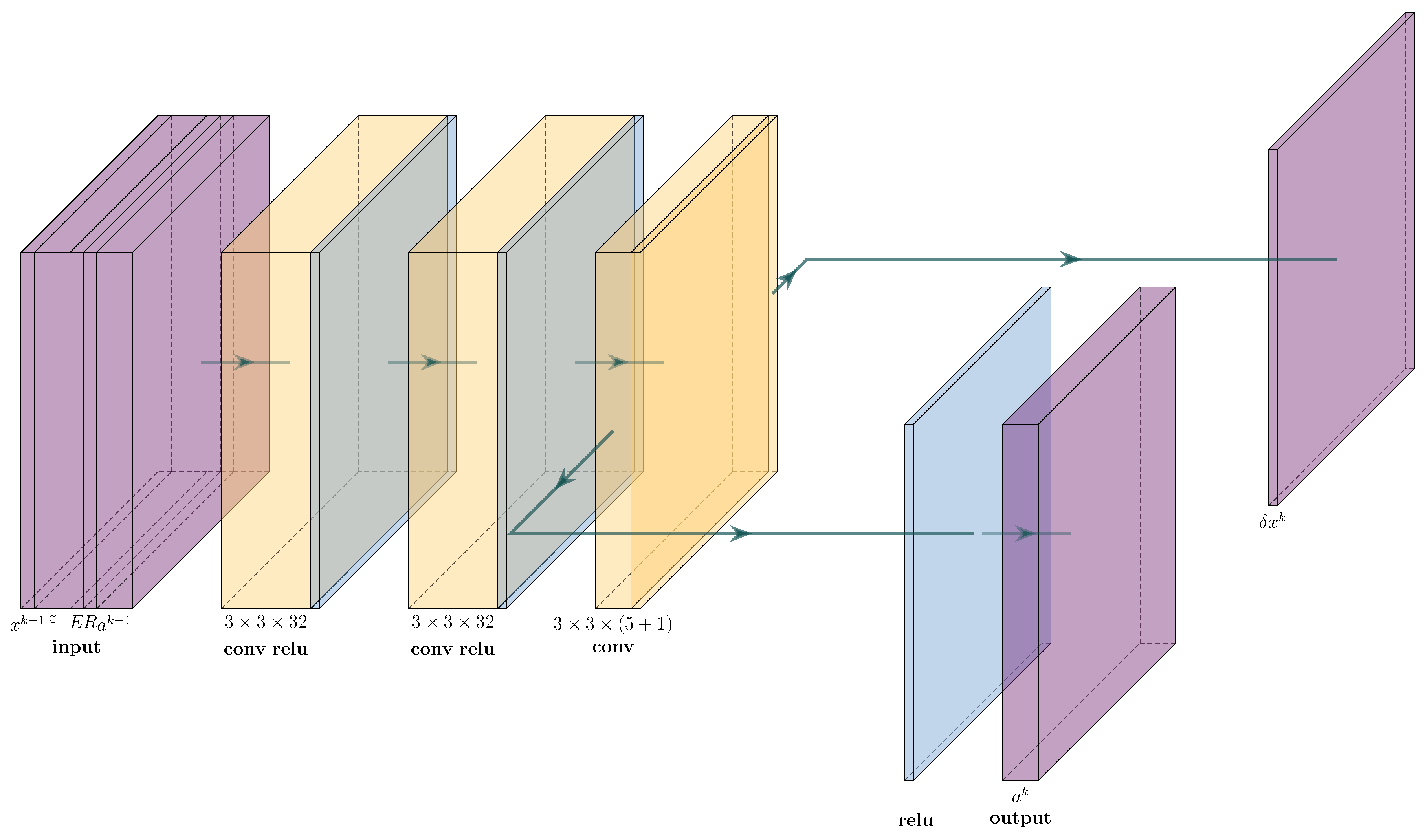
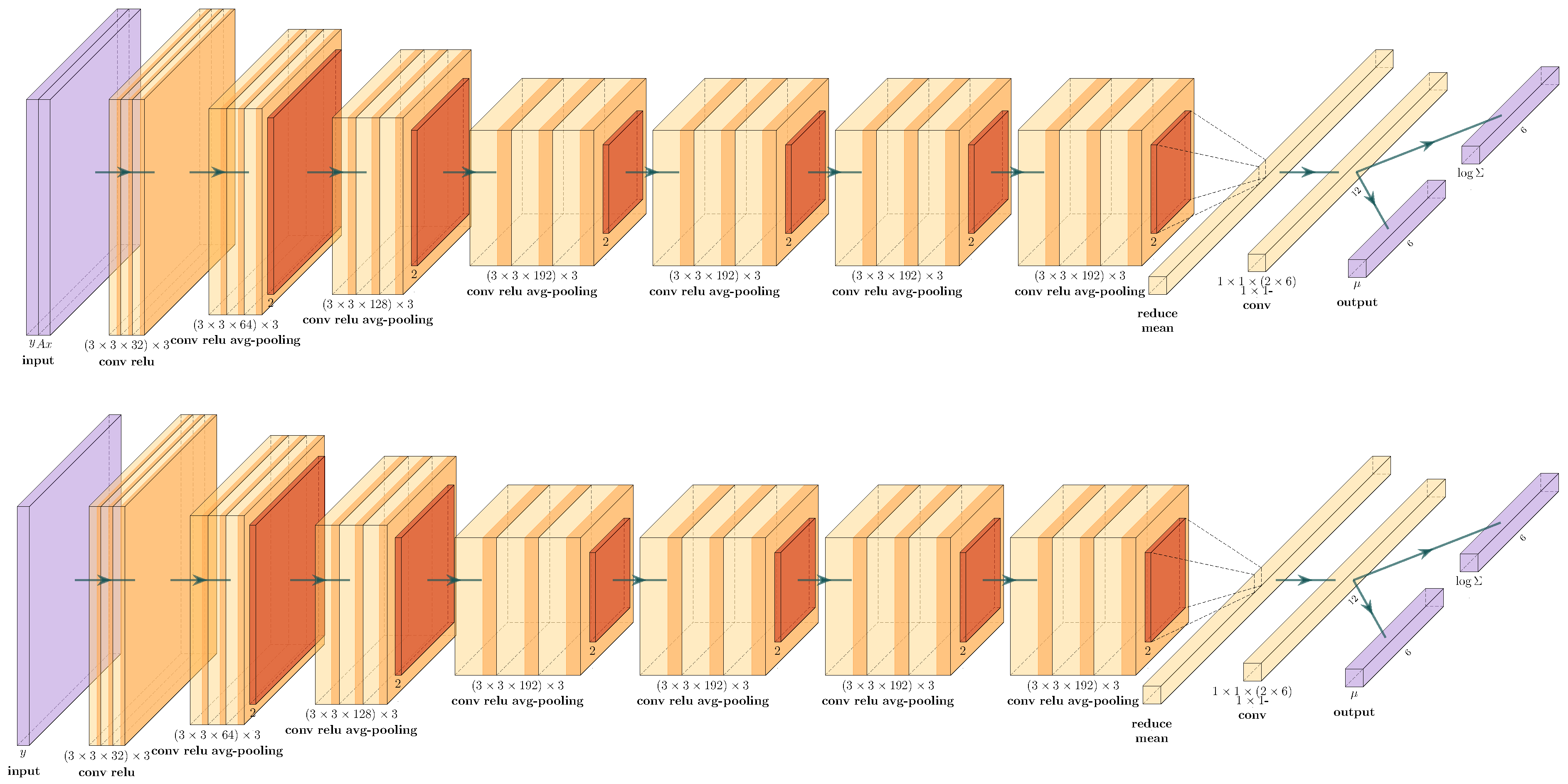
For the experiments below, we employ a three-layer CNN as the recurrent unit h ϕ 2 and fix K = 10 iterations for each sampling step, cf. Figure 4 for a schematic illustration; VGG style encoders are then used for both h ϕ 1 and h θ , cf. Figure 5. We train the network on a synthetic dataset consisting of elliptical phantoms and test it on the public medical imaging dataset BrainWeb [49] (available from https://brainweb.bic.mni.mcgill.ca/, last accessed on 10 January 2020). Throughout, the training pair ( x , y ) R 128 × 128 × R 30 × 183 , and the forward map is the Radon transform, which is normalised. Different peak values of x are used to indicate the count level: 1 × 10 4 and 1 × 10 2 for respectively moderate and low count levels. The observation y is generated by corrupting the sinogram A x by Poisson noise entrywise, i.e., y i Pois ( ( A x ) i ) , where Pois ( · ) denotes the Poisson random variable. The hyper-parameter β is tuned in a trial-and-error manner and fixed at β = 5 × 10 3 below. The experiments are conducted on a desktop with two Nvidia GeForce 1080 Ti GPUs and Intel i7-7700K CPU 4.20GHz×8. It is trained for T = 1 × 10 5 batches, each of which contains 10 randomly generated ( x , y ) pairs on-the-fly. The training almost converges after 2 × 10 4 batches, and it takes around 11 hours to go over all T = 1 × 10 5 batches. The summarizing statistics reported below are computed from 1000 samples for each observation y generated by the trained network. The implementation uses the following public deep learning frameworks: Tensorflow (https://www.tensorflow.org/, [50]), Tensorflow Probability (https://www.tensorflow.org/probability, 51]), DeepMind Sonnet (github.com/deepmind/sonnet), and ODL (github.com/odlgroup/odl), all last accessed on 10 January 2020; the source code will be made available at github.com/chenzxyz/cvae accessed on 10 January 2020.
First, we compare the proposed cVAE approach with conventional and deep learning-based methods on all 181 phantoms in the BrainWeb dataset. It is compared with the following three benchmark methods: maximum likelihood EM (MLEM) [52], total variation (TV) [53] with non-negativity constraint, and learned gradient descent (LGD) [54]. MLEM and TV are two established reconstruction methods in the PET community, and LGD is an unrolled iterative method inspired by classical variational regularisation and exploit DNNs for iterative refinement. For MLEM, we use the odl inbuilt solver mlem, and for TV, we use the primal dual hybrid gradient method (implemented by odl.solvers.phgd). The regularisation parameter α for total variation prior is fixed at α = 2 × 10 1 and α = 2 for the moderate and low count levels, respectively, which is determined in a trial-and-error manner. The comparative results are summarised in Table 1, shown with two of the most popular image quality metrics, i.e., SSIM and PSNR, averaged over all 181 phantoms in the BrainWeb dataset. The results clearly show that cVAE can deliver state-of-the-art point estimates in terms of PSNR and SSIM, especially in the practically very important low-count case. Compared with these deterministic benchmark methods, cVAE can additionally provide information on uncertainty.
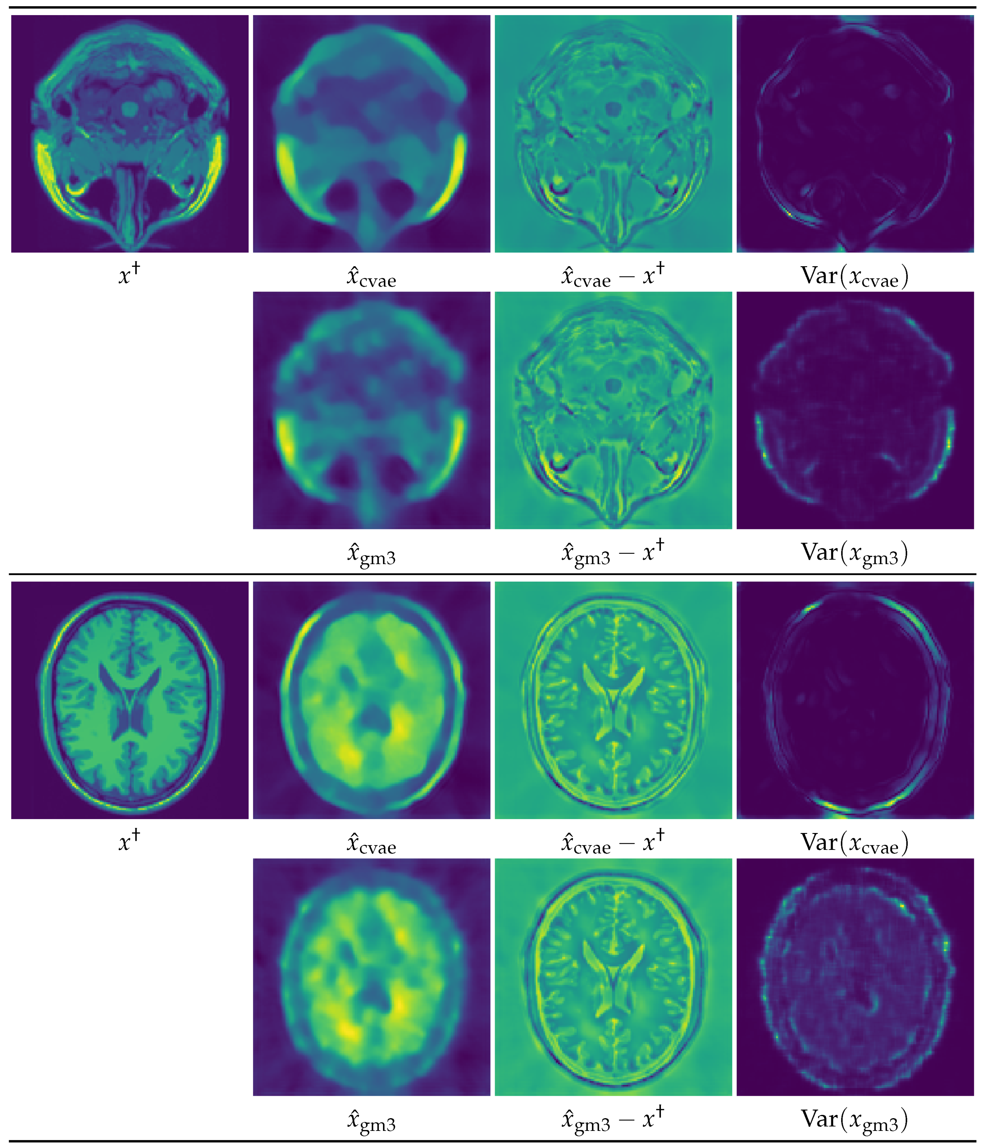
Next, we compare cVAE with a probabilistic approach [19], which reports state-of-the-art performance for aleatoric uncertainty (see [55] for theoretical interpretations). It employs (non-Bayesian) neural network ensembles to estimate predictive uncertainty, where each network in the ensemble learns similar values close to the training data, and different ones in regions of the space far from the training data. For the comparison, we train a mixture with three multivariate Gaussians (GM3) without adversarial samples, where the training of each component of the mixture is to fit a mean network and a variance network of the outputs using a Gaussian log-likelihood [56]. To stabilize the training procedure, we first train the mean network, and then train the variance network. Alternatively, one can train the mean network as a warm up and then train the mean and variance networks simultaneously, but it usually leads to worse results, and thus we do not present the corresponding results. The comparative quantitative results are given in Table 2, which present the PSNR and SSIM results for ten phantoms from the Brainweb dataset in order to shed fine-grained insights into the performance of the methods over different phantoms. It is observed that in the low count case, cVAE can provide better point estimates in terms of both SSIM and PSNR, which concurs with Figure 6; however, in the moderate count case, GM3 can sometimes deliver better results. In terms of the variance map, the results of GM3 contain more structural patterns and resemble the error map more closely.
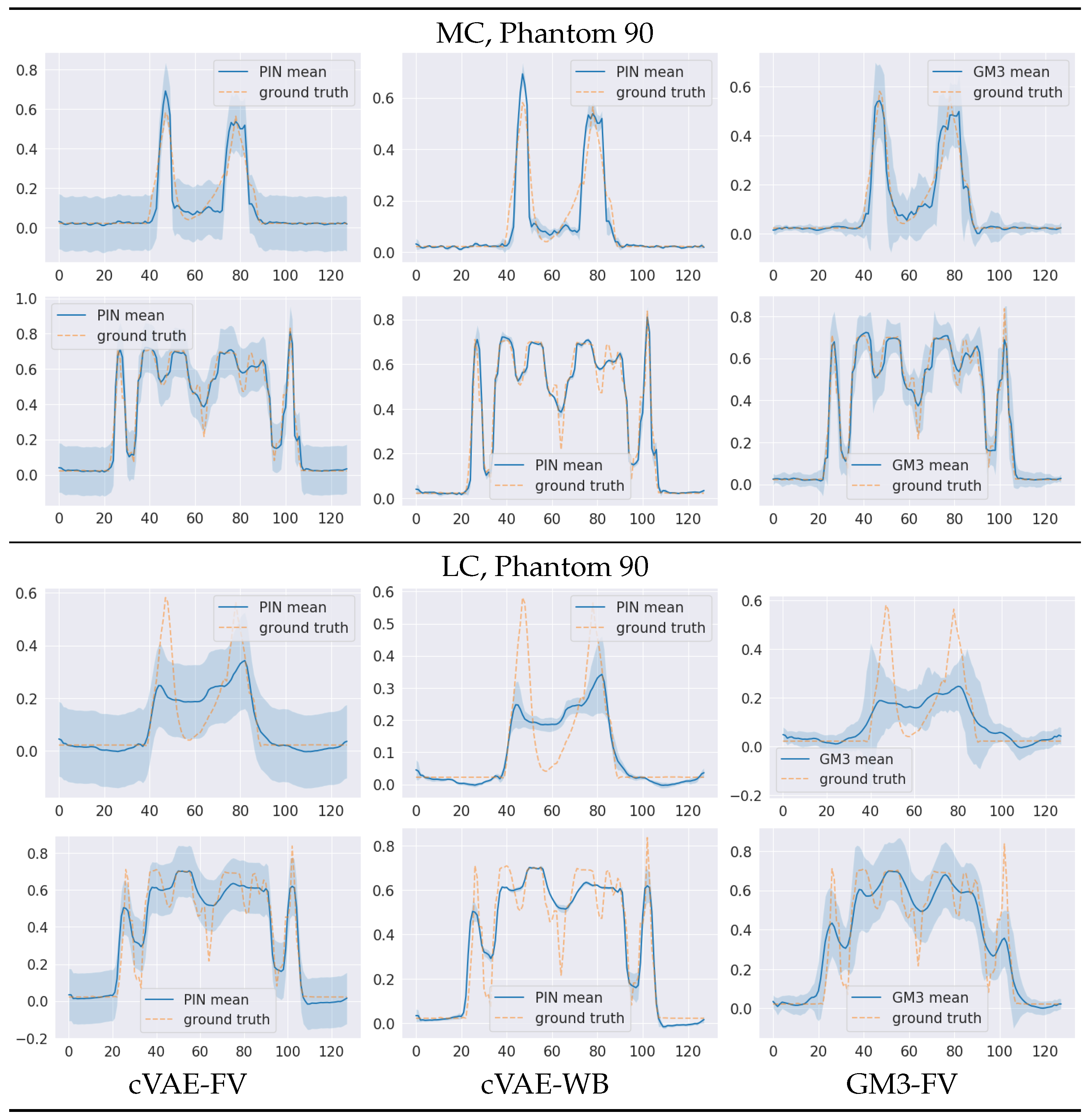
To shed more insights into the variance by cVAE and the benchmark GM3, we show the cross-section plots with 0.95 Highest Posterior Density (HPD) in Figure 7 for both moderate and low count levels. According to Proposition 2, the estimated covariance by cVAE contains two distinct sources, i.e., the sample variance and the variance β of the conditional Gaussians p ϕ ( x | y , z , A ) = N ( x | x K ( z ) , β I ) . The latter is uniform across the pixels and acts as a background. We show the HPDs of cVAE with full variance (unbiased variance estimated by Cov ^ p ϕ ( x | y ) [ x ] ) and the variance without the β factor (i.e., Cov ^ p ϕ ( x | y ) [ x ] β I ). It is observed that the latter contains more structures in the credible intervals. Furthermore, the overall shape and magnitude of the HPDs by cVAE with the full variance and GM3 are fairly close to each other. It is noteworthy that in the cold regions (i.e., zero count), cVAE can provide almost zero variance upon subtracting the background variance, and it is able to indicate the contrast of variance to highlight the pixels, whereas the variances by GM3 are also relatively high. The comparison between the cross-section plots for low and moderate count cases (i.e., high and low noise levels) on the same ground-truth phantom indicates that cVAE does provide higher uncertainty for a higher noise level, which is intuitively consistent with the underlying statistical background.
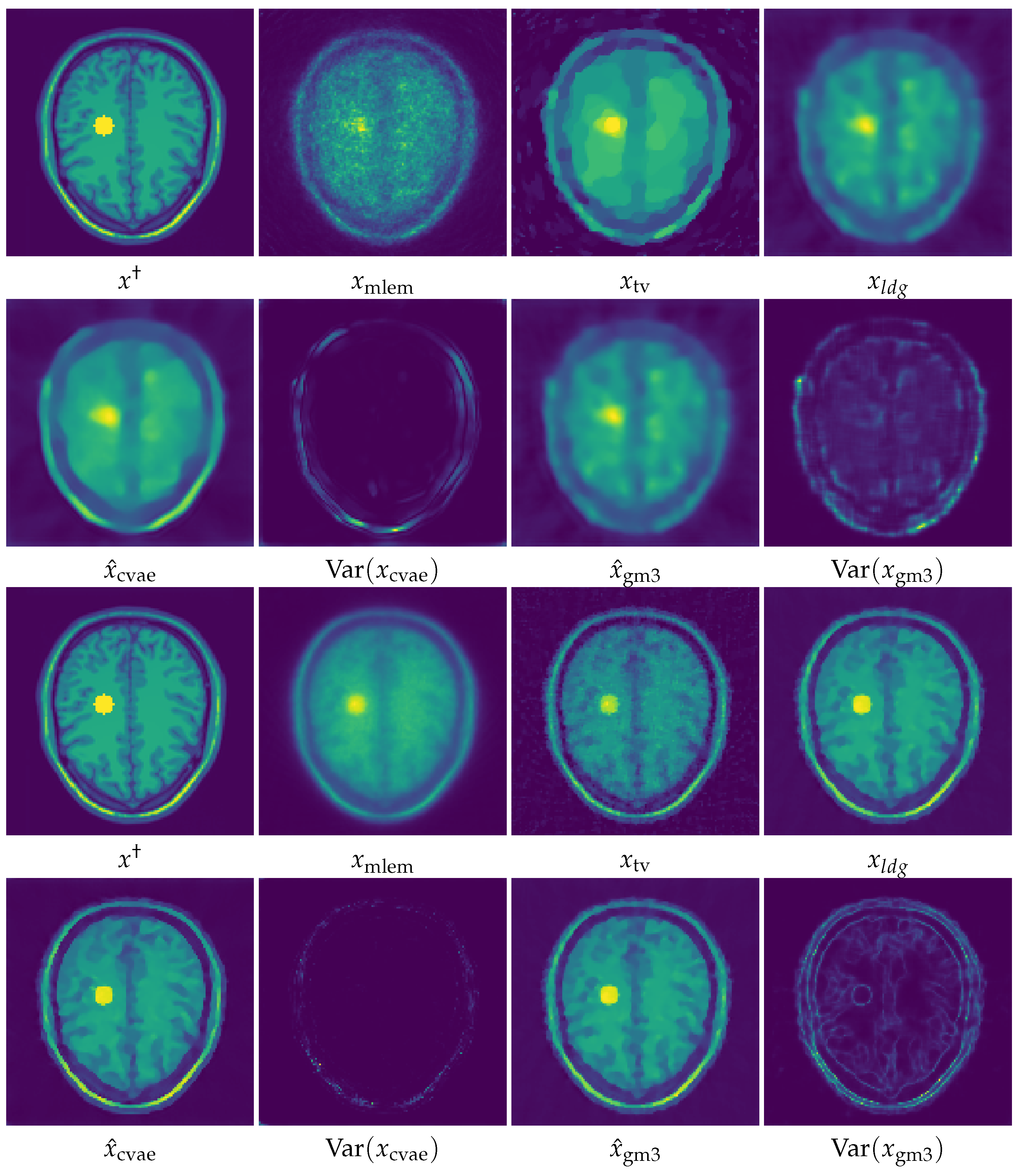
Lastly, we evaluate all the methods on the phantoms with an artificially added tumour by changing the pixel values to the peak values in order to examine their capability of recovering novel features that are not presented in the training data. We (randomly) choose two phantoms from the BrainWeb dataset (Python style index: 10 and 110). A small tumour with a radius of 2 and a large tumour with a radius of 5 are added into the 10th and 110th phantoms, respectively. The corresponding reconstructions are shown in Figure 8 and Figure 9, respectively. It is observed that the tumours can be clearly reconstructed by the cVAE means for both count levels, except for the small tumour at low count levels. In the latter case, none of the methods can reasonably reconstruct the tumour since the data are very noisy in terms of low signal strength. The results by cVAE, LGD, and GM3 are comparable, at least visually. The ability to reconstruct tumours further indicates that cVAE does not miss out on important features that are not present in the training data, indicating a certain degree of robustness of the cVAE framework, so long as the signal is sufficiently strong, since many deep learning-based methods tend to miss the tumour due to the bias induced by tumour-free training data [57].

6. Conclusions

In this work, we have developed a general and flexible probabilistic computational framework for the uncertainty quantification of inverse problems in a purely data-driven setting. The approach is based on the conditional variational autoencoder loss and employs the deep neural network as a recurrent unit to repeatedly refine the samples using the observation and forward map, seeded by a probabilistic encoder conditioned on the observation. The efficiency of the framework is underpinned by the encoding of observations in a low-dimensional latent space. The significant potentials of the framework have been demonstrated on a PET image reconstruction with both moderate and low count levels, and the approach shows competitive performance when compared with several deterministic and probabilistic benchmark methods, especially within the low count regime.
There are several avenues for further study. First, the framework is flexible and general, and it is of much interest to evaluate its potentials on other computationally expensive imaging modalities (e.g., MRI, CT, and PET-MRI), especially in the under sampling and low-dose regime, for which there is a great demand on uncertainty quantification due to the lack of sufficient information. Such studies will also provide important insights into the statistical features of the framework. Second, it is of much interest to analyse the theoretical properties of the cVAE loss as an upper bound of the expected KL divergence (e.g., approximation error and asymptotic convergence). This line of research has long been outstanding in approximate inference and often provides theoretical guarantees for the overall inference procedure and guidelines for constructing efficient approximations. Third and last, it is imperative to develop scalable benchmarks for the uncertainty quantification of high-dimensional inverse problems. Several deep learning-based uncertainty quantification techniques have been proposed in the machine learning literature, but mostly on different types of uncertainties or without explicitly elucidating the sources of uncertainties (see the work of [25] for a preliminary study in medical imaging). A careful calibration of the obtained uncertainties is essential towards practical deployment, as recently highlighted in the review presented in [8].

Author Contributions

Conceptualization, C.Z. and B.J.; methodology, C.Z. and B.J.; investigation, C.Z. and R.B.; writing C.Z., R.B., and B.J.; supervision, B.J.; project administration, B.J.; funding acquisition, B.J. All authors have read and agreed to the published version of the manuscript.

Funding

The work of B.J. is partly supported by UK EPSRC EP/T000864/1.

Institutional Review Board Statement

Not applicable.

Informed Consent Statement

Not applicable.

Data Availability Statement

The study did not report any data.

Conflicts of Interest

The authors declare no conflict of interest.

References

  1. Zhang, K.; Zuo, W.; Chen, Y.; Meng, D.; Zhang, L. Beyond a Gaussian denoiser: Residual learning of deep CNN for image denoising. IEEE Trans. Imag. Proc. 2017, 26, 3142–3155. [Google Scholar] [CrossRef] [Green Version]
  2. Xu, L.; Ren, J.S.; Liu, C.; Jia, J. Deep convolutional neural network for image deconvolution. In Advances in Neural Information Processing Systems; MIT Press: Cambridge, MA, USA, 2014; pp. 1790–1798. [Google Scholar]
  3. Dong, C.; Loy, C.C.; He, K.; Tang, X. Learning a deep convolutional network for image super-resolution. In Proceedings of the ECCV 2014: Computer Vision, Zurich, Switzerland, 6–12 September 2014; pp. 184–199. [Google Scholar]
  4. Kang, E.; Min, J.; Ye, J.C. A deep convolutional neural network using directional wavelets for low-dose X-ray CT reconstruction. Med. Phys. 2017, 44, e360–e375. [Google Scholar] [CrossRef] [Green Version]
  5. Chen, H.; Zhang, Y.; Chen, Y.; Zhang, J.; Zhang, W.; Sun, H.; Lv, Y.; Liao, P.; Zhou, J.; Wang, G. LEARN: Learned experts’ assessment-based reconstruction network for sparse-data CT. IEEE Trans. Med. Imag. 2018, 37, 1333–1347. [Google Scholar] [CrossRef]
  6. Hyun, C.M.; Kim, H.P.; Lee, S.M.; Lee, S.; Seo, J.K. Deep learning for undersampled MRI reconstruction. Phys. Med. Biol. 2018, 63, 135007. [Google Scholar] [CrossRef]
  7. Kendall, A.; Gal, Y. What uncertainties do we need in Bayesian deep learning for computer vision? In Advances in Neural Information Processing Systems; Curran Associates Inc.: Red Hook, NY, USA, 2017; pp. 5574–5584. [Google Scholar]
  8. Barbano, R.; Arridge, S.; Jin, B.; Tanno, R. Uncertainty quantification in medical image synthesis. In Biomedical Image Synthesis and Simulations: Methods and Applications; Burgos, N., Svoboda, D., Eds.; Elsevier: Amsterdam, The Netherlands, 2022; in press. [Google Scholar]
  9. Kaipio, J.; Somersalo, E. Statistical and Computational Inverse Problems; Springer: New York, NY, USA, 2005; p. xvi+339. [Google Scholar]
  10. Stuart, A.M. Inverse problems: A Bayesian perspective. Acta Numer. 2010, 19, 451–559. [Google Scholar] [CrossRef] [Green Version]
  11. Arjovsky, M.; Chintala, S.; Bottou, L. Wasserstein GAN. arXiv 2017, arXiv:1701.07875. [Google Scholar]
  12. Kingma, D.P.; Welling, M. Auto-encoding variational bayes. arXiv 2013, arXiv:1312.6114. [Google Scholar]
  13. Borcea, L. Electrical impedance tomography. Inverse Probl. 2002, 18, R99–R136. [Google Scholar] [CrossRef]
  14. Arridge, S.R.; Schotland, J.C. Optical tomography: Forward and inverse problems. Inverse Probl. 2009, 25, 123010. [Google Scholar] [CrossRef]
  15. Zhang, C.; Jin, B. Probabilistic residual learning for aleatoric uncertainty in image restoration. arXiv 2019, arXiv:1908.01010. [Google Scholar]
  16. Sohn, K.; Lee, H.; Yan, X. Learning structured output representation using deep conditional generative models. In Advances in Neural Information Processing Systems; MIT Press: Cambridge, MA, USA, 2015; pp. 3483–3491. [Google Scholar]
  17. Monga, V.; Li, Y.; Eldar, Y.C. Algorithm unrolling: Interpretable, efficient deep learning for signal and image processing. IEEE Signal Proc. Mag. 2021, 38, 18–44. [Google Scholar] [CrossRef]
  18. Wainwright, M.J.; Jordan, M.I. Graphical models, exponential families, and variational inference. Found. Trends Mach. Learn. 2008, 1, 1–305. [Google Scholar] [CrossRef] [Green Version]
  19. Lakshminarayanan, B.; Pritzel, A.; Blundell, C. Simple and scalable predictive uncertainty estimation using deep ensembles. In Advances in Neural Information Processing Systems; Curran Associates Inc.: Red Hook, NY, USA, 2017; pp. 6402–6413. [Google Scholar]
  20. Gal, Y.; Ghahramani, Z. Dropout as a Bayesian approximation: Representing model uncertainty in deep learning. In Proceedings of the 33rd International Conference on Machine Learning, New York, NY, USA, 20–22 June 2016; pp. 1050–1059. [Google Scholar]
  21. Abdar, M.; Pourpanah, F.; Hussain, S.; Rezazadegan, D.; Liu, L.; Ghavamzadeh, M.; Fieguth, P.; Khosravi, A.; Acharya, U.R.; Makarenkov, V.; et al. A review of uncertainty quantification in deep learning: Techniques, applications and challenges. Inf. Fusion 2021, 76, 243–297. [Google Scholar] [CrossRef]
  22. Graves, A. Practical variational inference for neural networks. In Advances in Neural Information and Processing Systems; Curran Associates Inc.: Red Hook, NY, USA, 2011; pp. 2348–2356. [Google Scholar]
  23. Blundell, C.; Cornebise, J.; Kavukcuoglu, K.; Wierstra, D. Weight uncertainty in neural network. In Proceedings of the International Conference on Machine Learning, Lille, France, 7–9 July 2015; pp. 1613–1622. [Google Scholar]
  24. Barbano, R.; Zhang, C.; Arridge, S.; Jin, B. Quantifying model uncertainty in inverse problems via Bayesian deep gradient descent. In Proceedings of the 25th International Conference on Pattern Recognition (ICPR), Milan, Italy, 10–15 January 2021; pp. 1392–1399. [Google Scholar]
  25. Barbano, R.; Kereta, Z.; Zhang, C.; Hauptmann, A.; Arridge, S.; Jin, B. Quantifying sources of uncertainty in deep learning-based image reconstruction. arXiv 2020, arXiv:2011.08413v2. [Google Scholar]
  26. Minka, T.P. Expectation propagation for approximate Bayesian inference. arXiv 2013, arXiv:1301.2294. [Google Scholar]
  27. Osawa, K.; Swaroop, S.; Jain, A.; Eschenhagen, R.; Turner, R.E.; Yokota, R.; Khan, M.E. Practical deep learning with Bayesian principles. arXiv 2019, arXiv:1906.02506v2. [Google Scholar]
  28. Qi, J.; Leahy, R.M. Iterative reconstruction techniques in emission computed tomography. Phys. Med. Biol. 2006, 51, R541–R578. [Google Scholar] [CrossRef]
  29. Zhang, C.; Arridge, S.R.; Jin, B. Expectation Propagation for Poisson Data. Inverse Probl. 2019, 35, 085006. [Google Scholar] [CrossRef] [Green Version]
  30. Filipović, M.; Barat, E.; Dautremer, T.; Comtat, C.; Stute, S. PET reconstruction of the posterior image probability, including multimodal images. IEEE Trans. Med. Imag. 2019, 38, 1643–1654. [Google Scholar] [CrossRef]
  31. Zhou, Q.; Yu, T.; Zhang, X.; Li, J. Bayesian inference and uncertainty quantification for medical image reconstruction with Poisson data. SIAM J. Imaging Sci. 2020, 13, 29–52. [Google Scholar] [CrossRef]
  32. Ongie, G.; Jalal, A.; Baraniuk, R.G.; Metzler, C.A.; Dimakis, A.G.; Willett, R. Deep learning techniques for inverse problems in imaging. IEEE J. Sel. Areas Inform. Theory 2020, 1, 39–56. [Google Scholar] [CrossRef]
  33. Gregor, K.; LeCun, Y. Learning fast approximations of sparse coding. In Proceedings of the International Conference on Machine Learning, Haifa, Israel, 21–24 June 2010; pp. 1–8. [Google Scholar]
  34. Putzky, P.; Welling, M. Recurrent inference machines for solving inverse problems. arXiv 2017, arXiv:1706.04008. [Google Scholar]
  35. Jordan, M.I.; Ghahramani, Z.; Jaakkola, T.S.; Saul, L.K. An introduction to variational methods for graphical models. Mach. Learn. 1999, 37, 183–233. [Google Scholar] [CrossRef]
  36. Opper, M.; Archambeau, C. The variational Gaussian approximation revisited. Neural Comput. 2009, 21, 786–792. [Google Scholar] [CrossRef]
  37. Arridge, S.R.; Ito, K.; Jin, B.; Zhang, C. Variational Gaussian approximation for Poisson data. Inverse Probl. 2018, 34, 025005. [Google Scholar] [CrossRef]
  38. MacKay, D.J.C. Information Theory, Inference and Learning Algorithms; Cambridge University Press: Cambridge, UK, 2003. [Google Scholar]
  39. Chai, Y.; Liu, M.; Duffy, B.A.; Kim, H. Learning to Synthesize cortical morphological changes using graph conditional variational autoencoder. In Proceedings of the 2021 IEEE 18th International Symposium on Biomedical Imaging (ISBI), Nice, France, 13–16 April 2021. [Google Scholar] [CrossRef]
  40. Hou, T.Y.; Lam, K.C.; Zhang, P.; Zhang, S. Solving Bayesian inverse problems from the perspective of deep generative networks. Comput. Mech. 2019, 64, 395–408. [Google Scholar] [CrossRef]
  41. Kullback, S.; Leibler, R.A. On information and sufficiency. Ann. Math. Stat. 1951, 22, 79–86. [Google Scholar] [CrossRef]
  42. Rezende, D.J.; Mohamed, S.; Wierstra, D. Stochastic backpropagation and approximate inference in deep generative models. In Proceedings of the 31st International Conference on International Conference on Machine Learning, Beijing, China, 21–26 June 2014; Volume 32, pp. 1278–1286. [Google Scholar]
  43. Kingma, D.P.; Welling, M. An introduction to variational autoencoders. arXiv 2019, arXiv:1906.02691. [Google Scholar] [CrossRef]
  44. Khemakhem, I.; Kingma, D.; Monti, R.; Hyvarinen, A. Variational autoencoders and nonlinear ica: A unifying framework. In Proceedings of the International Conference on Artificial Intelligence and Statistics, PMLR, Palermo, Italy, 3–5 June 2020; pp. 2207–2217. [Google Scholar]
  45. Walker, J.; Doersch, C.; Gupta, A.; Hebert, M. An uncertain future: Forecasting from static images using variational autoencoders. In Proceedings of the European Conference on Computer Vision, Amsterdam, The Netherlands, 11–14 October 2016; pp. 835–851. [Google Scholar]
  46. Liu, J.S. Monte Carlo Strategies in Scientific Computing; Springer: New York, NY, USA, 2001; p. xvi+343. [Google Scholar]
  47. Ito, K.; Jin, B. Inverse Problems: Tikhonov Theory and Algorithms; World Scientific Publishing Co. Pte. Ltd.: Hackensack, NJ, USA, 2015; p. x+318. [Google Scholar]
  48. Kingma, D.P.; Ba, J. Adam: A method for stochastic optimization. In Proceedings of the 3rd International Conference on Learning Representations (ICLR), San Diego, CA, USA, 7–9 May 2015. [Google Scholar]
  49. Cocosco, C.A.; Kollokian, V.; Kwan, R.K.S.; Pike, G.B.; Evans, A.C. Brainweb: Online interface to a 3D MRI simulated brain database. NeuroImage 1997, 5, S425. [Google Scholar]
  50. Abadi, M.; Barham, P.; Chen, J.; Chen, Z.; Davis, A.; Dean, J.; Devin, M.; Ghemawat, S.; Irving, G.; Isard, M.; et al. Tensorflow: A system for large-scale machine learning. In Proceedings of the 12th USENIX Symposium on Operating Systems Design and Implementation (OSDI 16), Savannah, GA, USA, 2–4 November 2016; pp. 265–283. [Google Scholar]
  51. Dillon, J.V.; Langmore, I.; Tran, D.; Brevdo, E.; Vasudevan, S.; Moore, D.; Patton, B.; Alemi, A.; Hoffman, M.; Saurous, R.A. Tensorflow distributions. arXiv 2017, arXiv:1711.10604. [Google Scholar]
  52. Shepp, L.A.; Vardi, Y. Maximum likelihood reconstruction for emission tomography. IEEE Trans. Med. Imag. 1982, 1, 113–122. [Google Scholar] [CrossRef] [PubMed]
  53. Rudin, L.I.; Osher, S.; Fatemi, E. Nonlinear total variation based noise removal algorithms. Phys. D. Nonlinear Phenom. 1992, 60, 259–268. [Google Scholar] [CrossRef]
  54. Adler, J.; Öktem, O. Solving ill-posed inverse problems using iterative deep neural networks. Inverse Probl. 2017, 33, 124007. [Google Scholar] [CrossRef] [Green Version]
  55. He, B.; Lakshminarayanan, B.; Teh, Y.W. Bayesian deep ensembles via the neural tangent kernel. arXiv 2020, arXiv:2007.05864. [Google Scholar]
  56. Nix, D.A.; Weigend, A.S. Estimating the mean and variance of the target probability distribution. In Proceedings of the 1994 IEEE International Conference on Neural Networks (ICNN’94), Orlando, FL, USA, 28 June–2 July 1994; Volume 1, pp. 55–60. [Google Scholar]
  57. Moeller, M.; Möllenhoff, T.; Cremers, D. Controlling neural networks via energy dissipation. arXiv 2019, arXiv:1904.03081. [Google Scholar]
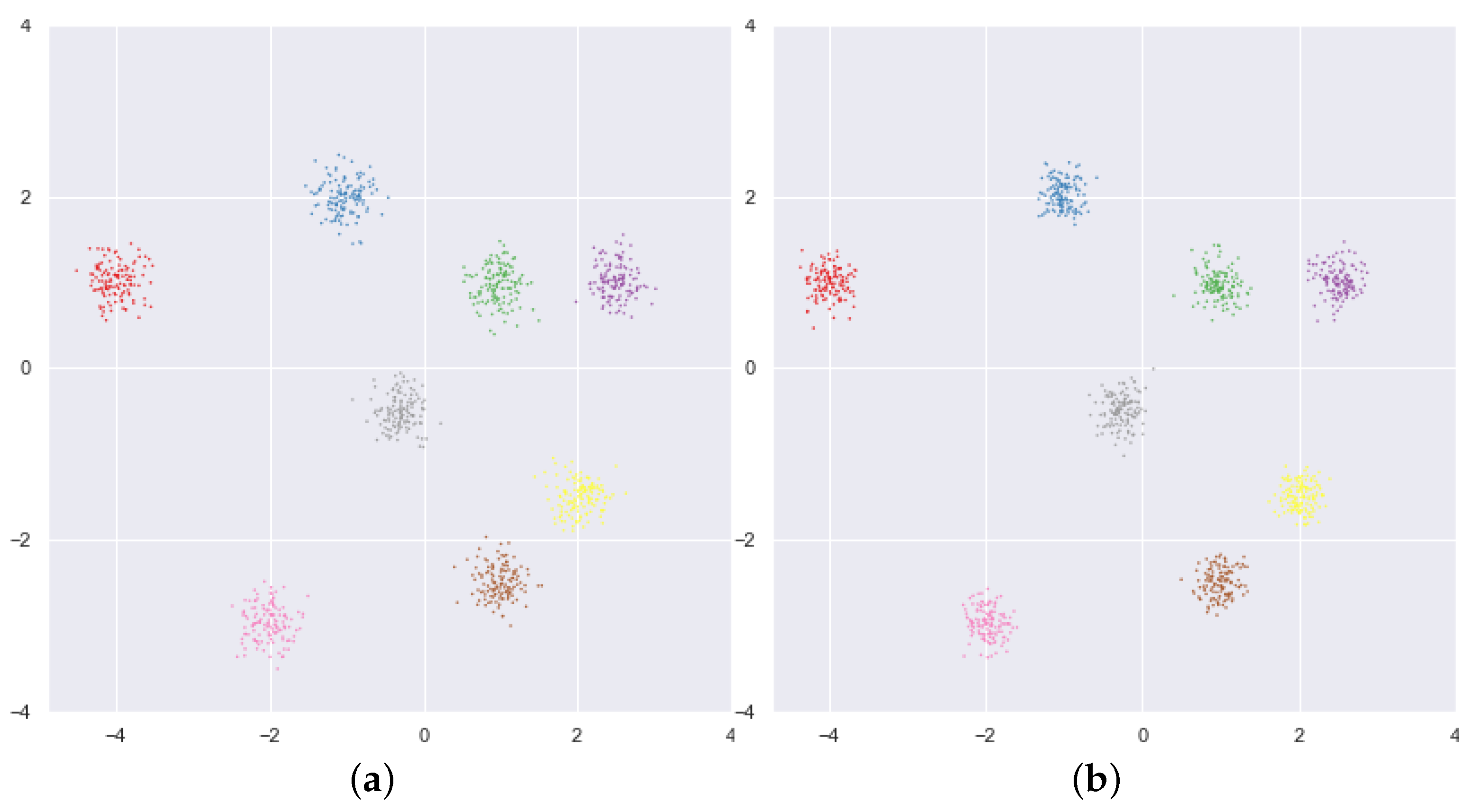
Figure 1. Validation of the cVAE for a toy two-dimensional distribution and Gaussian mixture with eight components. (a) Ground-truth; (b) cVAE approximation.
Computation 09 00114 g001
Figure 2. The graphical model and recurrent network of cVAE. (a) Graphical model. Shaded and non-shaded nodes denote observations and hidden variables, respectively; solid and dotted arrows denote probabilistic dependencies and explicit incorporations, respectively. (b) Recurrent network h ϕ 2 . Shaded and non-shaded circles denote variables for updating and fixed ones, respectively; shaded rectangles denote functional input. For each fixed z, only the values of shaded objects change.
Computation 09 00114 g002
Figure 3. Probabilistic encoders in the framework. Shaded nodes denote the random variable. (a) Teacher encoder q θ ( z | x , y , A ) . (b) Student encoder p ϕ 1 ( z | y ) .
Computation 09 00114 g003
Figure 4. The layer configuration of the recurrent unit h ϕ 2 : 3 × 3 × 32 denotes a convolutional layer with a kernel size of 3 × 3 and 32 output channels. In the third convolutional layer, 5 + 1 denotes 5 channels for memory a k and 1 channel for the update δ k .
Computation 09 00114 g004
Figure 5. The layer configurations of the teacher (top) and student (bottom) encoder: ( 3 × 3 × 32 ) × 3 denotes 3 convolutional layers respectively followed by a ReLU layer with a kernel size of 3 × 3 and 32 output channels. In the figure, the number 2 under the brown layer denotes average pooling layer with a stride size of 2, while 1 × 1 × ( 2 × 6 ) denotes a 1 × 1 convolutional layer with 12 output channels, i.e., 6 for mean μ and 6 for log (diagonal) variance log Σ .
Computation 09 00114 g005
Figure 6. The reconstructions of two phantoms (i.e., 10 for the top two rows and 90 for the bottom two rows) from BrainWeb with peak value 1 × 10 2 by cVAE and GM3, respectively, in terms of the mean x ^ , the pointwise error x ^ x , and the posterior variance Var ( x ) .
Computation 09 00114 g006
Figure 7. The comparison between cVAE with full variance (cVAE-FV), cVAE without background variance (cVAE-WB), and GM3 with full variance (GM3-FV), for BrainWeb phantom 90 (size: 128 × 128 ) with the two peak values 1 × 10 4 (MC) and 1 × 10 2 (LC). Within each block, from left to right: sample mean and 0.95 credible interval of the 11th (top) and 101st (bottom) horizontal slice.
Computation 09 00114 g007
Figure 8. Reconstructions for one BrainWeb phantom (No. 10) with tumour, obtained by benchmark methods (MLEM, TV, LGD, GM3) and cVAE. For each phantom, the top two rows are for the low count level and the bottom two rows are for the moderate count level.
Computation 09 00114 g008
Figure 9. Reconstructions for one BrainWeb phantom (No. 110) with tumor, obtained by benchmark methods (MLEM, TV, LGD, GM3) and cVAE. For each phantom, the top two rows are for the low count level and the bottom two rows for the moderate count level.
Computation 09 00114 g009
Table 1. Comparisons between cVAE mean and benchmark methods on 181 BrainWeb phantoms at two count levels: 1 × 10 4 (MC) and 1 × 10 2 (LC). The numbers in the table denote the SSIM/PSNR values.
MLEMTVLGDcVAE
MC0.74/23.200.85/28.760.92/29.070.91/28.01
LC0.64/21.550.62/22.580.59/21.680.64/23.10
Table 2. PSNR and SSIM values for the reconstructions by the trained cVAE and GM3 on ten phantoms, with peak values 1 × 10 4 (MC) and 1 × 10 2 (LC). The column index refers to the Python style index of the phantom in the BrainWeb dataset. The PSNR and SSIM values are shown as cVAE/GM3.
1020305070
PNSRMC27.66/28.0527.14/27.4827.25/27.4327.25/27.5025.65/26.77
LC22.60/21.8622.09/21.3522.30/21.0922.14/20.6920.87/19.32
SSIMMC0.89/0.890.89/0.890.91/0.910.88/0.880.88/0.89
LC0.65/0.620.65/0.610.69/0.620.54/0.500.46/0.45
90100110130150
PSNRMC24.98/26.8326.91/27.7427.81/28.4327.96/29.3330.86/32.57
LC20.52/19.0221.39/19.7422.22/20.6122.48/21.3225.78/23.67
SSIMMC0.88/0.910.90/0.910.92/0.920.94/0.940.96/0.96
LC0.60/0.530.62/0.550.61/0.570.60/0.570.73/0.67
Publisher’s Note: MDPI stays neutral with regard to jurisdictional claims in published maps and institutional affiliations.