Abstract
A modified power-law (MPL) viscosity model of non-Newtonian fluid flow has been used for the multiple-relaxation-time (MRT) lattice Boltzmann methods (LBM) and then validated with the benchmark problems using the graphics process unit (GPU) parallel computing via Compute Unified Device Architecture (CUDA) C platform. The MPL model for characterizing the non-Newtonian behavior is an empirical correlation that considers the Newtonian behavior of a non-Newtonian fluid at a very low and high shear rate. A new time unit parameter () governing the flow has been identified, and this parameter is the consequence of the induced length scale introduced by the power law. The MPL model is free from any singularities due to the very low or even zero shear-rate. The proposed MPL model was first validated for the benchmark study of the lid-driven cavity and channel flows. The model was then applied for shear-thinning and shear-thickening fluid flows through a backward-facing step with relatively low Reynolds numbers, = 100–400. In the case of shear-thinning fluids (), laminar to transitional flow arises while , and the large vortex breaks into several small vortices. The numerical results are presented regarding the velocity distribution, streamlines, and the lengths of the reattachment points.
Keywords:
modified power-law viscosity model; non-Newtonian fluid; multiple-relaxation-time; lattice Boltzmann method; GPU computing; backward facing step MSC:
76Dxx; 76Pxx
1. Introduction
The study of non-Newtonian fluids has received prodigious attention from the researchers in many branches of science because of the ubiquitous presence of non-Newtonian fluids in nature. Examples include shampoo, toothpaste, ketchup, whipped cream, biological fluids (e.g., blood, saliva, and synovia), industrial fluids (e.g., lubricants, paints, and emulsions), polymer solutions, Oobleck, and body armor, to name a few. Unlike Newtonian fluids, these fluids exhibit variations of viscosity in a nonlinear form with shear-rate change. For shear-thinning (shear-thickening) behavior of non-Newtonian fluids, viscosity decreases (increases) with increasing shear rate. There are many mathematical models [1] to describe the characteristics of these types of fluid. Numerical simulations of non-Newtonian fluids are more complicated than those of Newtonian fluids because of the constitutive equation, representing non-Newtonian fluid behavior. Many researchers paid attention to the numerical simulation of non-Newtonian fluid flow by considering different constitutive equations and numerical methods such as the finite difference method, finite volume method, finite element or spectral method, and boundary element method. Among these, the work of Bell and Surana [2] is remarkable. They investigated two dimensional incompressible non-Newtonian power-law fluid flow in a lid-driven square cavity using p-version least-squares finite element formulation for various values of power-law index n, (). Neofytou [3] studied the 3rd order upwind finite volume method for generalized Newtonian fluid flows in a lid-driven cavity and considered the power-law, Bingham, Casson, and Quemada model and presented the results in graphical form. Rafiee [4] also studied the modeling of generalized Newtonian lid-driven cavity flow using the smooth particle hydrodynamics (SPH) method. Syrjälä [5] investigated the fully developed laminar flow of a power-law non-Newtonian fluid in a rectangular duct. Bose and Carrey [6] studied p-r finite element methods for incompressible non-Newtonian flows.
An enormous amount of research has been reported on non-Newtonian power-law fluids using Navies–Stokes (N–S) nonlinear partial differential equations (PDEs) of order two with an employment of the above-mentioned numerical methods. Indeed, the N–S equations associated with the conservation law of mass, momentum, and energy are utilized to describe the flow as a continuous medium at the macroscopic level. All the macroscopic variables, such as velocity, pressure, and temperature, are obtained in a region of interest by solving the N–S equations with the given boundary conditions. Although finding the macroscopic variables from the governing macroscopic equations (i.e., N–S equations) are methodically straightforward; however, researchers need to emphasize the truncation errors that come from the truncation of the Taylor series. Furthermore, the numerical instability arises when solving the discretized algebraic equations for the macroscopic variables at each mesh point, obtained from the nonlinear PDEs.
Compared to the above mentioned numerical method, the lattice Boltzmann method (LBM) is developed based on the fact the fluids are comprised of coarse-grained fictive particles that reside on a regular mesh and perform translation and collision steps entailing overall fluid-like behavior [7,8,9]. Instead of solving macroscopic quantities through N-S equations, LBM uses particle distributions for calculating different properties of the fluid. It is worth being mentioned that the LBM approach with the simple collision model of Bhatnagar–Gross–Krook (BGK) eventually constructs a stable, accurate, and computationally efficient method for simulating complex fluid flows such as non-Newtonian fluid flows, chemical reacting fluid flows, single-phase, multiphase fluid flows, and so on. An efficient strategy was developed for building suitable collision operators and used in a simplified form of the lattice gas Boltzmann equation by Higuera et al. [10]. They found that the resulting numerical scheme was linearly stable while applied to the computation of the flow in a channel containing a periodic array of obstacles. Succi et al. [11] did another earlier study on the three-dimensional fluid flow simulation in complex geometry with the low Reynolds number flows. Lavallee et al. [12] investigated the wall boundary conditions for the lattice Boltzmann simulation, and they reported that the bounce-back reflection was not the only interaction for no-slip boundary conditions and but Knudsen-type interaction was also appropriate. Ziegler [13] developed a heuristic interpretation of no-slip boundary conditions for lattice Boltzmann and lattice gas simulations. He also suggested an improvement that consists of including the wall nodes in the collision operation.
The above pioneer development of the lattice Boltzmann method is based on the single-relaxation-time (SRT) or Bhatnagar–Gross–Krook (BGK) approach. Later on, it was found that the GGK-LBM has some limitations due to the numerical instability for the higher Reynolds number fluid flows and fixed Prandtl number () problem. To overcome these defects d’Humieres [14] developed a multiple-relaxation-time (MRT)-based lattice Boltzmann method. Later on, Lallemand and Luo [15] and d’Humieres [16] found in their studies that MRT-LBM is much more stable than the BGK-LBM because the different relaxation parameters change the optimal numerical stability. Due to the superiority of The MRT-LBM over BGk-LBM, many researchers applied MRT-LBM to simulate the fluid flow and convective heat transfer, such as [17,18,19,20,21].
In recent decades, the LBM has become attractive for numerical simulations in computational fluid dynamics because of its parallelism in the algorithm, simplicity of programming, high accuracy, lesser computational time, and simplicity for modeling complex geometrical flow problems [22,23,24,25,26]. Nevertheless, very few investigations are related to non-Newtonian fluids that have been conducted in the lattice Boltzmann simulations. Fillips and Roberts [27] analyzed the non-Newtonian flows using the lattice Boltzmann simulation. A lattice Boltzmann simulation of non-Newtonian flows past confined cylinders has been done by Nejat et al. [28]. Chai et al. [29] used the multiple-relaxation-time (MRT) lattice Boltzmann method for investigating the generalized Newtonian flows. Mendu and Das [30] investigated the non-Newtonian cavity flow driven by two facing lids using the LBM. Immersed boundary SRT or BGK-LBM has been applied to investigate the non-Newtonian flows over a heated cylinder by Deloueci et al. [31]. Li et al. [32] studied power-law fluid flows in the two-dimensional square cavity using the multiple-relaxation-time lattice Boltzmann method.
A massively scalable implementation approach of the 2D and 3D lattice Boltzmann method for CPU/GPU heterogeneous clusters has been studied by Riesinger et al. [33]. They used massage passing interface (MPI) programming for the multi-core Xeon E5-2680v2 CPU and two different NVIDIA GPUs: Tesla K20x and Tesla P100, for the heterogeneous GPU clusters. They found that Tesla P100 showed the best computational performance. Geier and Schönherr [34] implemented the esoteric twist algorithms for the lattice Boltzmann method. Esoteric Twist is a thread-safe in-place streaming method that combines streaming and collision and requires only a single data set, which is particularly suitable for the implementation of the lattice Boltzmann method on graphics processing units.
Franco et al. [35] investigated the 2D lid-driven cavity flow simulation using GPU-CUDA with a high-order finite difference scheme for the Navier–Stokes equations with a maximum = 10,000. They used NVIDIA GeForce GTX-570 card and found that for the lid-driven cavity flow, GPU computing performed well for the larger grid sizes, and a similar performance had been found by Molla et at. [36]. GPU accelerated simulations of the three-dimensional flow of power-law fluids in a lid-driven cubic cavity based on the Navier–Stokes equations have been studied by Jin et al. [37]. They used NVIDIA Tesla k20x GPU to simulate the laminar flow for the shear-thinning () and shear-thickening () along with Newtonian fluid () for maximum . Recently, Rahim et al. [38] have done the BGK-based lattice Boltzmann simulations of natural convection and heat transfer from multiple heated blocks using the Tesla k40 GPU and found that GPU computing is much faster than the single-core central process unit (CPU) computing.
The literature mentioned above for non-Newtonian fluid flow employed the traditional Ostwald-de Waele power-law (PL) model [39], to characterize the non-Newtonian fluid behavior. Indeed, the PL model is the most deliberately used in all branches of rheology because of its straightforward description of non-Newtonian fluids [1,39,40,41]. However, the model contains several limitations in its description. Firstly, an unphysical prediction of infinite viscosity arises at the zero shear rate. Therefore, a singularity problem arises at the zero shear rate in the case of shear-thinning fluids. Secondly, the non-Newtonian viscosity for the shear-thickening fluids obtained by the traditional power-law model is substantially large at an infinite shear rate. Therefore, a modification has been adopted in the literature considering that all time-independent type non-Newtonian fluids behave Newtonian at a very low and high shear rates [42]. The amendment is considered according to an experimental result conducted by Boger [43], who first reported a lower and upper non-Newtonian regime for the pseudo-plastic fluids against applied shear-stress. Indeed, pseudo-plastic fluids sustain a constant viscosity at very low and high shear rates, and that viscosity decreases when the shear rate is increasing within a range. In this approach, Yao and Molla [42,44] proposed a modified power-law viscosity model for the external boundary layer studies, which is free from the singularity that arises in the traditional Ostwald-de Waele power-law model. A lower and upper threshold of shear rates has been imposed in the original power-law model in the modification. The viscosity is predicted as Newtonian before and after the threshold limit, according to the report of Boger [43]. Within the lower and upper threshold limits, the viscosity is measured using the Ostwald-de Waele power-law model. Therefore, the introduced modified power-law model becomes free from singularities in the boundary-layer formulations. Molla and Yao [42,44] have investigated several Prandtl boundary-layer studies with a modified power-law model. However, the present modified power-law model for the lattice Boltzmann method is different due to the presence of governing parameter .
The present study intended to employ the modified power-law viscosity model to investigate the non-Newtonian fluid flow in a complex benchmark problem; the lattice Boltzmann method (LBM) conducted the numerical simulation. In this approach, the lid-driven cavity flow, channel flow, and backward-facing step (BFS) flow are utilized for the present study as the computational fluid dynamics (CFD) community considered these models a benchmark problem examining the accuracy and efficiency of any numerical method. The backward-facing step (BFS) flows are essential for their wide range of engineering applications such as engine flows, separation flow behind a vehicle (cars and boat), heat transfer systems, inlet tunnel flow of engine or inside a condenser/combustor, and even the flow around buildings [45]. The BFS model is one representative model that involves essential flow features such as flow separation, vortex evolution, re-circulation, and re-attachment. Many experimental and numerical investigations are carried out using these physical domains since they are considered classical problems in fluid dynamics. For example, Lee and Mateescu [46] experimentally and numerically investigated the two-dimensional backward-facing step flow. Their study’s working fluid was air, and they have considered the Renolds number , and the channel’s expansion ratio is 1.17 and 2.0. Armaly et al. [47] also conducted an experimental and theoretical investigation of backward-facing step flow considering air. They presented results for laminar, transitional, and turbulent airflow in a Reynolds-number range of . For high Reynolds numbers, Erturk [48] studied two-dimensional steady incompressible flow over a backward-facing step using a very efficient finite difference method and presented the results both in graphical and tabular forms. Xiong and Zhang [49] developed a two-dimensional lattice Boltzmann model for uniform channel flow. Zhou et al. [50] studied the lattice Boltzmann method (LBM) for open channel flow. They discussed the power, potential, applicability, and accuracy of the LBM in many open-channel flow simulations. Wu and Shao [51] investigated numerical simulation of steady two-dimensional incompressible lid-driven cavity flows ( = 100–500) using a multi-relaxation-time (MRT) model in the parallel lattice Boltzmann Bhatnager–Gross–Krook method (LBGK). Recently, Aditya and Kenneth [52] investigated the backward-facing step flow using a numerical procedure that involves the coupling of the LBM and the vorticity-stream function method (VSM). They found that the coupled LBM-VSM solver is superior to a single solver for the 2D incompressible BFS flow for while maintaining the same accuracy. The literature that mentioned and not mentioned here regarding the BFS flow mainly focused on the Newtonian fluid, and an extensive literature review can be found in Chen et al. [45]. Furthermore, Ameur and Menni [53] recently investigated a three-dimensional BFS flow for the case of shear-thinning fluids (carboxymethylcellulose) where the power-law index and the Reynolds number has been varied within the range of 12,000. However, to the best of the author’s knowledge, no study has considered a comprehensive investigation of the non-Newtonian power-law fluids in a backward-facing step flow with the lattice Boltzmann simulation approach.
Recently, several studies based on the finite difference and finite volume methods for the Naiver–Stokes and lattice Boltzmann method with non-Newtonian fluids have been done by the different authors. Shupti et al. [54] investigated the pulsatile non-Newtonian fluid flows in a model aneurysm with an oscillating wall. A lattice Boltzmann simulation of non-Newtonian power-law fluid flows in a bifurcated channel with low Reynolds number has been studied by Siddikk et al. [55]. Thohura et al. [56,57,58] have investigated the fluid flows’ numerical simulation of convective heat transfer for the non-Newtonian fluids based the Naiver–Stokes that are solved by the finite volume method.
On top of the above literature review, the present study has been structured as follows: A modified power-law viscosity (MPL) model is proposed for the lattice Boltzmann method. In this approach, the Reynolds number has been found to be free from the power-law index . For the lattice Boltzmann method, a new parameter associated with the time unit is introduced into the power-law model that governs the non-Newtonian fluid flows. Moreover, in the modified power-law model, there is no singularity for which the infinitely large viscosity can generate in the simulation while the fluid shear rate approaches zero. The MPL model was validated for the well-known benchmark problems and then applied for fluid flows through a backward-facing step. The present simulations have been done using the state-of-the-art GPU parallel computing using the CUDA C platform.
2. Governing Equations on the Macro Scale
The two-dimensional (2D) Navier–Stokes equations for non-Newtonian fluid flow can be written as the following dimensional form:
where , P and denote the velocity, pressure, and the density of the fluid in dimensional form, respectively. The dimensional form of the shear stress for generalized Newtonian fluids is denoted by which is defined as
where is the apparent or effective dynamic viscosity for non-Newtonian fluids, and is called the second invariant of the rate-of-strain tensor. For two-dimensional flow, the explicit form of in terms of the Frobenius inner product is given by,
where are the dimensional coordinates and are the velocity components along . The corresponding lattice Boltzmann model of the above equations is described in the following section.
3. Formulation of the Problem in LBM
In the present numerical simulation, we consider two-dimensional (2D) incompressible pseudo-plastic fluid flows using the modified power-law model via MRT lattice Boltzmann method as the following.
Multiple-Relaxation-Time Lattice Boltzmann Method
The multiple-relaxation-time lattice Boltzmann equation for fluid flow the collision operation can be generalized as
where is the collision matrix. To calculate the equilibrium distribution functions , the general expressions has been considered as [30]
where , and is the lattice speed for the uniform lattice space for the present simulation. Here it is noted that in MRT, the value of c can be other than unity for non-uniform lattice space [59].
The weighted factors for are , , and . For the model, the discrete velocities have separate values and are defined by:
It is convenient to perform the collision process in the momentum space instead of velocity space. Thus, Equation (5) can be transformed as
where and and are vectors of moments, and .
The mapping between velocity and moment spaces can be transformed by linear transformation and . The transformation matrix for D2Q9 used in this study was shown in Molla et at. [36] and is not repeated here.
The collision matrix in a moment space is a diagonal matrix. The nine eigenvalues of are all between 0 and 2 to maintain linear stability and the separation of scales, which means that the relaxation times of non-conserved quantities are much faster than the hydrodynamic time scales. The LBGK model is the particular case in which the nine relaxation times are all equal, and the collision matrix = , where is the identity matrix. The diagonal collision matrix can be written as
where = = = 1.0, = = 1.4, = = 1.2, and = = . Here, is the relaxation time, is the density distribution function for velocity along the direction at , and is the kinematic viscosity. Here it should be mentioned that the viscosity dependent relaxation time influences the collision matrix (9).
The equilibrium vectors of the moment are
where and . Here is macroscopic fluid density. The macroscopic fluid density and velocity are obtained from the moments of the distribution function as follows:
4. Non-Newtonian Viscosity Model for the Lattice Boltzmann Method
For the non-Newtonian fluids the viscosity depends on the shear rate or strain rate tensor which can be expressed in a tensor notation by . For the BGK model, shear rate or strain rate tensor can be obtained locally at each node by [30]
Similarly, for the MRT model shear rate or strain rate tensor can be calculated locally by [29]
where is calculated from the Equation (6).
4.1. Power-Law Viscosity Model (PL)
The non-Newtonian viscosity characterized by the power-law (PL) model is given by
where n is the power-law index, and is the Newtonian viscosity. The power-law model describes that the working fluid behaves like Newtonian for and that behave like non-Newtonian for . Therefore, the Newtonian and non-Newtonian behavior of nanofluid can be characterized by looking into the value of the power-law index (n). Thus the shear-thinning (pseudo-plastic) and the shear-thickening (dilatant) fluids can be characterized by and , respectively. In the present study, the Reynolds number depends on the power-law index n, here U is the bulk velocity and H is the height of the cavity or width of the channel.
4.2. Modified Power-Law Viscosity Model (MPL)
In the present study, we introduce the modified power-law model to characterize the non-Newtonian viscosity for the internal flow. The proposed model is similar to the model for external boundary layer flows introduced by Molla and Yao [60] by,
where and are the lower and upper thresholds for the shear-rate respectively. It should be mentioned that the present MPL model is proposed according to the experiment results reported by Boger [43]. Therefore, if the shear rate is less than the lower threshold and greater than the upper threshold , then the viscosity is considered to behave like Newtonian fluids. For the MPL model, the Reynolds number is independent of the power-law index n and is defined by . In Equation (16), is the new parameter with time unit that governs the non-Newtonian fluid flows. The lattice unit of this new shear-rate parameter is . For the present simulation, lattice unit (lu) and lattice numbers in direction were considered. Here the viscosity dependent relaxation-time is defined as . In the present MPL viscosity model, there exists no singularity for very small shear rate that causes infinite viscosity, which would lead to infinite relaxation-time (i.e., ). It is also assumed that the viscosity does not vanish (i.e., ) for the very large shear rate, and hence there is no chance of becoming unstable in the present LBM simulation for .
The new parameter is identified due to the effect of length scale during the non-dimensional procedure, and the derivation of this is given in the Appendix A. Traditionally, the researcher included this length scale effect with the Reynolds number . However, only for the non-Newtonian power-law fluids, the definition of the generalized Reynolds number is recalculated as , where n is the power-law index. In LBM, for calculating the relaxation time , anyone has to calculate the constant reference kinetic viscosity from the definition of the Reynolds number. If we use the new definition , the reference kinematic viscosity varies for the different power-law index for a fixed , and consequently, we have to normalize the stream function by the different reference kinematic viscosity for the different power-law index n. The benefits are simple: (i) to generalize the power-law viscosity model instead of generalizing the Reynolds number; (ii) to remove the singularity that arises during the numerical simulation; (iii) to get a constant reference kinematic viscosity for a fixed ; (iv) it is easy to implement for the mixed convection flow without considering the generalized Grashof number, .
5. Boundary Conditions for the Flow in a Backward-Facing Step
The no-slip boundary conditions are applied on the and bottom walls, including the step walls, as follows:
On the left of the step: , , and
On the right of the step: , , and
At the top of the step: , , and
At the inlet of the backward-facing step the Zou and He [61] boundary conditions have been used as:
where is the parabolic velocity profile calculated from the relation . Here U is the bulk velocity based on the Reynolds number . At the outlet the zero gradient boundary conditions are used:
6. GPU Implementation for Lattice Boltzmann Method
Graphics processor units (GPUs) can accelerate scientific computations through parallel execution of the many-core computing architecture. Since LBM requires processing a huge amount of data to simulate real-world fluid flow scenarios, the LBM program needs to be parallel to achieve maximum throughput. Despite having less latency than central processing units (CPUs), GPUs have more throughput than CPUs. Thus they are the most promising hardware with which to simulate LBM programs. Different programming environments, including CUDA, OpenCL, OpenACC, etc., are the programming platforms for compiling GPUs’ parallel programs. The CUDA for NVIDIA’s GPUs, introduced by NVIDIA in 2007, is the most widely used GPU computing platform for implementing a wide range of scientific computations. The NVIDIA GPU has a significant amount of global dynamic random access memory (DRAM) and consists of various streaming multiprocessors (SM). These SMs are individual processors with arithmetic computation capability like CPU cores. CUDA environment uses these SMs through a hardware paradigm: thread, block, and grid. Each of these three units is the schematic assumption of the CUDA programming environment to perform parallel code execution. This hardware architecture is well suited to perform multiple data processing with a single instruction. Each of these SM has a set of scalar processors (SP) with individual memory in a corresponding register, referred to as thread’s local memory. Besides, each block of threads has a shared memory unit that can be accessed from any SP within a block. The CUDA programming platform enables the concurrent execution of multiple data in NVIDIA GPUs, while each thread performs individual tasks at a single time-step. In GPU hardware, the computational performance depends mainly on the system’s maximum throughput and memory bandwidth. Maximum throughput is the compatibility to perform a task in a single time step, while memory bandwidth is the data transfer rate between the CPU and GPU hardware.
CUDA Programming Interface
CUDA is the computing model for performing computational programs in NVIDIA GPUs. CUDA utilizes all GPU’s advantages by maintaining the hierarchy of threads and memories within the GPU. The programming model operates any computational program using the single instruction multiple thread (SIMT) principle. SIMT paradigm is based on the parallel execution of multiple threads using a reserve function , which is performed by the streaming multiprocessors. In the kernel function’s run-time, N different kernels are executed in parallel in N different grids. Each individual thread can be identified using reserved variable while each thread block can be accessed through blockIdx variable. Block size and grid size can also be determined by using block_size and grid_size variables consecutively in one, two, or three dimensions. For defining the thread ID in three-dimensional block of size , the thread ID of a thread of index is . Additionally, threads are executed in groups of 32 threads defined as warps by [62], which are created by the thread execution unit to ensure instruction oriented data parallelism inside SM. In CUDA implementation for the GPU acceleration in CPU, the shared memory is accessible within a thread block. The special function unit in each block is the processing unit for the solution of different transcendental functions in single precision. For that reason, the CUDA programming environment implements a hybrid approach for executing serial and parallel code together by using both the parent hardware as the host system and CUDA capable hardware as the device. The environment activates the host to perform sequential programs, including parallel programs of the kernel functions and programs for visual data representations. The CUDA comprises three types of memory organization, thread’s local memory, shared memory, and global memory, managed by CUDA run-time for different types of data transfers between the host and device. The global memory is the constant and texture memory of the DRAM of the GPU hardware, which allocates all the memory allocation for the blocks within the grid and the threads for enabling data parallelism. Thread’s local memory is the sole register memory only used for instruction processing in each thread. In contrast, the shared memory is the cache memory of each block for inter-communication between threads. cudaMalloc() function is used for CUDA memory allocation of DRAM constant and texture variables defined in the host program while cudaMemcpy() performs device-to-host data transfers after executing the parallel computation in the GPU. Shared memory can be defined using _shared_ qualifier and can be used in kernel functions. Since data transaction between the host and device is time expensive, the optimal amount of global memory usage can achieve good computational performance for any parallel program in the CUDA C programming environment. The optimized algorithm for the implementation of the latice Boltzmann method is described as in [63]. NVIDIA’s GPU Tesla k40 with 2880 CUDA cores and 12GB RAM and Geforce RTX 2080 Ti with 4352 CUDA cores and 11GB RAM were used in the present research work. Table 1 shows the performance of the two NVIDIA GPUs, and it is clear that Geforce RTX 2080 Ti is more efficient than the Tesla k40 GPU. From this performance table, it can be concluded that performance depends on the higher data transfer bandwidth and the number of CUDA cores.

Table 1.
Performance of the Double precession MRT-LBM simulation time in GPU1:Tesla k40 and GPU2: Geforce RTX 2080 Ti for the different mesh arrangements while for the backward facing step problem.
7. Results and Discussion
In the present investigation, a new modified power-law viscosity model has been proposed for the lattice Boltzmann method and successfully applied for the 2D laminar flows in a lid-driven cavity, channel, and backward-facing step that are shown in Figure 1a–c, respectively. Here x and y indicate the horizontal and the vertical directions, respectively. Firstly, the MRT-LBM CUDA C code and the proposed modified power-law viscosity model were validated with the benchmark results of the non-Newtonian flow in a lid-driven cavity and with the analytical solution of the channel flow for the different power-law index values, . Finally, the investigation for the power-law fluid in a backward-facing step for the different Reynolds numbers and 400 was done. For the MRT-LBM, the GPU computing details and the performance over the central process unit (CPU) are described in the previous investigation by Molla et al. [36].
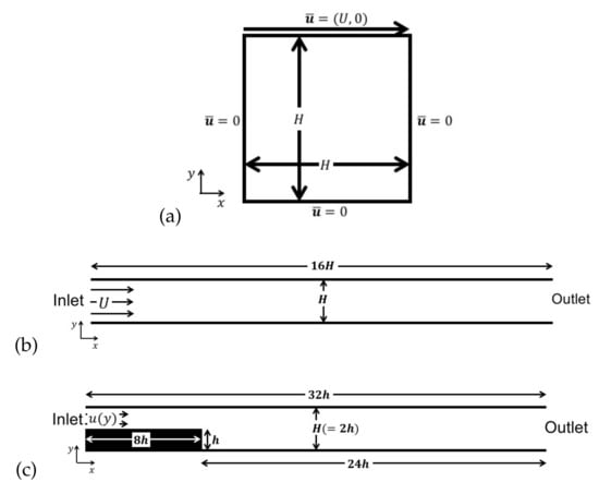
Figure 1.
The schematic model and coordinates systems: (a) flow in a lid-driven cavity, (b) flow in a channel, and (c) flow in a backward facing step.
7.1. Grid Sensitivity Test and Code Validation with Lid-Driven Cavity Flow
A square lid-driven cavity flow was considered to test the MPL model using the SRT lattice Boltzmann (LB) simulation for and 500 where and H indicate the maximum lid velocity and the height of the cavity, respectively. At the top wall of the cavity, a moving boundary condition was applied as , where and for the rest of the walls, a well known bounce-back condition was applied (for no slip walls). Before going to the code validation, firstly a grid-sensitivity test (GST) has been done in terms of the horizontal u velocity components for the maximum Reynolds number , with three different grid orientations; case 1: , case 2: , and Case 3: . The GIT results are illustrated in Figure 2a–c for the power-law indexes , 1, and , respectively. From these figures, it is clearly evident that the flow is grid independent. For , a lattice size of is considered in the present simulation and the obtained numerical results are depicted in Figure 3 for , and .
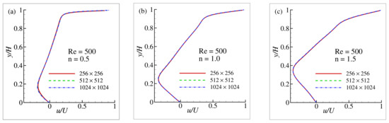
Figure 2.
Grid sensitivity test interms of the horizontal velocity profiles, , for the lid driven cavity (a) , (b) and (c) at .
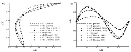
Figure 3.
Velocity profiles for the lid driven cavity (a) at and (b) at while .
In Figure 3a,b, the results obtained from the modified power-law (MPL) are compared with the available results of from the traditional power-law (PL) model for by Chai et al. [29], Neoftou [3], Bell and Surana [2], and Ghia et al. [64]. Results show an excellent agreement with the available results published before. In Figure 4a,b another comparison is shown in terms of the velocity distribution for with the Newtonian and non-Newtonian fluids. For , a lattice size of has been used for the simulation and the results exhibit very good agreement with the results of Neoftou [3].
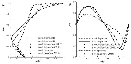
Figure 4.
Velocity profiles for the lid driven cavity (a) at and (b) at while .
Figure 5a–c and Figure 6a–c show the flow feature in terms of the streamlines for and 500, respectively. Figures show the results for the case of shear-thinning (), Newtonian (), and shear-thickening () fluids. It is apparent from the results that the core of the primary vortex has appeared near the driven lid. Besides the primary vortex, a secondary and tertiary vortex has emerged in the right and left bottom corners of the cavity with increasing the values of power-law index n. That happened because increasing the values of n led to increased viscosity inside the fluid, leading to the emergence of the corner vortex. It is also apparent that for larger , the size of the corner vortex increases.
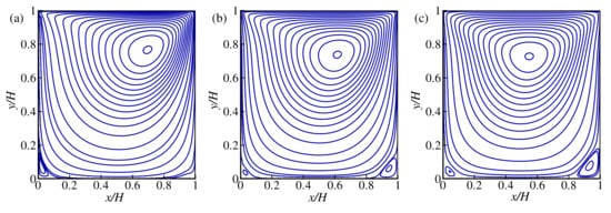
Figure 5.
Streamlines for the lid driven cavity flow: (a) , (b) (Newtonian), and (c) while .
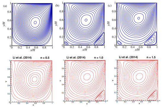
Figure 6.
Qualitative comparison of the the streamlines with the results of Li et al. [32] for the lid driven cavity flow: (a) (shear-thinning), (b) (Newtonian), and (c) (shear-thickening) while .
In Figure 6, there is a quantitative comparison in terms of the streamlines for the different power-law indexes, which means direct comparison with the published results by our numerical data. Qualitative comparison implies a comparison of two figures keeping side-by-side, and by inspection; it can be decided whether they look similar or not. A wualitative comparison of the streamlines with the results of Li et al. [32] for the lid-driven cavity flow was done while , and it shows that the agreement is good indeed. To support this qualitative comparison, again, a quantitative comparison is made by calculating the center of the primary vortex shown in the Table 2 and found excellent agreement with the available published results in the literature.
Table 2.
Comparison of the center of the primary vortex for the different power-law indexes n while .
7.2. Validation with Channel Flow
Here, we consider a simple 2D channel whose width is H, and the length is . In this case, a lattice size of is considered for the simulation study. At the top and bottom walls, the bounce-back condition is used, and at the left wall, an inflow boundary condition is applied with uniform velocity U. At the outlet (right wall), a zero gradient condition is employed. The available analytical solution for the power-law fluid regarding channel flow is given by
where U is the average velocity, the numerical result in terms of the stream-wise velocity obtained from LBM is compared with the analytical results obtained by Equation (24) for the power-law non-Newtonian fluids. Figure 7a–e show the axial velocity distributions for the different power-law index such as and respectively, while . The comparison in the figure shows that the numerical results establish an excellent agreement with the analytical results.
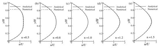
Figure 7.
Velocity profile for the channel flow at (a) , (b) , (c) , (d) , and (e) .
7.3. Flow in a Backward-Facing Step
There are no results available for the non-Newtonian power-law fluids in a backward-facing step while , so it is not possible to show a direct comparison for the code validation. Instead of the backward-facing step, for the power-law fluids, , a qualitative comparison is shown in terms of the streamlines with the results of power-law non-Newtonian fluids flow in a sudden expansion channel obtained by Ilio et al. [65] and depicted in Figure 8. Here the boundary conditions, the aspect ratio of the inlet and channel height (, where H is the channel height and d is the length of the inlet), and the length of the upstream and downstream regions are kept as same as Ilio et al. [65]. Based on Ilio et al. [65] study, the lattice size is chosen for this comparison. From these figures, it can be concluded that the comparison showed a good agreement.
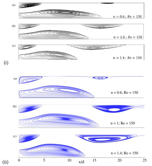
Figure 8.
Streamlines for the power-law non-Newtonian fluids flow in a sudden expansion channel with aspect ratio (): (i) BGK-LBM results of Ilio et al. [65] and (ii) present MRT-LBM for (a) , (b) and (c) .
Newtonian flow’s well-known benchmark problem through a backward-facing step has been considered for the non-Newtonian power-law fluids. In this study, the ratio between the channel hight and facing step height is chosen by . The facing step’s length is , and the length of the downstream region is 24 h. At the inlet of the backward facing-step, the parabolic velocity profile is used as inflow condition. Before going to the final simulation a grid-sensitivity test (GST) has been done using the three different lattice sizes ():case1 , case2 and case3 for the maximum while shear-thinning (), Newtonian () and shear-thickening (). For the shear-thinning fluid (), the flow is transitional, and it is not possible to get the instantaneous steady-state results. For this shear-thinning case, the time-mean results are calculated and eventually found steady-state results. Five million iterations have been taken for the shear-thinning fluid () flow simulations, and the last one million data samples are considered for calculating the time-mean results. From this GST, the numerical results are presented in terms of the primary recirculation zone () immediately after the step, and they are shown in Table 3. The lattice size for this simulation is considered by . The simulations have been done for different Reynolds number, , and 400 and for different power-law index such as (shear-thinning fluids), (Newtonian fluids), and (shear-thickening fluids).
Table 3.
Grid sensitivity test for the flow in a backward-facing step in terms of the length of reattachment point of the primary recirculation zone at the bottom wall for the different power-law index n while .
In backward-facing step flow, the flow separations and flow-reattachment are common phenomena to investigate. The reattachment point in the recirculation zones after the facing step appear for each power-law fluids n that are shown in Table 4. In the case of Newtonian fluid (), a comparison is made with the results of Erturk [48] (see in parenthesis) and found a good agreement. It should be mentioned that similar boundary conditions of Erturk [48] have been used in the present simulation. For shear-thinning fluids, the length of the recirculation zone increases for decreasing the values of n. On the other hand, the recirculation zone’s length decreases for increasing n in shear-thickening fluids. It is obvious because in shear-thinning fluids, decreasing the power-law index (n) leads to reduce fluid viscosity and accelerates the fluid velocity. As a result, the recirculation zone is getting larger after the backward-facing step. The opposite phenomenon is observed for shear-thickening fluid while increasing the value of n. The depiction of the steady-state recirculation zones for (left) and 200 (right) with different power-law index such as , and are shown in the Figure 9. These results showed a good agreement with the length of the reconciliation zone. The effect of power-law index on the flow of backward-facing step for and 400 is shown in Figure 10 and Figure 11. Here the flow becomes laminar-to-transition in shear-thinning fluids, and the large vortex splits into several vortices for both the values of and 400. For these Reynolds number and shear-thinning cases, it becomes difficult to measure the steady-state recirculation zone. For the Newtonian fluid, the length of the primary recirculation zone’s reattachment point expands with increasing the value of ; however, several recirculation zones are observed in the shear-thinning fluid in the flow domain.
Table 4.
Length of reattachment point of the primary recirculation zone at the bottom wall for the different power-law indexes n and for different Reynolds numbers .
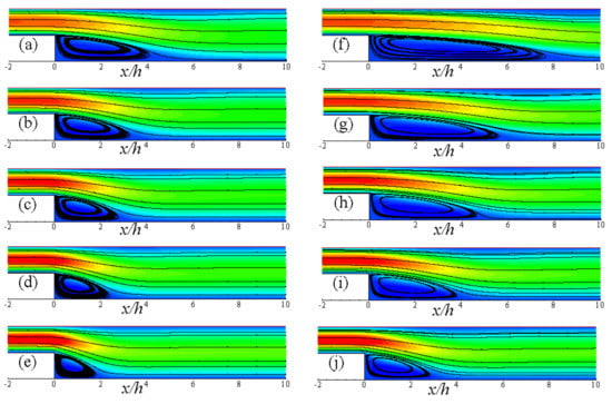
Figure 9.
Streamlines for different power-law indexes: (a) , (b) , (c) , (d) , (e) while (left) and (f) , (g) , (h) , (i) , (j) while (right).
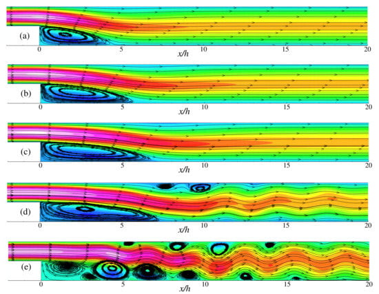
Figure 10.
Streamlines for different power-law indexes: (a) , (b) , (c) , (d) , (e) while .
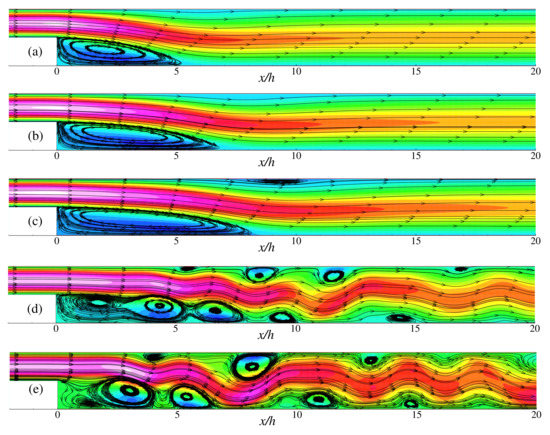
Figure 11.
Streamlines for different power-law indexes: (a) , (b) , (c) , (d) , (e) while .
Figure 12 and Figure 13 illustrate the axial velocity profiles at the different location of for and while and 200, respectively. For both the Reynolds numbers, the velocity profile’s variation is prominent for the shear-thinning fluids due to the large recirculation zones. The velocity gets a negative magnitude near the lower wall within the recirculation zones, as one can observe in different frames corresponding to the channel’s different positions. The negative velocity intensity is higher in the shear-thinning fluids () and lower for the shear-thickening fluids (). Near the upper wall, the velocity distribution increases for decreasing the values of the power-law index n; i.e., fluid velocity becomes augmented for the shear-thinning case . For higher Reynolds number , the shear-thinning effect on the augmentation of velocity grows up to the length of .
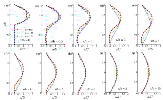
Figure 12.
Velocity distribution at the different axial locations of the downstream region while and n (=0.5, 1.0, 1.5).
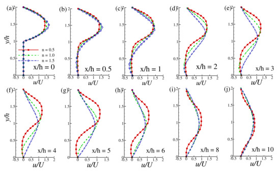
Figure 13.
Velocity distribution at the different axial locations of the downstream region while and n (=0.5, 1.0, 1.5).
The effect of the power-law index n (=0.5, 0.8, 1.0, 1.2, and 1.5) on the wall shear stress is investigated in terms of the local skin-friction coefficient as displayed in Figure 14a,b and Figure 15a,b for different Reynolds numbers, , and 400. Here is considered for the present numerical simulation. The effect of the power-law index is visible on the wall shear stress. It is known that increasing the values of n leads to increased fluid viscosity and, consequently, enhances the wall shear stress intensity. The phenomena are quite apparent in Figure 14. Results show that increasing the power-law index leads to a decrease in the re-circulation zone where due to the negative velocity near the wall. Within the re-circulation zone, gets stronger in the negative direction with increasing the power-law index . After the flow gets reattached to the wall, becomes stronger in the positive direction for shear-thickening fluids than the Newtonian and the shear-thinning fluids . For , the intensity of the wall shear stress increases in magnitude in the re-circulation zone, while decreases in the next reattachment region for all types of fluids. Further increasing the Reynolds number to and , as shown in Figure 15, the wall shear stress show periodic nature for shear-thinning fluids as there exist several re-circulation zones and reattachment region along the bottom wall for these fluids. The feature of shear-thickening fluids showing higher wall shear stress in magnitude still present for . For , the amplitude of the periodic nature of for shear-thinning fluids gets stronger. In this case, becomes higher for shear-thinning fluids than the shear-thickening fluids at some regions on the wall shear stress. We assume that at , shear-thinning fluids do not behave like laminar rather transitional. It is found that with increasing the values of , the shear-thickening fluids exhibit less intensity of wall shear stress, but the shear-thinning fluids tend to show the periodic nature of wall shear stress with increasing amplitude.
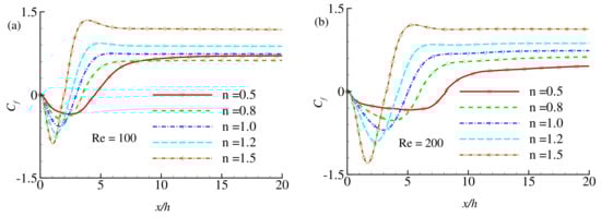
Figure 14.
Skin-friction coefficient, at the lower wall for the different values of power-law index n at (a) and (b) .
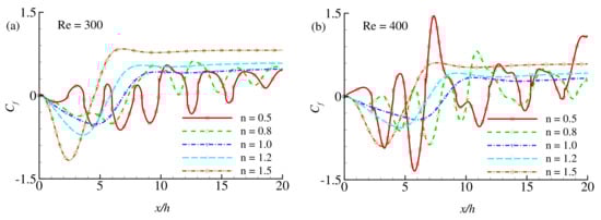
Figure 15.
Skin-friction coefficient, at the lower wall for the different values of power-law index n at (a) and (b) .
It is possible to find numerous studies in the literature considering the flow in a backward-facing step. However, still, there is a lack of tabulated data in hand. In this study, the results are presented in tabular form in order to facilitate the comparison. Table 5 and Table 6 present the tabular values of u-velocity profiles for and 400, respectively, and for different values of power-law index across the channel at different location , , and .
Table 5.
Tabulated u-velocity profiles for .
Table 6.
Tabulated u-velocity profiles for .
8. Conclusions
In this paper, a modified power-law viscosity model for the generalized Newtonian fluid is used for the lattice Boltzmann method and validated by comparing with numerical and analytical results of well-known benchmark problems and then applied for fluid flow in a backward-facing step. In this MPL model, one distinct time unit parameter for the LBM has been identified that governs the non-Newtonian fluid flows. In the traditional power-law model for a very low shear rate, the effective viscosity is very large or infinity. For the substantial shear rate, the viscosity is very low or vanishes in shear-thinning fluids, causing the unstable LBM simulation. For the shear-thickening fluids, the opposite phenomena appear. This MPL model removes the deficiencies of the traditional PL model. Hence, there are no singularities in MPL and there is no chance to be a viscosity-less fluid (solid) in the simulation.
The MRT-LBM code and the proposed modified power-law viscosity model have been validated with the benchmark results for the different power-law index, n. Finally, the investigation has been done for the power-law fluid flows in a backward-facing step for the different Reynolds number. The length of the re-attachment point decreases for increasing the power-law index from the shear-thinning () to shear-thickening fluids () fluids. In the shear-thinning case , the flow is transitional while , and the large vortex breaks down into small eddies. The flow is always laminar for the shear-thickening fluids due to the higher viscosity of the fluid. On the other hand, for increasing the Reynolds number, , the re-attachment point’s length increases while the flow is laminar. The numerical results of the flow in backward-facing step for the power-law fluids may be used as benchmark results for low Reynolds numbers. In the near future, the investigation would be done for .
Author Contributions
First author: M.M.M. has modeled the problem, developed the CUDA C code, visualize the figures and written the manuscript; Second author: P.N. has extended the some parts of the introduction and edited the whole manuscript; Third author: S.T. has constructed the tables and edited the results and discussion part; Fourth author: A.K. has helped to develop the CUDA C code and edited the manuscript. All authors have read and agreed to the published version of the manuscript
Funding
“This work is funded by Faculty Research Grant (CTRG grant No.: NSU-RP-18-067 and CTRG19/SEPS/15), North South University, Dhaka, Bangladesh” and “The APC was funded by MDPI as author (MMM) voucher discount.”
Acknowledgments
The first author M. M. Molla would like to thank the NVIDIA Corporation, USA, for granting the TESLA k40 GPU.
Conflicts of Interest
We are declaring that there is no conflict of interest for publishing this article.
Appendix A
Here the derivation of for the modified power-law is given as follows:
where which is free from the power-law index and gives a constant reference kinematic viscosity for a fixed and lattice size. Here . For the modified power-law model the definition of is not generalized. (“PL= power-law” amd “MPL= modifiled power-law”).
References
- Chhabra, R.P.; Richardson, J.F. Non-Newtonian Flow in the Process Industries: Fundamentals and Engineering Applications; Butterworth-Heinemann: Oxford, UK, 1999. [Google Scholar]
- Bell, B.C.; Surana, K.S. p-version least squares finite element formulation for two-dimensional, incompressible, non-Newtonian isothermal and non-isothermal fluid flow. Int. J. Numer. Methods Fluids 1994, 18, 127–162. [Google Scholar] [CrossRef]
- Neofytou, P. A 3rd order upwind finite volume method for generalised Newtonian fluid flows. Adv. Eng. Softw. 2005, 36, 664–680. [Google Scholar] [CrossRef]
- Rafiee, A. Modelling of generalized Newtonian lid-driven cavity flow using an SPH method. ANZIAM J. 2008, 49, 411–422. [Google Scholar] [CrossRef]
- Syrjälä, S. Finite-element analysis of fully developed laminar flow of power-law non-Newtonian fluid in a rectangular duct. Int. Commun. Heat Mass Transf. 1995, 22, 549–557. [Google Scholar] [CrossRef]
- Bose, A.; Carey, G. Least-squares pr finite element methods for incompressible non-Newtonian flows. Comput. Methods Appl. Mech. Eng. 1999, 180, 431–458. [Google Scholar] [CrossRef]
- Benzi, R.; Succi, S.; Vergassola, M. The lattice Boltzmann equation: Theory and applications. Phys. Rep. 1992, 222, 145–197. [Google Scholar] [CrossRef]
- Succi, S. The Lattice Boltzmann Equation: For Fluid Dynamics and Beyond; Oxford University Press: Oxford, UK, 2001. [Google Scholar]
- Wolf-Gladrow, D.A. Lattice-Gas Cellular Automata and Lattice Boltzmann Models: An Introduction; Springer: Berlin/Heidelberg, Germany, 2004. [Google Scholar]
- Higuera, F.; Succi, S.; Benzi, R. Lattice gas dynamics with enhanced collisions. EPL Europhys. Lett. 1989, 9, 345. [Google Scholar] [CrossRef]
- Succi, S.; Foti, E.; Higuera, F. Three-dimensional flows in complex geometries with the lattice Boltzmann method. EPL Europhys. Lett. 1989, 10, 433. [Google Scholar] [CrossRef]
- Lavallée, P.; Boon, J.P.; Noullez, A. Boundaries in lattice gas flows. Phys. Nonlinear Phenom. 1991, 47, 233–240. [Google Scholar] [CrossRef]
- Ziegler, D.P. Boundary conditions for lattice Boltzmann simulations. J. Stat. Phys. 1993, 71, 1171–1177. [Google Scholar] [CrossRef]
- D’Humieres, D. Generalized lattice Boltzmann Equations, Rarefied Gas Dynamics: Theory and Simulations. Prog. Astronaut. Aeronaut. 1992, 159, 450–458. [Google Scholar]
- Lallemand, P.; Luo, L.S. Theory of the lattice Boltzmann method: Dispersion, dissipation, isotropy, Galilean invariance, and stability. Phys. Rev. E 2000, 61, 6546. [Google Scholar] [CrossRef] [PubMed]
- D’Humieres, D. Multiple–relaxation–time lattice Boltzmann models in three dimensions. Philos. Trans. R. Soc. Lond. Ser. A Math. Phys. Eng. Sci. 2002, 360, 437–451. [Google Scholar]
- Du, R.; Shi, B.; Chen, X. Multi-relaxation-time lattice Boltzmann model for incompressible flow. Phys. Lett. A 2006, 359, 564–572. [Google Scholar] [CrossRef]
- Liu, Y.; So, R.; Cui, Z. Bluff body flow simulation using lattice Boltzmann equation with multiple relaxation time. Comput. Fluids 2006, 35, 951–956. [Google Scholar] [CrossRef]
- Mezrhab, A.; Moussaoui, M.A.; Jami, M.; Naji, H.; Bouzidi, M. Double MRT thermal lattice Boltzmann method for simulating convective flows. Phys. Lett. A 2010, 374, 3499–3507. [Google Scholar] [CrossRef]
- Li, Z.; Yang, M.; Zhang, Y. Lattice Boltzmann method simulation of 3-D natural convection with double MRT model. Int. J. Heat Mass Transf. 2016, 94, 222–238. [Google Scholar] [CrossRef]
- Liu, Q.; Feng, X.B.; He, Y.L.; Lu, C.W.; Gu, Q.H. Three-dimensional multiple-relaxation-time lattice Boltzmann models for single-phase and solid-liquid phase-change heat transfer in porous media at the REV scale. Appl. Therm. Eng. 2019, 152, 319–337. [Google Scholar] [CrossRef]
- Mai, H.C.; Lin, K.H.; Yang, C.H.; Lin, C.A. A thermal lattice Boltzmann model for flows with viscous heat dissipation. Comput. Model Eng. Sci. 2010, 61, 45–62. [Google Scholar]
- Bao, Y.B.; Meskas, J. Lattice Boltzmann Method for Fluid Simulations; Department of Mathematics, Courant Institute of Mathematical Sciences, New York University: New York, NY, USA, 2011. [Google Scholar]
- Kuznik, F.; Obrecht, C.; Rusaouen, G.; Roux, J.J. LBM based flow simulation using GPU computing processor. Comput. Math. Appl. 2010, 59, 2380–2392. [Google Scholar] [CrossRef]
- Tölke, J. Implementation of a lattice Boltzmann kernel using the Compute Unified Device Architecture developed by nVIDIA. Comput. Vis. Sci. 2010, 13, 29–39. [Google Scholar] [CrossRef]
- Ren, Q.; Chan, C.L. Numerical study of double-diffusive convection in a vertical cavity with Soret and Dufour effects by lattice Boltzmann method on GPU. Int. J. Heat Mass Transf. 2016, 93, 538–553. [Google Scholar] [CrossRef]
- Phillips, T.N.; Roberts, G.W. Lattice Boltzmann models for non-Newtonian flows. IMA J. Appl. Math. 2011, 76, 790–816. [Google Scholar] [CrossRef]
- Nejat, A.; Abdollahi, V.; Vahidkhah, K. Lattice Boltzmann simulation of non-Newtonian flows past confined cylinders. J. Non-Newton. Fluid Mech. 2011, 166, 689–697. [Google Scholar] [CrossRef]
- Chai, Z.; Shi, B.; Guo, Z.; Rong, F. Multiple-relaxation-time lattice Boltzmann model for generalized Newtonian fluid flows. J. Non-Newton. Fluid Mech. 2011, 166, 332–342. [Google Scholar] [CrossRef]
- Mendu, S.S.; Das, P.K. Flow of power-law fluids in a cavity driven by the motion of two facing lids- simulation by lattice Boltzmann method. J. Non-Newton. Fluid Mech. 2012, 175–176, 10–24. [Google Scholar] [CrossRef]
- Delouei, A.M.; Nazari, M.; Kayhani, M.H.; Succi, S. Non-Newtonian unconfined flow and heat transfer over a heated cylinder using the direct-forcing immersed boundary–thermal lattice Boltzmann method. Phys. Rev. E 2014, 89, 053312. [Google Scholar] [CrossRef]
- Li, Q.; Hong, N.; Shi, B.; Chai, Z. Simulation of power-law fluid flows in two-dimensional square cavity using multi-relaxation-time lattice boltzmann method. Commun. Comput. Phys. 2014, 15, 265–284. [Google Scholar] [CrossRef]
- Riesinger, C.; Bakhtiari, A.; Schreiber, M.; Neumann, P.; Bungartz, H.J. A holistic scalable implementation approach of the lattice Boltzmann method for CPU/GPU heterogeneous clusters. Computation 2017, 5, 48. [Google Scholar] [CrossRef]
- Geier, M.; Schoenherr, M. Esoteric twist: An efficient in-place streaming algorithmus for the lattice Boltzmann method on massively parallel hardware. Computation 2017, 5, 19. [Google Scholar] [CrossRef]
- Franco, E.E.; Barrera, H.M.; Laín, S. 2D lid-driven cavity flow simulation using GPU-CUDA with a high-order finite difference scheme. J. Braz. Soc. Mech. Sci. Eng. 2015, 37, 1329–1338. [Google Scholar] [CrossRef]
- Molla, M.M.; Haque, M.J.; Khan, A.; Saha, S.C. GPU Accelerated Multiple-Relaxation-Time Lattice Boltzmann Simulation of Convective Flows in a Porous Media. Front. Mech. Eng. 2018, 4, 1–17. [Google Scholar] [CrossRef]
- Jin, K.; Vanka, S.; Agarwal, R.; Thomas, B. GPU accelerated simulations of three-dimensional flow of power-law fluids in a driven cube. Int. J. Comput. Fluid Dyn. 2017, 31, 36–56. [Google Scholar] [CrossRef]
- Rahim, K.Z.; Ahmed, J.; Nag, P.; Molla, M.M. Lattice Boltzmann simulation of natural convection and heat transfer from multiple heated blocks. Heat Transf. 2020, 49, 1877–1894. [Google Scholar] [CrossRef]
- Bird, R.B.; Armstrong, R.C.; Hassager, O. Dynamics of Polymeric Liquids, Vol. 1: Fluid Mechanics; John Wiley and Sons Inc.: New York, NY, USA, 1987. [Google Scholar]
- Chhabra, R.P.; Richardson, J.F. Non-Newtonian Flow and Applied Rheology: Engineering Applications, 2nd ed.; Butterworth Heinemann: Oxford, UK, 2008. [Google Scholar]
- Bird, R.B.; Stewart, W.E.; Lightfoot, W.E. Transport Phenomena; JohnWiley & Sons: New York, NY, USA, 2002. [Google Scholar]
- Yao, L.S.; Molla, M.M. Forced convection of non-Newtonian fluids on a heated flat plate. Int. J. Heat Mass Transf. 2008, 51, 5154–5159. [Google Scholar] [CrossRef]
- Boger, D.V. Demonstration of upper and lower Newtonian fluid behaviour in a pseudoplastic fluid. Nature 1977, 265, 126–128. [Google Scholar] [CrossRef]
- Molla, M.M.; Yao, L.S. The flow of non-newtonian fluids on a flat plate with a uniform heat flux. J. Heat Transf. 2009, 131, 011702. [Google Scholar] [CrossRef]
- Chen, L.; Asai, K.; Nonomura, T.; Xi, G.; Liu, T. A review of Backward-Facing Step (BFS) flow mechanisms, heat transfer and control. Therm. Sci. Eng. Prog. 2018, 6, 94–216. [Google Scholar] [CrossRef]
- Lee, T.; Mateescu, D. Experimental and numerical investigation of 2-D backward-facing step flow. J. Fluids Struct. 1998, 12, 703–716. [Google Scholar] [CrossRef]
- Armaly, B.F.; Durst, F.; Pereira, J.; Schönung, B. Experimental and theoretical investigation of backward-facing step flow. J. Fluid Mech. 1983, 127, 473–496. [Google Scholar] [CrossRef]
- Erturk, E. Numerical solutions of 2-D steady incompressible flow over a backward-facing step, Part I: High Reynolds number solutions. Comput. Fluids 2008, 37, 633–655. [Google Scholar] [CrossRef]
- Xiong, W.; Zhang, J. A two-dimensional lattice Boltzmann model for uniform channel flows. Comput. Math. Appl. 2011, 61, 3453–3460. [Google Scholar] [CrossRef][Green Version]
- Zhou, J.G.; Liu, H.; Shafiai, S.; Peng, Y.; Burrows, R. Lattice boltzmann method for open-channel flows. Proc. Inst. Civ. Eng.-Eng. Comput. Mech. 2010, 163, 243–249. [Google Scholar] [CrossRef]
- Wu, J.S.; Shao, Y.L. Simulation of lid-driven cavity flows by parallel lattice Boltzmann method using multi-relaxation-time scheme. Int J. Numer. Methods Fluids 2004, 46, 921–937. [Google Scholar] [CrossRef]
- Velivelli, A.C.; Bryden, K.M. Domain decomposition based coupling between the lattice Boltzmann method and traditional CFD methods—Part II: Numerical solution to the backward facing step flow. Adv. Eng. Softw. Thomson Reuters 2015, 82, 65–74. [Google Scholar] [CrossRef]
- Ameur, H.; Menni, Y. Non-Newtonian fluid flows through backward-facing steps. SN Appl. Sci. 2019, 1, 1717. [Google Scholar] [CrossRef]
- Shupti, S.P.; Molla, M.M.; Mia, M. Pulsatile non-Newtonian fluid flows in a model aneurysm with oscillating wall. Front. Mech. Eng. 2017, 3, 12. [Google Scholar] [CrossRef]
- Siddiki, M.N.A.A.; Molla, M.M.; Thohura, S.; Saha, S.C. Lattice Boltzmann simulation of Non-Newtonian power-law fluid flows in a bifurcated channel. In AIP Conference Proceedings; AIP Publishing LLC: New York, NY, USA, 2018; Volume 1980, p. 040023. [Google Scholar]
- Thohura, S.; Molla, M.M.; Sarker, M. Natural convection of non-Newtonian shear-thinning fluid flow inside a skewed cavity. In AIP Conference Proceedings; AIP Publishing LLC: New York, NY, USA, 2019; Volume 2121, p. 030014. [Google Scholar]
- Thohura, S.; Molla, M.M.; Sarker, M.M.A. Numerical simulation of non-Newtonian power-law fluid flow in a lid-driven skewed cavity. Int. J. Appl. Comput. Math. 2019, 5, 14. [Google Scholar] [CrossRef]
- Thohura, S.; Molla, M.M.; Sarker, M. Bingham fluid flow simulation in a lid-driven skewed cavity using the finite-volume method. Int. J. Comput. Math. 2020, 97, 1212–1233. [Google Scholar] [CrossRef]
- Chai, Z.; Shi, B.; Guo, Z. A multiple-relaxation-time lattice Boltzmann model for general nonlinear anisotropic convection–diffusion equations. J. Sci. Comput. 2016, 69, 355–390. [Google Scholar] [CrossRef]
- Molla, M.M.; Yao, L.S. Non-Newtonian natural convection along a vertical heated wavy surface using a modified Power-Law Viscosity Model. J. Heat Transf. 2009, 131, 012501. [Google Scholar] [CrossRef]
- Zou, Q.; He, X. On pressure and velocity boundary conditions for the lattice Boltzmann BGK model. Phys. Fluids 1997, 9, 1591–1598. [Google Scholar] [CrossRef]
- Nvidia, C. C Programming Guide Version 4.0; Nvidia Corporation: Clara, CA, USA, 2011. [Google Scholar]
- Jahidul Haque, M.; Mamun Molla, M.; Amirul Islam Khan, M.; Ahsan, K. Graphics process unit accelerated lattice Boltzmann simulation of indoor air flow: Effects of sub-grid scale model in large-eddy simulation. Proc. Inst. Mech. Eng. Part C J. Mech. Eng. Sci. 2020, 234, 4024–4040. [Google Scholar] [CrossRef]
- Ghia, U.G.; Ghia, K.N.; Shin, C.T. High-Re solutions for incompressible flow using the Navier-Stokes equations and a multigrid method. J. Comp. Phys. 1982, 48, 387–411. [Google Scholar] [CrossRef]
- Ilio, G.D.; Chiappini, D.; Bella, G. A comparison of numerical methods for non-Newtonian fluid flows in a sudden expansion. Int. J. Mod. Phys. C 2016, 27, 1650139. [Google Scholar] [CrossRef]


© 2020 by the authors. Licensee MDPI, Basel, Switzerland. This article is an open access article distributed under the terms and conditions of the Creative Commons Attribution (CC BY) license (http://creativecommons.org/licenses/by/4.0/).