
Online Adaptive Local-Global Model Reduction for Flows in Heterogeneous Porous Media


Abstract
:
1. Introduction
2. Preliminaries
2.1. Proper Orthogonal Decomposition
2.2. Discrete Empirical Interpolation Method (DEIM)
2.3. Local Model Order Reduction via GMsFEM
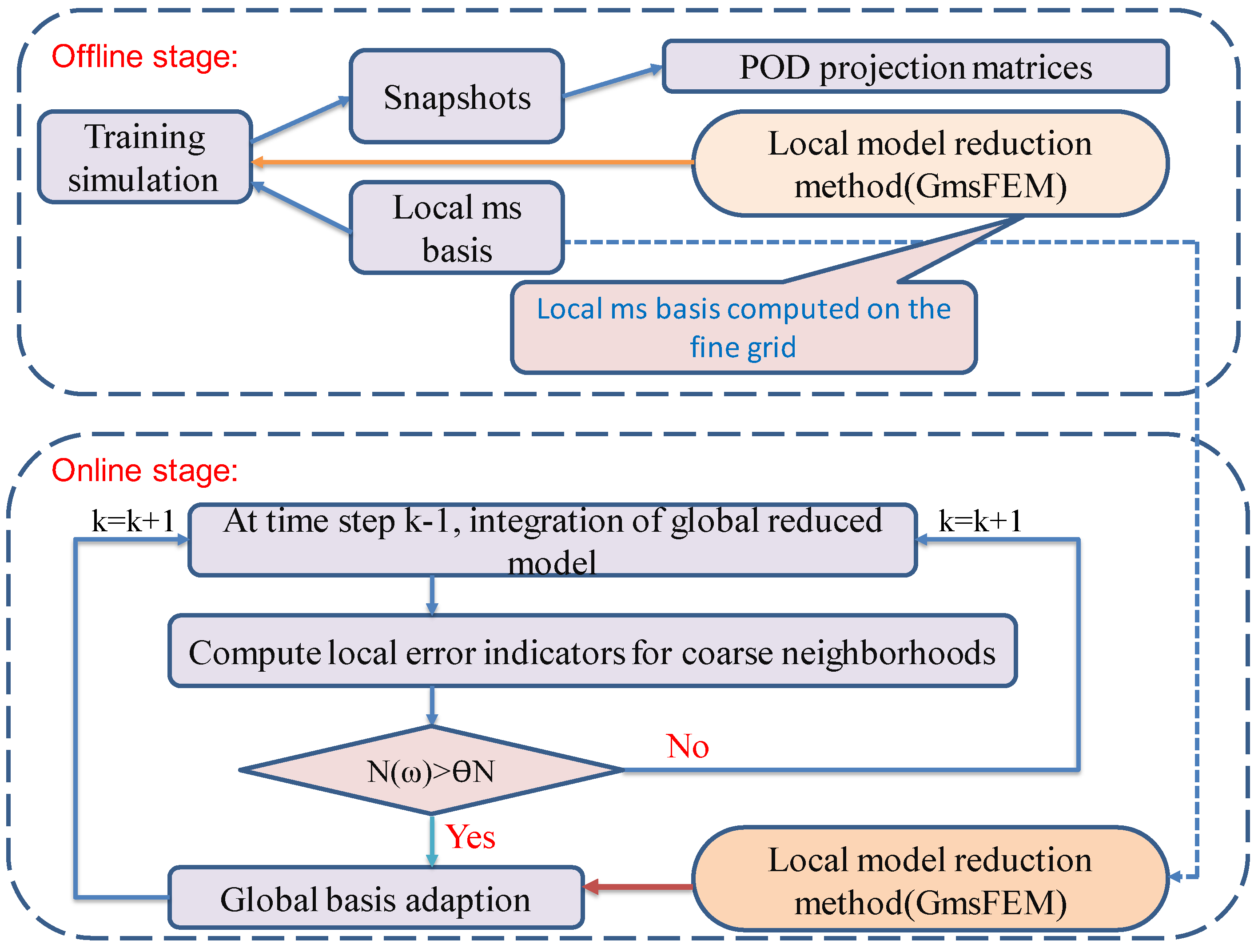
3. Online Adaptive POD-DEIM Model Reduction
3.1. Online Adaptive Local-Global Proper Orthogonal Decomposition
| Algorithm 1 Adaptive Local-Global POD Model Order Reduction Method | |
| OFFLINE STAGE: | |
| 1: | Construction of snapshots for states, local off-line space (consists of local ms basis) by GMsFEM |
| 2: | Construction of POD subspaces (POD projection matrices) |
| ONLINE STAGE : for step k adaption | |
| 3: | INPUT : Global POD basis matrix , local off-line space |
| 4: | Solve the reduced system: (Global reduced-order model) |
| 5: | Compute local error indicators, and decide if adaption is needed. If yes, go to 6. Otherwise, go to next time step |
| 6: | Solve the global residual problem for by adaptive local method with initial local off-line space |
| 7: | Update the POD subspace by Adaptive-POD-1 or Adaptive-POD-2 |
| 8: | OUTPUT : Global POD basis matrix , local offline space |
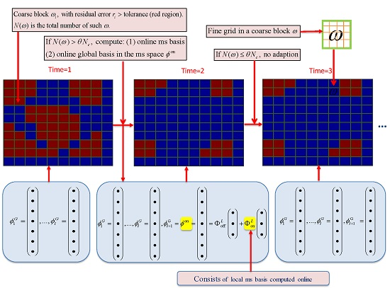
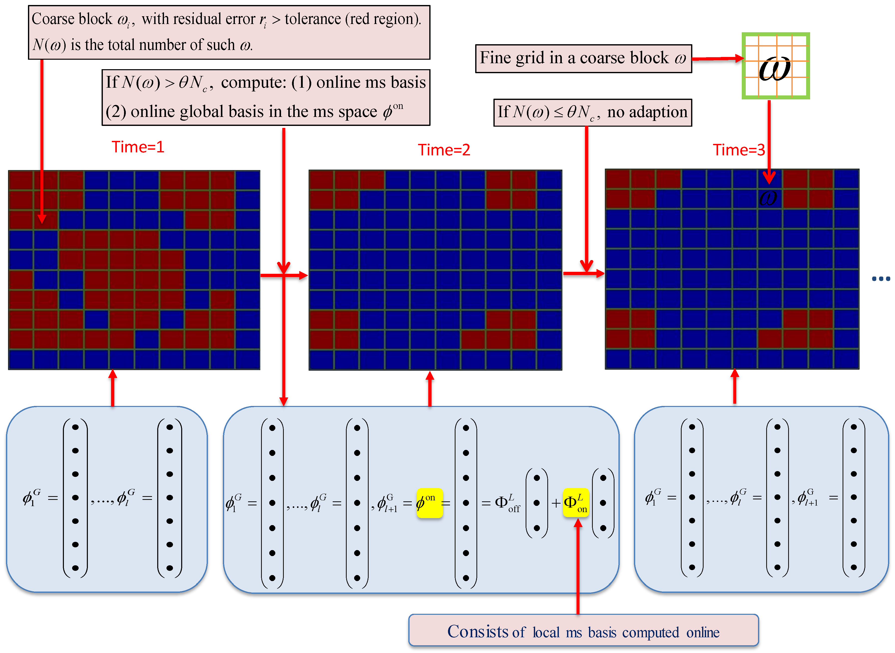
- For coarse blocks , compute their corresponding norm of the residual, and denote as .
- Count the total number of coarse blocks with a certain error tolerance. Here a large error means the current POD modes cannot give a good representation of the features in that coarse block.
- If , then adaption is needed, θ is a fraction of the total number of coarse blocks.
3.2. Online Adaptive DEIM
| Algorithm 2 Online Adaptive DEIM [25] |
|
4. Applications
4.1. Single-Phase Flow
4.2. Two-Phase Flow
4.2.1. An Incompressible Two-Phase Flow Model
4.2.2. Numerical Example
5. Conclusion
Acknowledgments
Author Contributions
Conflicts of Interest
References
- Lumley, J. Atmospheric turbulence and radio wave propagation. J. Comput. Chem. 1967, 23, 1236–1243. [Google Scholar]
- Gugercin, S.; Antoulas, A. A survey of model reduction by balanced truncation and some new results. Int. J. Control 2004, 77, 748–766. [Google Scholar] [CrossRef]
- Rewienski, M.; White, J. A trajectory piecewise-linear approach to model order reduction and fast simulation of nonlinear circuits and micromachined devices. IEEE Trans. Comput.-Aided Des. Intergrated Circ. Syst. 2003, 22, 155–170. [Google Scholar] [CrossRef]
- Hall, K.C.; Thomas, J.P.; Dowell, E.H. Proper orthogonal decomposition technique for transonic unsteady aerodynamic flows. AIAA J. 2000, 38, 1853–1862. [Google Scholar] [CrossRef]
- Kunisch, K.; Volkwein, S. Control of the burgers equation by a reduced-order approach using proper orthogonal decomposition. J. Optim. Theory Appl. 1999, 102, 345–371. [Google Scholar] [CrossRef]
- Rowley, C.W.; Colonius, T.; Murray, R.M. Model reduction for compressible flows using POD and Galerkin projection. Phys. D 2004, 189, 115–129. [Google Scholar] [CrossRef]
- Bui-Thanh, T.; Damodaran, M.; Willcox, K. Aerodynamic data reconstruction and inverse design using proper orthogonal decomposition. AIAA J. 2004, 42, 1505–1516. [Google Scholar] [CrossRef]
- Meyer, M.; Matthies, H. Efficient model reduction in non-linear dynamics using the karhunen-loève expansion and dual-weighted-residual methods. Comput. Mech. 2003, 31, 179–191. [Google Scholar] [CrossRef]
- Heijn, T.; Markovinovic, R.; Jansen, J. Generation of low-order reservoir models using system-theoretical concepts. SPE J. 2004, 9, 202–218. [Google Scholar] [CrossRef]
- Cardoso, M.; Durlofsky, L.; Sarma, P. Development and application of reduced-order modeling procedures for subsurface flow simulation. Int. J. Numer. Method. Eng. 2009, 77, 1322–1350. [Google Scholar] [CrossRef]
- Ghasemi, M.; Yang, Y.; Gildin, E.; Efendiev, Y.; Calo, V. Fast multiscale reservoir simulations using POD-DEIM model reduction. In Proceedings of the SPE Reservoir Simulation Symposium, Society of Petroleum Engineers, Houston, TX, USA, 23–25 February 2015. [CrossRef]
- Haasdonk, B.; Ohlberger, M. Adaptive basis enrichment for the reduced basis method applied to finite volume schemes. In Finite Volumes for Complex Applications V; Wiley-ISTE: Hoboken, NJ, USA; London, UK, 2008; pp. 471–479. [Google Scholar]
- Peherstorfer, B.; Butnaru, D.; Willcox, K.; Bungartz, H.-J. Localized discrete empirical interpolation method. SIAM J. Sci. Comput. 2014, 36, A168–A192. [Google Scholar] [CrossRef]
- Maday, Y.; Stamm, B. Locally adaptive greedy approximations for anisotropic parameter reduced basis spaces. SIAM J. Sci. Comput. 2013, 35, A2417–A2411. [Google Scholar] [CrossRef]
- Amsallem, D.; Farhat, C. An online method for interpolating linear parametric reduced-order models. SIAM J. Sci. Comput. 2011, 33, 2169–2198. [Google Scholar] [CrossRef]
- Chaturantabut, S.; Sorensen, D.C. Discrete empirical interpolation for nonlinear model reduction. SIAM J. Sci. Comput. 2010, 32, 2737–2764. [Google Scholar] [CrossRef]
- Efendiev, Y.; Galvis, J.; Hou, T.Y. Generalized multiscale finite element methods (gmsfem). J. Comput. Phys. 2013, 251, 116–135. [Google Scholar] [CrossRef]
- Efendiev, Y.; Hou, T.Y. Multiscale Finite Element Methods: Theory And Applications; Springer Science & Business Media: New York, NY, USA, 2009; Volume 4. [Google Scholar]
- Chung, E.; Efendiev, Y.; Hou, T.Y. Adaptive multiscale model reduction with generalized multiscale finite element methods. J. Comput. Phys. 2016. [Google Scholar] [CrossRef]
- Efendiev, Y.; Galvis, J.; Wu, X.-H. Multiscale finite element methods for high-contrast problems using local spectral basis functions. J. Comput. Phys. 2011, 230, 937–955. [Google Scholar] [CrossRef]
- Chung, E.T.; Efendiev, Y.; Li, G. An adaptive gmsfem for high-contrast flow problems. J. Comput. Phys. 2014, 273, 54–76. [Google Scholar] [CrossRef]
- Chung, E.T.; Efendiev, Y.; Leung, W.T. Residual-driven online generalized multiscale finite element methods. J. Comput. Phys. 2015, 302, 176–190. [Google Scholar] [CrossRef]
- Chung, E.T.; Leung, W.T.; Pollock, S. Goal-oriented adaptivity for gmsfem. J. Comput. Appl. Math. 2016, 296, 625–637. [Google Scholar] [CrossRef]
- Chan, H.Y.; Chung, E.T.; Efendiev, Y. Adaptive mixed gmsfem for flows in heterogeneous media. arXiv preprint 2015. [Google Scholar]
- Peherstorfer, B.; Willcox, K. Online adaptive model reduction for nonlinear systems via low-rank updates. SIAM J. Sci. Comput. 2015, 37, 2123–2150. [Google Scholar] [CrossRef]
- Alotaibi, M.; Calo, V.M.; Efendiev, Y.; Galvis, J.; Ghommem, M. Global–local nonlinear model reduction for flows in heterogeneous porous media. Comput. Method. Appl. Mech. Eng. 2015, 292, 122–137. [Google Scholar] [CrossRef]
- Efendiev, Y.; Galvis, J.; Gildin, E. Local–global multiscale model reduction for flows in high-contrast heterogeneous media. J. Comput. Phys. 2012, 231, 8100–8113. [Google Scholar] [CrossRef]
- Durlofsky, L.; Efendiev, Y.; Ginting, V. An adaptive local–global multiscale finite volume element method for two-phase flow simulations. Adv. Water Resour. 2007, 30, 576–588. [Google Scholar] [CrossRef]
- Presho, M.; Ye, S. Reduced-order multiscale modeling of nonlinear p-laplacian flows in high-contrast media. Comput. Geosci. 2015, 19, 921–932. [Google Scholar] [CrossRef]
- Vermeulen, P.; Heemink, A.; Stroet, C. Reduced models for linear groundwater flow models using empirical orthogonal functions. Adv. Water Resour. 2004, 27, 57–69. [Google Scholar] [CrossRef]
- Van Doren, J.; Markovinovic, R.; Jansen, J. Reduced-order optimal control of water flooding using proper orthogonal decomposition. Comput. Geosci. 2006, 10, 137–158. [Google Scholar] [CrossRef]
- Cardoso, M.; Durlofsky, L. Linearized reduced-order models for subsurface flow simulation. J. Comput. Phys. 2010, 229, 681–700. [Google Scholar] [CrossRef]
- Efendiev, Y.; Galivs, J.; Gildin, E. Local-global multiscale model reduction for flows in high-contrast heterogeneous media. J. Comput. Phys. 2012, 231, 8100–8113. [Google Scholar] [CrossRef]
- He, J.; Durlofsky, L.J. Constraint reduction procedures for reduced-order subsurface flow models based on POD-TPWL. Int. J. Numer. Meth. Eng. 2015. [Google Scholar] [CrossRef]
- Yang, Y.; Ghasemi, M.; Gildin, E.; Efendiev, Y.; Calo, V. Fast multi-scale reservoir simulations using POD-DEIM model reduction. In Proceedings of the SPE Reservoir Simulation Symposium, Houston, TX, USA, 23–25 February 2015. [CrossRef]
- Kunisch, K.; Volkwein, S. Galerkin proper orthogonal decomposition methods for a general equation in fluid dynamics. SIAM J. Numer. Anal. 2002, 40, 492–515. [Google Scholar] [CrossRef]
- Volkwein, S.; Hinze, M. Proper orthogonal decomposition surrogate models for nonlinear dynamical systems: Error estimates and suboptimal control. In Reduction of Large-Scale Systems; Benner, P., Mehrmann, V., Sorensen, D.C., Eds.; Lecture Notes in Computational Science and Engineering, Vol. 45; Elsevier: Amsterdam, The Netherlands, 2005; pp. 261–306. [Google Scholar]
- Calo, V.M.; Efendiev, Y.; Galvis, J.; Li, G. Randomized oversampling for Generalized Multiscale Finite Element Methods. Multiscale Model. Simul. 2016, 14, 482–501. [Google Scholar] [CrossRef]
- Chung, E.T.; Efendiev, Y.; Lee, C.S. Mixed generalized multiscale finite element methods and applications. Multiscale Model. Simul. 2015, 13, 338–366. [Google Scholar] [CrossRef]
- Chung, E.T.; Efendiev, Y.; Leung, T. Residual-driven online generalized multiscale finite element methods. J. Comput. Phys. 2015, 302, 176–190. [Google Scholar] [CrossRef]
- Bergmann, M.; Bruneau, C.H.; Iollo, A. Enablers for robust POD models. J. Comput. Phys. 2009, 228, 516–538. [Google Scholar] [CrossRef]
- Rapún, M.L.; Vega, J.M. Reduced order models based on local POD plus Galerkin projection. J. Comput. Phys. 2010, 229, 3046–3063. [Google Scholar] [CrossRef]
- Rapún, M.L.; Terragni, F.; Vega, J.M. Adaptive POD-based low-dimensional modeling supported by residual estimates. Int. J. Numer. Meth. Eng. 2015. [Google Scholar] [CrossRef]
- Boffi, D.; Brezzi, F.; Fortin, M. Mixed Finite Element Methods and Applications; Springer-Verlag Berlin-Heidelberg: Heidelberg, Germany, 2013. [Google Scholar]


| Time Instant to Add | |||
|---|---|---|---|
| 1 | 5 | 484 | 119 |
| 2 | 6 | 484 | 116 |
| 35 | 7 | 484 | 126 |
| Average error | |||
| 0.0135 | 0.0027 |
| Number of POD Basis | ||
|---|---|---|
| 2 | 0.6114 | 0.3254 |
| 5 | 0.3470 | 0.1676 |
| 8 | 0.2956 | 0.1378 |
| 100 | 0.1830 | 0.0796 |
| 1 | 4 | 31 | 32 | 33 | 35 | 36 | 38 | 40 | 42 | 43 | |
|---|---|---|---|---|---|---|---|---|---|---|---|
| Adaptive-POD-1 | 21 | 22 | 23 | 24 | 25 | 26 | 27 | 28 | 29 | 30 | 31 |
| Adaptive-POD-2 | 22 | 16 | 8 | 8 | 7 | 7 | 7 | 7 | 7 | 7 | 7 |
| 1 | 4 | 31 | 32 | 34 | 35 | 36 | 38 | 39 | 47 | 53 | 54 | 60 | |
|---|---|---|---|---|---|---|---|---|---|---|---|---|---|
| Adaptive-POD-1 | 21 | 22 | 23 | 24 | 25 | 26 | 27 | 28 | 29 | 30 | 31 | 32 | 33 |
| Adaptive-POD-2 | 21 | 16 | 8 | 8 | 7 | 7 | 7 | 7 | 7 | 7 | 7 | 7 | 7 |
© 2016 by the authors; licensee MDPI, Basel, Switzerland. This article is an open access article distributed under the terms and conditions of the Creative Commons Attribution (CC-BY) license (http://creativecommons.org/licenses/by/4.0/).
Share and Cite
Efendiev, Y.; Gildin, E.; Yang, Y. Online Adaptive Local-Global Model Reduction for Flows in Heterogeneous Porous Media. Computation 2016, 4, 22. https://doi.org/10.3390/computation4020022
Efendiev Y, Gildin E, Yang Y. Online Adaptive Local-Global Model Reduction for Flows in Heterogeneous Porous Media. Computation. 2016; 4(2):22. https://doi.org/10.3390/computation4020022
Chicago/Turabian StyleEfendiev, Yalchin, Eduardo Gildin, and Yanfang Yang. 2016. "Online Adaptive Local-Global Model Reduction for Flows in Heterogeneous Porous Media" Computation 4, no. 2: 22. https://doi.org/10.3390/computation4020022
APA StyleEfendiev, Y., Gildin, E., & Yang, Y. (2016). Online Adaptive Local-Global Model Reduction for Flows in Heterogeneous Porous Media. Computation, 4(2), 22. https://doi.org/10.3390/computation4020022