Towards Online Visualization and Interactive Monitoring of Real-Time CFD Simulations on Commodity Hardware

Abstract

Real-time rendering in the realm of computational fluid dynamics (CFD) in particular and scientific high performance computing (HPC) in general is a comparably young field of research, as the complexity of most problems with practical relevance is too high for a real-time numerical simulation. However, recent advances in HPC and the development of very efficient numerical techniques allow running first optimized numerical simulations in or near real-time, which in return requires integrated and optimized visualization techniques that do not affect performance. In this contribution, we present concepts, implementation details and several application examples of a minimally-invasive, efficient visualization tool for the interactive monitoring of 2D and 3D turbulent flow simulations on commodity hardware. The numerical simulations are conducted with elbe, an efficient lattice Boltzmann environment based on NVIDIA CUDA (Compute Unified Device Architecture), which provides optimized numerical kernels for 2D and 3D computational fluid dynamics with fluid-structure interactions and turbulence.

1. Introduction

A very early approach to visualize and interact with a computational fluid dynamics (CFD) simulation in real time was implemented by Kreylos et al. [1]. It included rudimentary 2D visualization with isolines, but also allowed for dynamic remeshing of the fluid domain. Höfler [2] presented a real-time visualization technique for unstructured data employing a shading language to program graphics cards. A more recent implementation by De Vuyst et al. [3] shows the current processing and visualization capabilities of modern graphics cards. With the advance of GPU computing and its application in the field of computational fluid dynamics, it is now possible to compute complex simulations of reasonable resolution in a time frame that relates to the human perception of real time. Real time in this context means a continuous stream of updates that are not distinguishable to humans, i.e., ≈20 field updates per second. Moreover, for certain well-defined test cases, the simulations could be run in real time according to the general definition, with simulation and simulated reality being of the same time scale.

The presented elbe visualization suite elbe vis utilizes the highly parallelized elbe code [4] optimized for execution on GPUs. The code is based on a lattice Boltzmann method (LBM) and essentially solves similar physics as Navier–Stokes solvers, but with solver-specific advantages in terms of data locality and parallel computing. Many researchers have already demonstrated the immense performance capabilities and, therefore, the suitability for real-time visualization of LBM implementations on general purpose graphics processing units [5,6,7,8]. The method’s inherently explicit character in time allows unlimited parallelization and yields simulation times that fit the human time frame. For some engineering problems, computations in real time are possible, even on one single GPU board only. The highly-optimized and GPU-accelerated elbe LBM implementation is capable of performing real-time computations in the traditional sense for some complex engineering problems, e.g., simulating shallow water flows or the three-dimensional air-flow in an Airbus A380 cabin segment. The primary objective of all added functionality within elbevis is to maintain the high update rates of the main computation. The presented work uses CUDA and OpenGL interoperability to avoid the bottleneck of device-to-host data transfers and to visualize the results directly from the GPU memory. The visualization features are realized directly on the GPU so that no additional and comparatively slow data transfer has to be performed. The easy and direct control of these features is realized with a graphical user interface that can be started as a separate process and communicates with elbevis through a shared memory segment.

A fundamental introduction to the principles and history of GPU computing is given in the following section. A comparison of GPU and CPU architectures is followed by a brief explanation of NVIDIA’s CUDA architecture. Section 3 presents a general approach to real-time visualization in the context of graphics accelerated simulations. The design philosophy of the actual elbevis implementation is described in Section 4. It includes general information about the used simulation code, the graphical, as well as the algorithmic control interface and discusses the supported user interactions. The visualizer features are explained and demonstrated in Section 5. Actual engineering problems exemplify the capabilities of the proposed visualization tool in Section 6 and Section 7 concludes the presented work and points toward future improvements and extended functionality.

2. GPU Computing

The prerequisite of most relevant algorithms and implementations in this work is the field of GPU computing. The following section first explains what graphics processing units were originally designed to do before the investigation of their historic development led to a comparison of central processing units (CPUs) and GPUs. Finally, NVIDIAs compute unified device architecture (CUDA), and its relevance to the presented work is briefly explained.

2.1. Graphics Pipeline

Rendering, i.e., generating an image from a model, involves a number of sequential tasks [9,10,11,12]. In most cases, such a rendering model consists of point, line and triangle primitives. As the first rendering step, vertices are created from the points ((1) Vertex generation). A vertex in the graphical sense is a node point with attributes like point coordinates, normal vector, color and texture coordinates. For the vertices considered in this example, only the coordinates of the respective points in model space will be specified. To allow the generation of multiple rendering models of varying size, location, orientation and distortion derived from just one triangulated object, transformation of the vertices is necessary, including (possibly non-uniform) scaling, rotation and translation. Furthermore, the vertices have to be transformed from the model space into the view space ((2) Vertex transformation). The vertices are at their final location now and can be assembled into primitives using the topology information from the triangulated object ((3) Primitive generation). Primitives are mostly triangles, so the simplest way to define them is to specify a three-tuple of vertices for each triangle. If a primitive is not in the part of the model space that will be displayed on screen, it has to be clipped or completely culled ((4) Primitive processing). Next, the fragments manifesting the specified triangles are set ((5) Rasterization). A fragment is a rasterized point the size of a pixel; generated fragments actually become a pixel if they are in sight of the camera, i.e., not hidden by other fragments and within the viewing frustum. The fragments are then colored through lighting calculations or interpolation of colors specified at the vertices ((6) Fragment processing). Fragments at the same pixel location can belong to multiple triangles of different colors and mark a possible pixel on the screen. Which of the fragments actually becomes a pixel can be decided by a depth test using the so-called Z-buffer ((7) Pixel operations). If a transparent blending effect is desired, the Z-buffer is disabled, and multiple fragments are blended to define the pixel color. In computer graphics, the viewpoint is always considered to be at the origin of the view space looking down the positive or negative z axis. Figure 1 summarizes the graphics pipeline and outlines its sequential generation and processing steps. Note that Steps (1) and (2) (blue) are per-vertex operations; Steps (3) and (4) (red) are per-primitive operations; and Steps (5) and (6) (purple) are per-fragment operations. This categorization of processing steps indicates not only the similarities to all rendering procedures, but also the highly specialized design of hardware chips dedicated to parallel graphics operations.

Figure 1. Outline of the graphics pipeline.

Figure 1. Outline of the graphics pipeline.

2.2. History of GPU Computing

NVIDIA introduced the first GPU in 1999 [13] as a dedicated rendering machine, handling all pipeline steps from vertex generation to pixel operations. Prior to this release of the GeForce 256, the vertices of objects were generated and processed on the central processing unit (CPU) and then sent to an add-in graphics accelerator, like the 3dfx Voodoo card, which generated and processed primitives and fragments and finally operated the pixels [9,14,15]. Until the introduction of high-level shading languages, like Microsoft’s High Level Shading Language (HLSL) for Direct3D 8.1 in 2002 (later part of the DirectX API), NVIDIA’s C for graphics (Cg) in 2003 [16] or the OpenGL Shading Language (GLSL) [17] for the open graphics library (OpenGL, Shreiner et al. [11], Sellers et al. [12]), all rendering was part of a fixed-function pipeline of render-specific hardware. For example, the lighting and transformation of vertices had separate hardware chip areas designed for this specific job; consequently, no programmability was possible [18,19]. A rendering API, like OpenGL or DirectX, was utilized to generate data for this pipeline and to configure and control the flow. With the rise of high-level shading languages and programmable chips, it became possible to write user-specified code for part of the graphics pipeline. This programmability was intended to provide a way of implementing alternative lighting models compared to the ones provided by the graphics API, hence the name shading language [20]. Soon after the first releases of Direct3D 9.0 and Cg, graphics cards manufacturers began to incorporate ever more advanced programmable chips into their designs, beginning with a dedicated vertex processor (graphics pipeline Step (2)) followed by primitive (Step (4)) and fragment (Step (6)) processors [13,18].

The new adaptability of the graphics pipeline to user specification made general-purpose GPU (GPGPU) algorithms possible. Even though the programmer had to load the data into textures, struggle with a limited number of representation capabilities (restricted to single precision floating-point variables) and use graphics detours of thought (like thinking in eight bit color channels to represent stocks, molecules, sampled continua points), this movement was able to achieve some remarkable speed-ups on massively parallel, yet affordable processors (GPUs) compared to the CPUs available at the time. Early examples include many medical applications, e.g., real-time image reconstruction from CT/MRI scans, dose calculation and treatment plan optimization for radiation therapy and image processing (e.g., contour construction and gradient calculation) [21].

In late 2006, NVIDIA released the GeForce 8800 (G80), one of the first unified graphics and computing GPUs [13]. Using the NVIDIA CUDA API and the built-in CUDA cores of the GeForce graphics card, programmers without any background in graphics or familiarity with the graphics pipeline were now able to implement their code on GPUs. This level of graphics card utilization for general-purpose applications is called GPU computing. Ever since the release of NVIDIA’s G80, a continuous growth in computing capability regarding floating-point operations per second (FLOPS), memory bandwidth and number of transistors and streaming processors took place [22]. Figure 2 compares the time development of theoretically-possible Gigaflops for NVIDIA GPUs and Intel CPUs (maximum number of flops per cycle times the number of cores and core clock rate) and shows the GPGPU and GPU computing eras.

Figure 2. Comparison of theoretically possible Gigaflops for NVIDIA GPUs and Intel CPUs over time.

Figure 2. Comparison of theoretically possible Gigaflops for NVIDIA GPUs and Intel CPUs over time.

2.3. Architecture and Purpose Comparison of CPUs and GPUs

As mentioned above, graphics chips are of a highly specialized nature to suit their specific job of processing vertices, primitives and fragments. As the graphics pipeline suggests, graphics operations are clearly defined and can be executed in parallel. Therefore, there is no need for sophisticated control logic units to account for speculative executions nor the need for large data caches for low latency access [15,19,22,23]. Thus, more area of the chip can be dedicated to arithmetic logical units (ALUs) working in a data-parallel mode, optimized for throughput computations. GPUs and NVIDIA’s CUDA programming model are designed for single instruction multiple data (SIMD) parallelism that replicates the underlying character of the graphics pipeline [14,15]. Figure 3 shows a schematic block layout over the die shot of NVIDIA’s GK110 GPU on the left. This chip is built into their currently top of the line consumer graphics card, the GTX Titan [13]. On the right, there is a similar illustration of Intel’s Nehalem CPU in the Beckton configuration [24]. At this point, one can already see the difference in areas occupied by processing cores and how almost 50% of the CPU’s die area is used for data caching. The center of Figure 3 shows the detailed layout of NVIDIA’s Kepler streaming processor (lower) and Intel’s Nehalem core (upper) to further emphasize their differences in focusing on throughput (GPU) and data caching and control (CPU).

Figure 3. Die shots of NVIDIA’s GK110 GPU (left) and Intel’s Nehalem Beckton 8 core CPU (right) with block diagrams for the GPU streaming multiprocessor and the CPU core.

Figure 3. Die shots of NVIDIA’s GK110 GPU (left) and Intel’s Nehalem Beckton 8 core CPU (right) with block diagrams for the GPU streaming multiprocessor and the CPU core.

2.4. Computing the Unified Design Architecture

NVIDIA’s CUDA API enables programmers to use extended C code to design software for parallel data processing with NVIDIA GPUs [25]. The CUDA philosophy is based on a combined architecture of a host and one or multiple devices. The host mainly consists of a CPU and the host memory, whereas the devices are graphics cards with their GPUs and the device memory. Intercommunication between host and device is provided by the PCI-Express (PCI-E) interface. Just like regular code for single-thread processing on the host is compiled with a C compiler, the files with CUDA extensions have to be compiled with the NVIDIA CUDA C compiler (nvcc). A typical CUDA program provides data for processing on the GPU by copying it from host to device memory. The GPU then executes the instructions provided by the host and stores the result data in device memory. If the data are to be evaluated on the host, they can be copied back to host memory, to then be processed by the CPU. Otherwise, the data residing in device memory can be used again for another processing step.

3. Visualization for GPGPU-Accelerated Simulations

A visual approach to evaluate intermediate results is oftentimes the most expressive and most intuitive way to interpret large datasets. For complex multiphase flows without a known analytic solution, it is a conclusive method to assess the physical soundness of the calculated fields on an overall level. The sheer speed of computation, oftentimes exceeding hundreds of field updates per second, introduces a new possibility for visualization: simultaneous real-time rendering. The visualization of the computed field values concurrently with the simulation itself can help the user to cut post-processing time and provides an integrated method for evaluation while maintaining the ease of use. This approach to visualization should not interfere with the main process in terms of performance and should enable the user to assess the computation. To this end, additional processing steps are necessary to generate visual guides, such as isolines and isosurfaces for scalar data fields or directional glyphs for vector quantities. These helpful tools, referred to as visualizer features, also need to be processed and displayed in the same time frame as the data visualization.

3.1. Traditional Approach

Visualization is traditionally launched from the CPU environment and its main memory space (see, for example, [26]) utilizing visualization pipelines accessible through the Visualization Toolkit VTK, OpenGL or DirectX. This approach necessitates transferring the results of the simulation from GPU to CPU memory, which currently represents a bottleneck compared to the high update rates of the main simulation. The LBM-based CFD tool FlowSim of Linxweiler [26] uses VTK to process the simulation data. [9,10] use rendering APIs, like OpenGL or DirectX, to render those images and videos directly from the host memory without having to store the data on the main storage unit.

Apart from other disadvantages, both of these methods share a common problem when it comes to real-time visualization: the data copy step stalls the main device computation. This is tolerable, if the copying occurs only a few times or at the end of the simulation to verify the final results, but it is not acceptable for continuous and simultaneous data rendering. The maximum theoretical data transfer bandwidth of the newest PCIe 3.0 standard on a 16-lane interface is 16 GB/s or about 5% of NVIDIA’s GTX Titan memory bandwidth. Since the LB computations are known to be bandwidth limited, transferring data to the host and back to the device for visualization twenty times per second would increase the computation time. Therefore, the PCIe interface represents a data transfer bottleneck that needs to be avoided.

3.2. Device Approach

Since copying data from the device to the host via the PCIe bus is not a viable option for real-time rendering, it is clear that all of the visualization has to happen on the device, preferably without moving or copying any data blocks at all. The presented method uses OpenGL ↔ CUDA interoperability to map OpenGL buffer objects to the CUDA context for use in its respective memory space. This allows CUDA routines to read and write from and to data arrays that are then used for rendering.

The OpenGL graphics API has been chosen by the authors to generate the images displayed on the screen due its widespread use and the platform independence. OpenGL wraps graphics driver calls into C commands and provides additional functionality for vertex, primitive and fragment generation and processing. Libraries, such as the OpenGL extension wrangler (GLEW, Ikits and Magallon [27]) or the OpenGL utility library (GLU, Khronos Group [28]), were utilized to make use of OpenGL function bundles. OpenGL provides fixed-function functionality for most steps of the graphics pipeline. This includes, but is by far not limited to: vertex generation; vertex transformation operations, such as translation, rotation and scaling; primitive generation; lighting calculations using different lighting models; and texture mapping and sampling.

The traditional and most basic way to render data to the screen using OpenGL is to use the immediate mode. This means that the data meant for GPU processing is passed to the graphics device immediately after the occurrence in the host code. The assumption is that all data are defined on host memory and then copied to the device for processing and rendering. That the data to be visualized reside on host memory is the case for most applications. How these data were originally produced, whether by CPU or GPU computing procedures, does not matter at this point. Note that the data would have to be transferred back to the host before any visualization steps take place.

An alternative to the many data transfers is to bundle the dataset and to specify arrays, which can be copied to the device as a package. This approach utilizes more of the available PCIe bandwidth and more of the GPU parallel processing capabilities. With the data array approach, it is also possible to provide a pointer to the drawing routines, which points to data residing in device memory. With this methodology, data can be loaded to the device in the beginning of the process and then altered and displayed solely on the graphics card with OpenGL calls. The transformation of the data can be realized with OpenGL’s fixed-function pipeline routines or by loading shading language functions to process vertex by vertex or fragment by fragment. Another way to do it, and the most relevant one in this paper, is CUDA.

The data array mode described above can be used with OpenGL buffer objects that can be mapped to the CUDA context for manipulation. Depending on the kind of buffer object shared among the contexts, textures, point clouds, lines or triangulated surfaces can be modified and rendered efficiently. The underlying idea is that the OpenGL context and CUDA context are kept separate, but both have access to the same physical memory space, which is addressed by either of the contexts. The basics of OpenGL ↔ CUDA interoperability can be found in the CUDA C Programming Guide [22].

4. Design Concepts for the Integrated Visualizer Tool elbevis

The elbevis integrated visualization tool is based on the efficient lattice Boltzmann environment elbe, a fast and efficient flow solver for transient, three-dimensional turbulent flows. elbevis is designed to help software developers, scientists and engineers to assess and interact with their executed computations in real time by providing an efficient and easy to use on-device implementation of several visualization features. This chapter explains the general design philosophy and introduces the control methodology behind the elbevis visualization suite.

4.1. elbe and the Lattice Boltzmann Method

The lattice Boltzmann method (LBM) is used in computational fluid dynamics (CFD) to simulate a Newtonian fluid’s flow by modeling its microscopic behavior through particle averaged quantities. Due to its microscopic modeling approach, it has also been extensively used to simulate multi-physics phenomena, e.g., chemically- and thermally-reacting fluids and solids [29]. LBM’s explicit nature in time makes it perfectly suitable for parallelization and, therefore, implementation on the GPU. The actual LBM implementation used in this work is the elbe code [4,8,30,31], currently developed at the Hamburg University of Technology. Because solving the kinetic equation for each individual grid point with an explicit time discretization scheme can be done in parallel, it represents a highly suitable application for GPU computing. After initialization, any time step’s data are stored on device memory, so they can be used to compute the next time step’s dataset without having to load new data from the host. Thus, the main computation’s time loop could almost entirely be carried out on the device. The impressive performance of a GPU-optimized LBM implementation was demonstrated by Janßen and Krafczyk [8] and Tölke and Krafczyk [5]. However, data have to be transferred via the PCIe bus to monitor the computations. Monitoring can include writing VTK files for visualization or raw and/or processed data files for post-processing. Even though the post-processing can be done in parallel with the computations, the data copying does stall them.

4.2. Design Philosophy

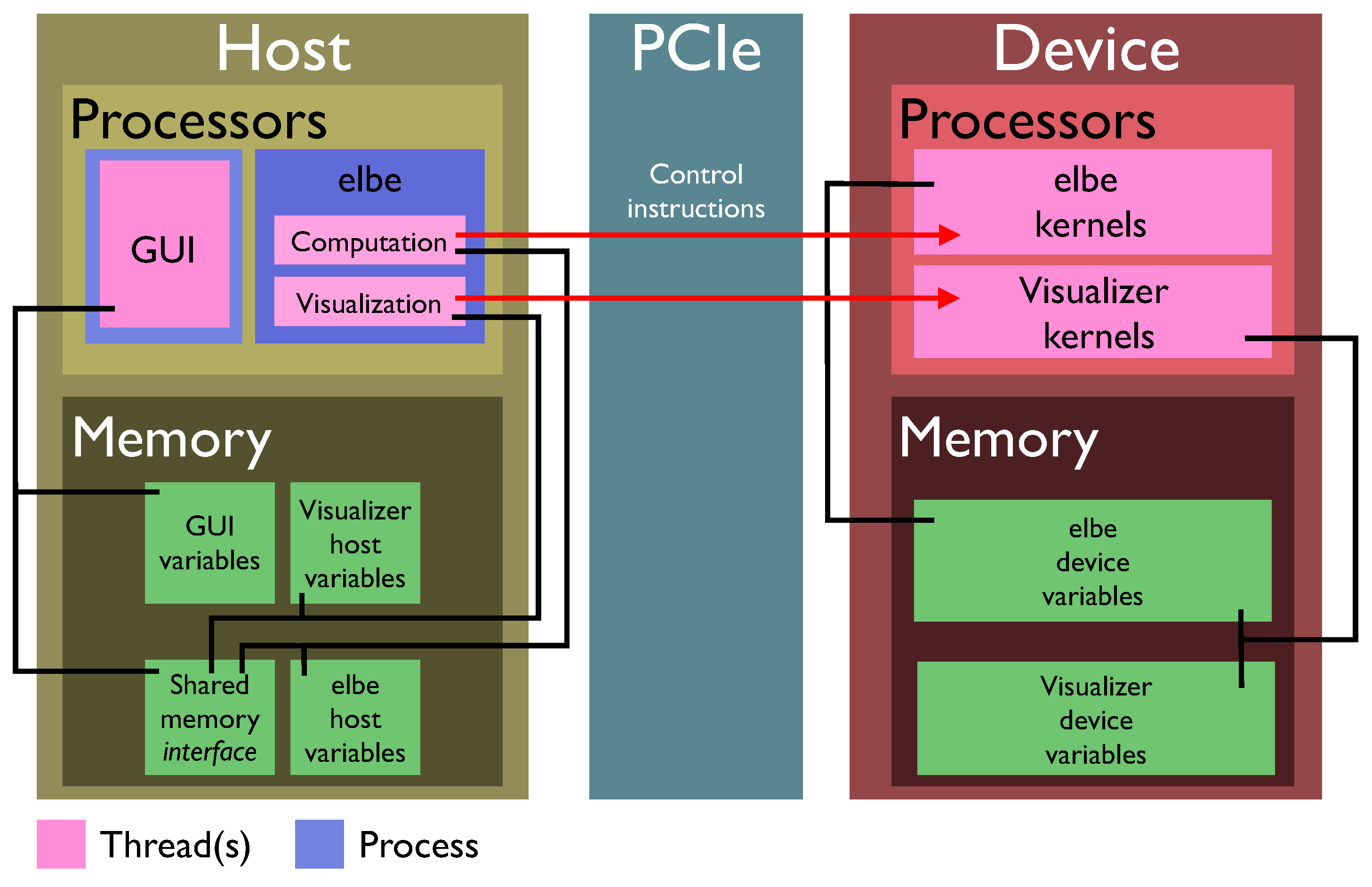
The main concern for the development of an adequate design philosophy was the inherent thread independence of computation and visualization. Generally, depending on the resolution of the simulation, the number of computed time steps per second varies dramatically. For the visualizer, a steady 20 rendered frames per second guarantee responsiveness to user-specified input. The presented design philosophy employs a multi-threaded approach for the instructional loops running on the host processors to control the GPU computation and visualization independently. This allows a constant stream of rendered frames, even under heavy computational load. Assuming that the visualization procedures are executed in an instant, a waiting period of 50 milliseconds results in the targeted 20 frames per second while also guaranteeing a slot in the GPU instruction queue for computational procedures.

Figure 4. Outline of the elbevis and graphical user interface instructions and execution, as well as memory handling.

Figure 4. Outline of the elbevis and graphical user interface instructions and execution, as well as memory handling.

Since the OpenGL buffer objects are mapped to the CUDA memory space, providing the desired pointers, the visualizer can access the computation’s variables at any point in time and render them to the screen in the manner of the applied visualization features. Both computation and visualization are executed in the same elbevis process, but as independent CPU threads. In order to provide a suitable control environment for the user, a graphical user interface (GUI) has been designed. The GUI is executed as an entirely independent process. To communicate with and instruct the computation/visualization, a shared memory segment is spawned by the elbevis process upon its start and connected with the GUI on request. The communication interface controls the entirety of the visualizer, i.e., by enabling the visualizer to toggle in the shared memory segment through the graphical user interface, the visualization thread is initiated. Thus, by turning off the visualizer, all that remains is the computation itself running at full capacity. In this state, the visualizer does not occupy any resources or computation time. Upon request by the GUI, the visualizer thread is spawned and awaits feature instructions read from the shared memory segment. Figure 4 depicts a schematic overview of the host and device processes/threads and memory organization.

4.2.1. OpenGL-CUDA Interoperability

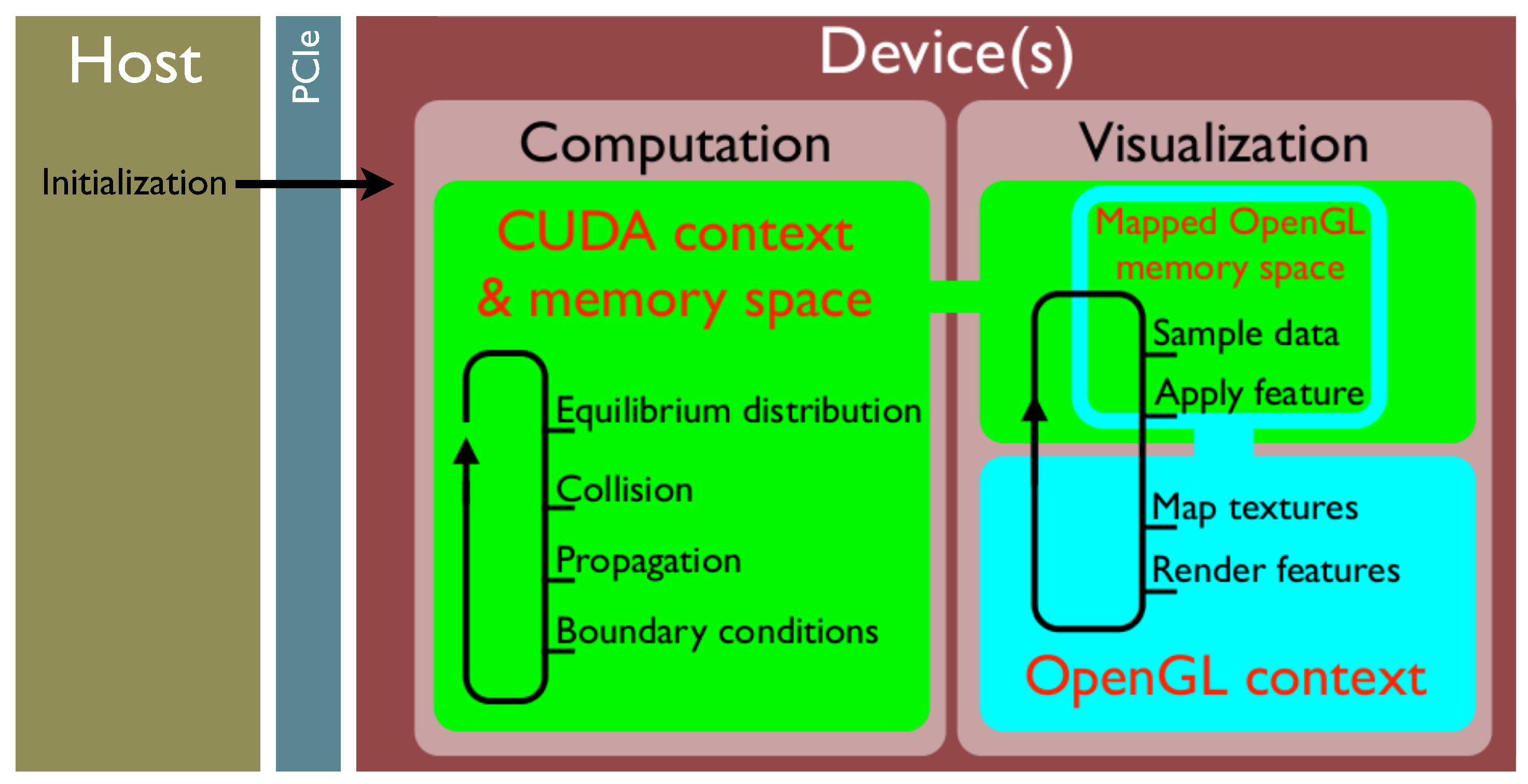
To explore OpenGL’s capability of rendering data directly from device memory, a buffer object has to be created, registered as a resource with CUDA and mapped to the CUDA address space. A pointer to the mapped buffer can then be used in CUDA kernels to read, write and modify the device data. The mapped OpenGL memory space can be thought of as a pointer that appears to the CUDA context as pointing to a CUDA address, but is actually tunneling to the OpenGL context in which it resides. A buffer object library has been designed in an effort to simplify the extensive use of buffer objects for OpenGL ↔ CUDA interoperability. Listing 1 provides a basic example of its use.

Listing 1: Basic example of the use of the buffer object library.

1 $\mathrm{\#include}\mathrm{ ″bufferobject.h″}$
2
3 $\mathrm{int}$ main() {
4 $\mathrm{// Setup CUDA and OpenGL}$
5 setup();
6 $\mathrm{// Create a new vertex buffer object, specifying the kind and the number of elements}$
7 BufferObject *vbo = $\mathrm{new}$ BufferObject (GL_ARRAY_BUFFER, nElements);
8 $\mathrm{// Get a mapped pointer to use with CUDA}$
9 $\mathrm{float}$ *dev_ptr = ($\mathrm{float}$*) vbo->getDevicePointer();
10 $\mathrm{// Do the CUDA computations}$
11 cudaKernel<<<blocks, threads>>>(dev_ptr);
12 $\mathrm{// Free the pointer so it can be used by OpenGL}$
13 vbo->doneWithDevicePointer();
14 $\mathrm{// Bind the buffer with OpenGL}$
15 vbo->bind();
16 $\mathrm{// Use the currently bound buffer for drawing}$
17 drawWithOpenGL();
18 $\mathrm{// Unbind the buffer}$
19 vbo->unbind();
20
21 $\mathrm{return}$ 0;
22 }
		     

4.2.2. CPU Multithreading

To decouple visualization and computation, they are executed in two separate threads. The portable operating system interface for UNIX (POSIX) threads, or pthreads, are used to realize the multi-threaded design. The traditional main loop is replaced by a pthread call to start the computation’s main loop in a separate thread. Subsequently, the so-called communicator loop is started, awaiting instructions from the control interface to initiate the visualizer thread. The SDLhandler and Visualizer objects are local variables of the visualizer thread and are allocated and deallocated with the thread’s initiation and termination, respectively. Pthreads’ built-in join functionality is used to guarantee controlled termination of all threads. POSIX is fully portable to the MAC OS X environment, but has very limited portability to Microsoft Windows. An alternative thread management library will have to be utilized to obtain major cross-platform compatibility in future elbevis versions.

4.3. Data Handling and the Sampling Methodology

The visualization in the discussed project is based on a sampling method. From the multitude of data available from the computation, a subset is copied to a mapped buffer object. The sampled data can either be written to a texture and then rendered as a quad primitive’s surface or be further processed with CUDA visualization routines before the rendering steps. Figure 5 depicts the computation and visualization loops and summarizes the mapping and rendering routines.

Figure 5. A schematic view of the OpenGL rendering process incorporated into the lattice Boltzmann implementation.

Figure 5. A schematic view of the OpenGL rendering process incorporated into the lattice Boltzmann implementation.

elbe does not support multi-GPU runs in a cluster environment yet. However, as a reference for future work, potential extensions of the proposed visualizer concept and sampling methodology to massively parallel simulations will be briefly discussed here. The primary driver to execute GPU accelerated code on clusters is the very limited amount of on-device DRAM memory, making it necessary to divide the domain of larger simulations into sub-domains, referred to as patches, and to assign these sub-domains to separate GPUs. A GPU cluster consists of two or more graphics devices ${\mathcal{D}}_{i,j}$ and one or more hosts ${\mathcal{H}}_i$. The communication speed between the devices depends on the provided data bus. The data transfer between the hosts is considerably slower than between the devices that share the same host environment, i.e., identical i index. Thus, data transfer limitations greatly incline, and the data transfer has to be limited the more indirect it is with regards to the device.

Real-time visualization on GPU clusters faces several challenges because of the data transfer and memory limitations. If the computation’s data are so large that they do not fit on one device, it is very likely that the data necessary for image processing also exceed the memory limit of the dedicated OpenGL device ${\mathcal{D}}_{i,j}^{*}$, i.e., the device with a monitor attached to it. Three alternative visualization approaches are presented and compared to handle the imposed limitations. The approaches are distinguished as dedicated and flexible device methods. For the dedicated device approach, ${\mathcal{D}}_{i,j}^{*}$ has fixed i and j indices, i.e., the monitor is always connected to the same device. This approach category is most suitable for single host GPU machines. The patch stitching method and the down sampling method are categorized as dedicated device approaches. An example for a flexible device approach where the i and j indices are changing is the patch visiting method.

The visualization work flow involves three essential steps: data sampling, the construction of visualizer features (like isolines) and the rendering of the feature. Depending on the applied visualization method, these steps are performed on one device (the dedicated OpenGL device ${\mathcal{D}}_{i,j}^{*}$) or split up and executed on separate devices.

The patch stitching method is a dedicated device approach. The unique dedicated OpenGL device ${\mathcal{D}}_{i,j}^{*}$ sequentially samples the data by accessing all computing devices (one at a time) and copying the relevant data subset to a mapped OpenGL vertex or pixel buffer object that is allocated on ${\mathcal{D}}_{i,j}^{*}$. It then constructs the visualizer feature for the sampled data and renders the result to the OpenGL device’s frame buffer. This procedure is repeated for each computing device’s data subset. According to the patch’s spatial location, the frame buffer is stitched together. Providing OpenGL pixel and vertex buffer objects for one computing device at a time reduces the memory requirements according to the total number of computing devices. The size of the frame buffer depends on the screen’s resolution and is therefore independent of the cluster size. The reasons for the application of a patch stitching method are the detailed feature construction and the strictly limited memory requirement. The downsides of the stitching method are the significant data transfer because the complete data subset scales with the domain size, the time lag that results while the data is copied and the feature’s patch independence requirement. The time lag is especially considerable if all stitches are supposed to be sampled at the same time step to avoid discontinuities at the reproduced patch borders. The patch independence requirement addresses the feature’s parallelization suitability. Entirely parallelized features, e.g., slice, isolines or vectors, are patch independent and can be constructed for a patch at a time; whereas features integrated in time or space, e.g., streamlines and streaklines, rely on patch communication and are therefore not suitable for a sequential rendering technique like the patch stitching method.

The down sampling method provides a mapped pixel and vertex buffer object of a prescribed size, independent of the domain size (as long as it does not exceed the domain size, in which case an up sampling method would have to be utilized). In accordance to the allocated memory for the buffer objects, a coarse subset of the relevant data subset is sampled from the computing devices, e.g., every fifth node value of a slice is copied to the vertex buffer object. After all of the data are assembled in the buffer objects, the visualizer feature is constructed and rendered to the frame buffer. Sampling all necessary data first and then performing the feature construction for the entire dataset makes this method suitable for all visualizer features. Adjusting the sampling density also changes the time needed for data copying. Therefore, the method is highly adaptable, and scenarios of variable sampling density are possible. For instance, consider a cluster computation of three computing devices and one dedicated OpenGL device. For most of the computation’s simulation time, the sampling density is extremely low, slowing down the main computation by a negligible amount. Upon the user’s request, e.g., holding the mouse button down, the sampling density is increased (almost stalling the main computation), and a high resolution image of the computation is rendered to the screen. With this method, the computation can be controlled throughout the entire simulation while providing detailed information whenever needed.

Patch visiting. The flexible device approach eliminates intra-device and intra-host communication entirely. All devices are computing devices with some memory to spare for visualization. The visualizer is started at the device in question and processes only the local data patch. The image rendered to the screen only visualizes the one patch’s variable field in full resolution. An obvious disadvantage of the patch visiting method is that information is limited to the device with the attached monitor. This method might be considered if a specific region of the domain is of special importance to the user. Consider the simulation of a ship where the pressure distribution on the bulbous bow (possibly limited to only a tenth of the entire domain) is significant for its dynamic shape optimization. In such a case, the visualization can be performed at full resolution and without any costly data transfers.

To conclude, real-time visualization on GPU clusters has to be constrained by either scope or resolution to avoid time-intensive data transfers. This is the case for the down sampling and the patch visiting approaches. The down sampling method should be preferred for cases where the entire domain is of importance, and the patch visiting method is ideal for cases where only a sub-domain is to be visualized. If the time aspect and high update rates are not important, the high resolution patch stitching method can be utilized to generate high resolution images of the entire domain. For now, elbe and elbevis only support simulations in a shared-memory multi-GPU environment with up to four GPUs and support the first preliminary implementations of the down sampling and patch visiting method. However, as multi-GPU simulations are beyond the scope of this work, this is not further investigated here.

4.4. Graphical User Interface

For the graphical user interface, the GTK+toolkit has been used, wrapped for C++ compatibility by the gtkmm extension package [32]. Two of the main reasons that lead to the decision of using the GTK+ environment over other GUI development APIs are the (1) unrestricted and comparatively easy portability to other platforms and (2) relative ease of use with the Glade GUI builder.

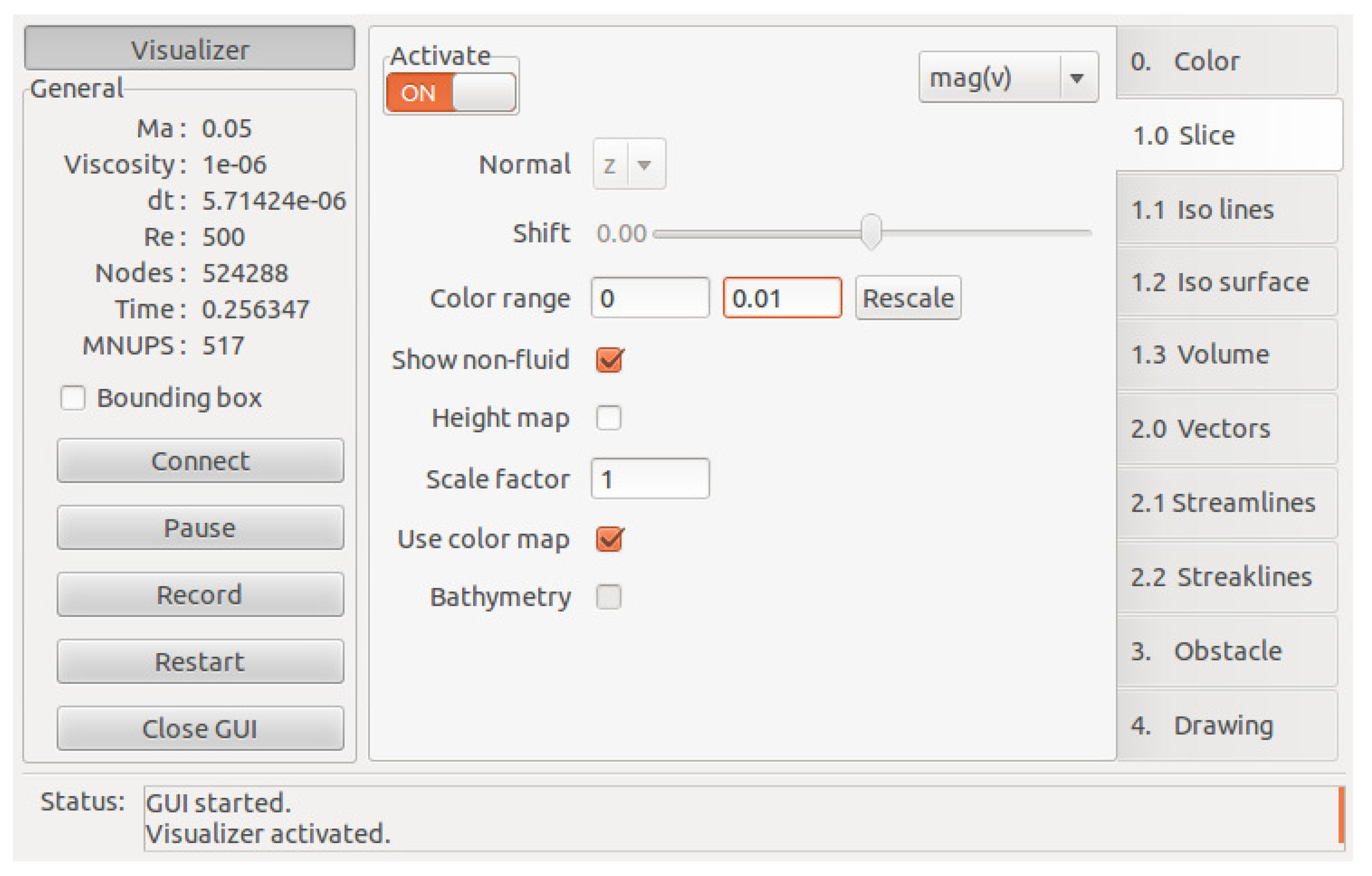
The layout of the GUI is divided into two main parts. The first is a general controls section applicable to overarching control and visualization features. These include, e.g., the start/stop functionality of the visualizer, displaying computational parameters (time step, grid size, viscosity, etc.) or pausing the computation. The second part regards the specific visualization features that will be discussed elaborately in Section 5. The specific features are activated by an on/off toggle button. Upon turning on/off a specific feature, the necessary memory allocation/deallocation is requested by setting the corresponding flag in the shared memory segment. The GTK+ GUI environment allows dynamic reorganization of selectable tree variables. Such variables are used to specify to which of the available and suitable variables the specific visualization feature should be applied. For example, consider the isosurface feature. Variables suitable for isosurface construction are inherently scalar variables or scalars derived from higher order variable fields. This includes such inherently scalar quantities as density or pressure and derived quantities like the velocity magnitude. Since some visualizer features can only be applied to either scalar or vector quantities, different selectable variable trees have to be built for each unique feature. Figure 6 shows the graphical user interface of elbevis with the active slice page.

Figure 6. Graphical user interface of the elbevis real-time visualization tool.

Figure 6. Graphical user interface of the elbevis real-time visualization tool.

4.4.1. Shared Host Memory Control Interface

As stated above, the graphical user interface is not part of the main computational process, thus not having any information about the computation’s variables readily available. The GUI had to be designed in such a way that it can be used for various simulations with a varying set of variables. To this end, basic variable information, like variable symbol (e.g., p for pressure), name, precision (integer, single precision, double precision) and kind (specifying scalar/vector), is stored in the shared memory segment and then used by the GUI to derive the selectable tree structures for each feature. The desired variable for the considered feature is chosen by means of a combo box from the variables available in the tree structure.

The cross-platform compatible boost inter-process library is used to generate, manage and access a shared memory segment in which the control interface is stored. The control interface collects all information necessary for communication between the graphical user interface process and the elbevis process. In the interface, entire variables are stored as opposed to storing pointers to variables, because each process has its own address space. Once a computation is started, a shared memory segment is created. The GUI can then be used to connect to the control interface and change the stored variables according to the user’s input.

The control interface is structured in a simulation and a visualization part. The simulation part stores information like the node number, the origin coordinates or the current simulation time. The visualization part is much more extensive and contains all of the features’ control variables, e.g., flags to activate/deactivate the feature, numeric values for parameters, like the iso value for isosurfaces or lines or each feature’s selected variable ID. The main computation’s field variables are enumerated and can be specified by the variable ID. The control interface’s structure allows easy access to control parameters.

The code snippet in Listing 2 creates a variable pointer and the control interface and accesses the interface to set the number of nodes in the x direction and the number of isolines.

Listing 2: Example of how to configure the interface.

1 $\mathrm{// Define a new vector variable and assign it the}$
2 $\mathrm{// name ″Velocity″ and the short name or symbol ″v″}$
3 Variable velocity (VECTOR, $\mathrm{″Velocity″},\mathrm{″v″}$);
4
5 $\mathrm{// Assign data pointers for the visualizer}$
6 velocity.data0D = ($\mathrm{void}$*) xVelocityDevicePtr;
7 velocity.data1D = ($\mathrm{void}$*) yVelocityDevicePtr;
8 velocity.data2D = ($\mathrm{void}$*) zVelocityDevicePtr;
9
10 $\mathrm{// Define an array of variables}$
11 Variable *variablesPtr [1] = &velocity;
12
13 $\mathrm{// Define the interface and initialize it with the numVariables (here, just one)}$
14 $\mathrm{// stored in the variablesPtr array}$
15 Interface interface(variablesPtr, numVariables);
16
17 $\mathrm{// Access the simulation part and specify the number of nodes in the x direction}$
18 interface->sim.nx = numNodesInX;
19 interface->vis.isoLinesNumber = 10;
		     

4.5. User Interaction

User interaction is essential for the generality of the developed real-time visualization tool. A number of different applications require very different analysis tools, point of views and dynamic rearrangement of the applied features. This sort of user interaction is considered interaction with the visualization and is further discussed in Section 4.5.1. Another kind of user interaction is the direct control of the computation itself, i.e., changing the actual simulation behavior according to real-time user input; this will be discussed in Section 4.5.2.

4.5.1. Interactive Monitoring

The most obvious tool for control and interaction with the visualization is the graphical user interface explained in Section 4.4, i.e., dynamically changing a slice position, isosurface value, color map, etc. Additional relevant interaction is realized by mouse or keyboard input. The presented implementation uses the Simple DirectMedia Layer (SDL) development library for low level access to not only the mouse and keyboard, but also the OpenGL setup. The SDL library has been chosen because of its cross-platform compatibility (supporting Windows, MAC OS X and Linux, among others), extended user input device access, and current widespread use and support. Opposed to the OpenGL Utility Toolkit (GLUT) as one of the most widespread alternatives, the SDL framework supports multi-threading and, most importantly for the developed visualizer, is not constrained to a main rendering loop, but can be executed on request. In elbevis, all SDL functionality is encapsulated in the SDLHandler library.

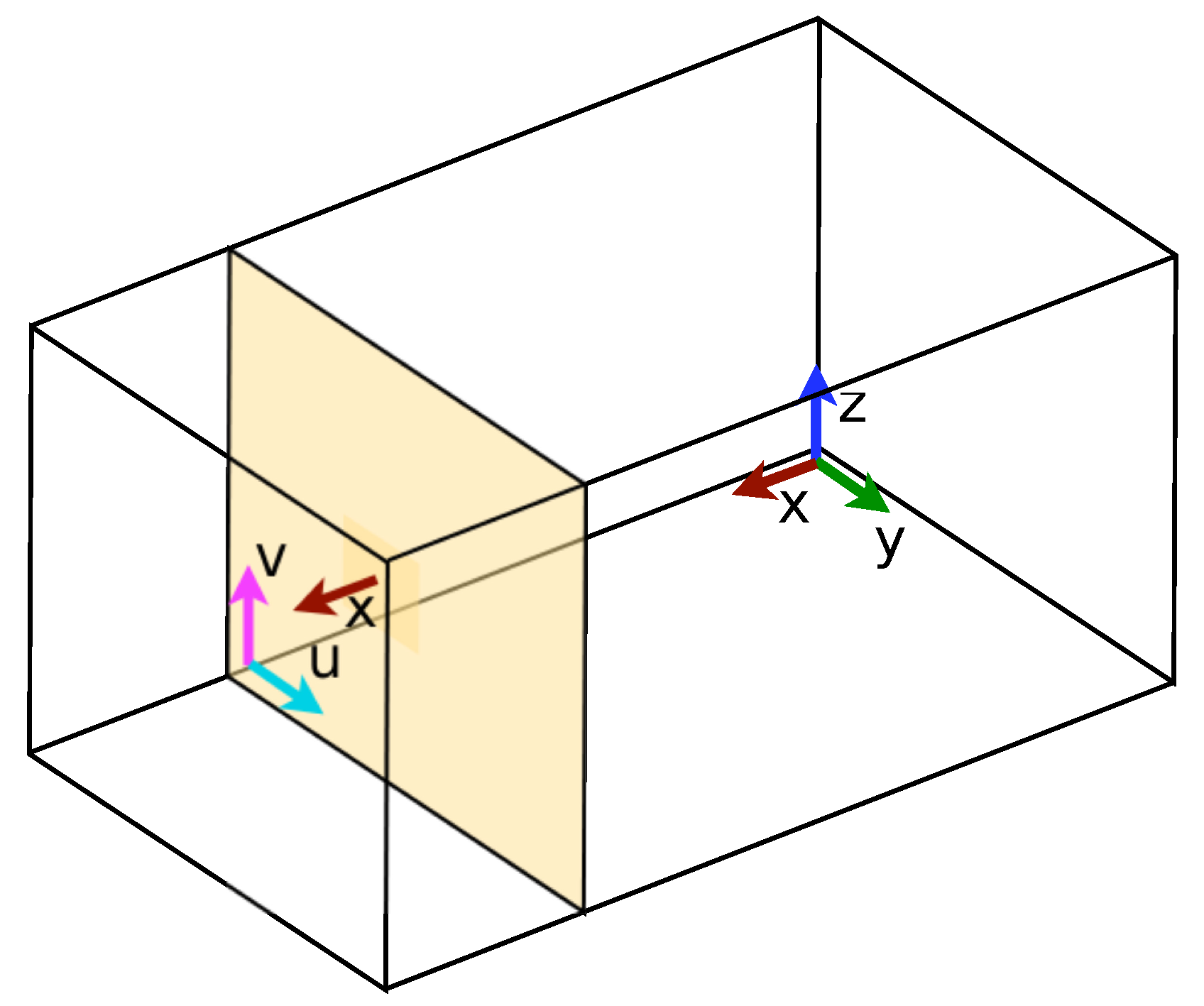
Examples for mouse input are panning, orbiting and zooming functionality within the rendered window. Keyboard inputs are used to switch between perspective and parallel projection. By pressing the x, y and z key, the view is aligned along the corresponding axes and parallel projection is activated. Pressing the key again restores the perspective projection and adjusts the zoom factor to fit the viewing spectrum that was obtained through parallel projection.

Scrolling the mouse wheel changes the applied zoom factor. A zooming effect can be acquired by either changing the distance to the shown object or by adjusting the viewing angle. Here, the latter is used. The OpenGL camera system corresponds to a right-handed coordinate system where the view direction is oriented along the z axis, x to the right, and y defines the up direction. Accordingly, the field of view can be defined by an opening angle in the $y,z$ plane. Scrolling the mouse wheel affects the opening angle and updates the perspective projection. By definition of a characteristic angle, the zooming behavior is non-linear for constant angle increments. Thus, for very low viewing angles, the increment is significantly reduced.

Panning and orbiting the displayed scene is implemented by transforming the desired panning vector and the current viewing normal, respectively. The window system has its origin in the upper left-hand corner with the window x-axis pointing to the right and the window y-axis pointing down. The desired window-pan $p_{\text{window}}={\left(p_x,-p_y,0\right)}^T$ has to be transformed to the simulation’s coordinate system through multiplication with the inverse of the model view matrix’s rotational part ($MV{M}_{\text{rot}}$), i.e., $p_{\text{simulation}}=MV{M}_{\text{rot}}^{-1}{p}_{\text{window}}$. For rotation, the window’s x- and y-axes are transformed to the simulation’s coordinate system with the same procedure, and the entire scene is rotated in two successive rotations around the obtained axes.

4.5.2. Interactive Steering

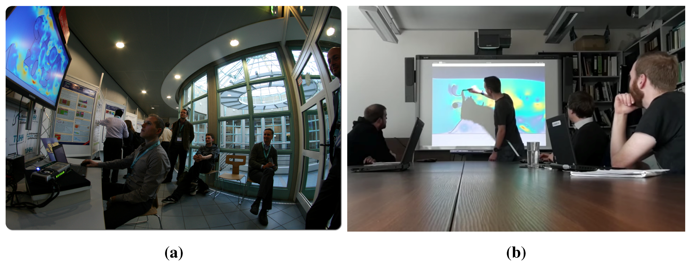
One of the interactive steering features implemented in elbevis is a drawing feature that can be activated for two-dimensional simulations. It allows the user to draw and remove no-slip walls in the fluid domain using the mouse cursor. This feature is representative for the interaction possibilities that lie within reach. Currently, further interaction with the computation is limited to stalling the simulation with the GUI’s pause button for detailed investigation of a given moment in time. Future interaction features could include drawing in 3D, mouse-controlled movement of objects and the adjustment of simulation parameters, like Mach number, grid spacing, viscosity, etc. Some parameter changes imply reinitialization of the field and reallocation of the memory, i.e., a profound alteration of the computation’s setup, making it difficult to implement.

5. Visualizer Features

The visualizer features are discussed in the following and exemplified with two standard fluid dynamics test cases, the Kármán vortex street (2D) and a dam break setup (3D): The Kármán vortex street is simulated as a two-dimensional single-phase channel flow around a cylinder. The computational domain has 1024 × 512 lattice nodes; the top and bottom domain boundaries are modeled as no-slip walls, and the cylinder is positioned at a quarter of the domain’s length in the upstream direction in-between the top and bottom wall. A dam break test case is used to demonstrate the three-dimensional visualizer features. The computational domain consist of $256\times 64\times 96$ lattice nodes; all lateral sides of the domain are modeled as no-slip boundary conditions, and a free surface module using the volume of fluid (VoF) method is utilized to simulate a collapsing vertical block of fluid. In the initial setup, a fluid film covers the bottom boundary of the domain, while a vertical block of fluid on one end of the domain covers a side wall. The fluid block’s height is slightly less than the domain height; it is extending to a quarter of the domain’s length, and covers all of the domain’s width.

5.1. Data Sampling

Computational domains of arbitrary size can be difficult to handle for visualization. Some visualizing routines might be very computationally or memory intensive for such cases. Thus, a data sampling method provides a way to apply certain features to just a subset of the entire data field. In general, an OpenGL pixel buffer object is used in a sampling routine to transfer the specific dataset that is to be visualized. The source data are sampled along an axis-aligned plane, i.e., constant i, j or k value. For the two-dimensional case, all data are visualized, and the slice coordinates resemble the domain coordinates. In the more general three-dimensional case, the slice is of variable size, according to the slice’s normal vector. The slice coordinates u and v are introduced with $n_u$ and $n_v$ slice nodes in the respective direction. Indices r and s are counting along u and v, respectively. Figure 7 depicts the slice’s coordinate system in relation to the computational orientation. The sampled data can now be processed to generate a variety of visualizer features.

Figure 7. Data sampling: 3D computational domain and 2D slice.

Figure 7. Data sampling: 3D computational domain and 2D slice.

5.2. Visualizer Features for Scalar Quantities

Several visualizer features were designed to simplify the interpretation of scalar data. Some of the presented features are limited to 2D use only, such as isolines and height map.

5.2.1. Colored Slice

Whenever a dataset is to be colored, a certain color map has to be used to translate the quantity’s value to a four-component color. A color in the RGBA space is characterized by its red, green, blue and alpha value. The presented method uses a unity mapping method in which any data value ϕ is shifted by the dataset’s assumed minimum value ${\varphi }_{min}$ and scaled by the set’s respective data range width ${\varphi }_{max}-{\varphi }_{min}$. Data values within $\Phi =\{{\varphi }_{min}:{\varphi }_{max}\}$ are mapped to $I=\{0:1\}$, and values outside Φ will also exceed I’s limits. Thus, to generate an adequate color for a data value, all color maps range from zero to one. One of the most widely-used color maps is the rainbow map ranging from blue to green to red. This map is implemented by piece-wise linear functions for all color channels. The local functions:

$$c\left(\tilde{x}\right)=\left\{\begin{array}{cc}0\hfill & |\tilde{x}|>1\hfill \\ 1\hfill & |\tilde{x}|<\frac{1}{3}\hfill \\ 1.5(1-|\tilde{x}\left|\right)\hfill & \text{else}\hfill \end{array}\right.c=r,g,b$$

with the local variables:

$$\tilde{x}=2\frac{x-x_{\text{mid}}}{c_w}=2\frac{x-c_s}{c_w}-1c=r,g,b$$

are used to blend the colors in and out, where $x_{\text{mid}}$ is the center point of the respective color’s distribution and $c_w$ and $c_s$ are the color’s width and start point, respectively. See Figure 8 for the local function and the color distributions that result from:

$$c_s=\left\{\frac{1}{3},0,-\frac{1}{3}\right\}\text{and}{c}_w=\{1,1,1\}$$

Figure 8. Local and global color functions for the rainbow/default color map.

Figure 8. Local and global color functions for the rainbow/default color map.

It is sometimes desirable to have a transparent fading effect on the lower end of the data range. For this effect, the alpha channel is utilized. It is defined as:

$$a(r,g,b)=\left\{\begin{array}{cc}1\hfill & r+g+b>1\hfill \\ r+g+b\hfill & r+g+b\le 1\hfill \end{array}\right.$$

This definition results in a transparent fading effect for data values below the minimum assumed range value. For some visualization applications, only part of the assumed data range should be colored with non-transparent color values. Such an effect is realized by the compression factor $\chi \in \{0:1\}$, which modifies each color channel’s width and start value with ${\widehat{c}}_w=c_w(1-\chi )$ and ${\widehat{c}}_s=c_s+\chi (1-c_s)$. Figure 9 shows the effect of $\chi =0.625$ resulting in $b_s=0.5$; the alpha channel is depicted in gray. In addition to the color functions stated above, the red color channel in this case is set to one for x values exceeding the maximum assumed range.

Figure 9. Effect of the color compression factor $\chi =0.625$ and transparent blending.

Figure 9. Effect of the color compression factor $\chi =0.625$ and transparent blending.

An alternative way to define color maps is the four-point model. At positions $x_i=\left\{0,\frac{1}{3},\frac{2}{3},1\right\}$, the colors $c_i$ are prescribed. A linear interpolation between the $x_i$ then yields the overall color distribution. For the rainbow color distribution, the adequate set of colors would be:

$$\begin{array}{cc}\hfill r_i& =\{0,0,1,1\}\hfill \end{array}$$

(1)

$$\begin{array}{cc}\hfill g_i& =\{0,1,1,0\}\hfill \end{array}$$

(2)

$$\begin{array}{cc}\hfill b_i& =\{1,1,0,0\}\hfill \end{array}$$

(3)

Figure 10 depicts the five color maps implemented in elbevis and shows the two different color map definitions with their respective transparent fading effects. The four-point model’s five color maps are shown at the bottom, and the rainbow color maps’ transparent fading effect is compared for the four-point model (second from top) and the local-color-function model (top).

Figure 10. Color map definitions in elbevis.

Figure 10. Color map definitions in elbevis.

Once the color map is applied to every node of the slice, it is bound to a texture and rendered onto a quad primitive. The slice feature is one of the most efficient tools, since the only processing step besides the data sampling is the coloring of the field, while also being one of the most versatile to convey the flow’s behavior. Figure 11a depicts a colored slice of the velocity magnitude colored with the rainbow color map, blue for slow and red for fast. Similarly, Figure 11b shows the transparently-colored slice applied to the velocity magnitude field of the dam break test case. Regions of very low velocity are rendered transparently to obtain color values only for regions where fluid is present.

Figure 11. Colored slice applied to the two- and three-dimensional example flows. (a) 2D flow around a cylinder; (b) 3D dam break flow.

Figure 11. Colored slice applied to the two- and three-dimensional example flows. (a) 2D flow around a cylinder; (b) 3D dam break flow.

5.2.2. Height Map

A rubber sheet can be used to visualize two-dimensional scalar fields in the third dimension. According to the scalar’s value, a height map is generated, where the height is defined as being perpendicular to the 2D scalar field. To provide a linear approximation, triangles are utilized to resemble the surface elevation. Each vertex is assigned a color in accordance to its relative variable value for the field’s data range. Alternatively, the surface normals necessary for shading and light computations are derived from the field’s gradient obtained with the central differencing scheme for each node. The surface normals are:

$${\tilde{n}}_{ij}=s_{x,ij}\times s_{y,ij}$$

(4)

where:

$$\begin{array}{cc}\hfill s_{x,ij}& ={(2\Delta x,0,{\varphi }_{i+1j}-{\varphi }_{i-1j})}^T\hfill \end{array}$$

(5)

$$\begin{array}{cc}\hfill s_{y,ij}& ={(0,2\Delta x,{\varphi }_{ij+1}-{\varphi }_{ij-1})}^T\hfill \end{array}$$

(6)

are the slope vectors depicted in Figure 12. This yields:

$${\tilde{n}}_{ij}=\left(\begin{array}{c}2\Delta x\\ 0\\ {\Delta }_x\varphi \end{array}\right)\times \left(\begin{array}{c}0\\ 2\Delta x\\ {\Delta }_y\varphi \end{array}\right)\propto \left(\begin{array}{c}{\varphi }_{i-1j}-{\varphi }_{i+1j}\\ {\varphi }_{ij-1}-{\varphi }_{ij+1}\\ 2\Delta x\end{array}\right)$$

for the normal direction. The normalized surface normal $n_{ij}=\frac{{\tilde{n}}_{ij}}{|{\tilde{n}}_{ij}|}$ is then used for the OpenGL shading pipeline.

Figure 12. Slope vectors for normal derivation on height map surfaces.

Figure 12. Slope vectors for normal derivation on height map surfaces.

5.2.3. Isolines

The computation and display of isolines is a very common feature in visualizing tools. The challenge in this particular case was to design a method that can be efficiently executed in parallel on the device, with device data. The methodology used in the present work is based on a dissection of the computational grid, to assign independent domain sub-areas to parallel threads. First, the grid is divided into squares, and each CUDA kernel thread on the device is assigned a square in such a way that every square is assigned exactly once. At this point, a marching squares algorithm [33] could be used to generate the isolines. It uses squares with weights on each corner to construct lines connecting interpolated iso points on the square’s edges. This algorithm differentiates $2^4=16$ different interpolation cases, necessitating look-up tables to find the right case for the found scenario. For this thesis, an alternative approach using triangles has been designed in an effort to simplify the method and to avoid look-up tables. The main advantage of using triangles instead of squares is that the three points of a triangle uniquely define a plane, whereas squares, or more accurately, in the case of weight quads, can be folded along their diagonal, defining two planes. The definition of just one unique plane with the triangle method renders look-up tables needless.

An isoline CUDA kernel function uses the sampled source vertex buffer object (vbo) and a target vertex buffer object to generate the contour lines from the raw slice data. As mentioned above, each kernel has an assigned square of four data points. The squares are divided into two triangles along the northeast diagonal, which are then deformed in such a way that their domain perpendicular elevation corresponds to the data value stored at its corner points. As mentioned above, the advantage of using triangles compared to squares is that a triangle can only have one intersecting line with a plane (the plane of the iso level in this case). Therefore, the triangle’s sides can be individually tested for plane intersection. The stretching of the triangles to match the data values is equivalent to a linear data interpolation along the grid lines. Hence, a linear approximation is used to find the intersecting point coordinates. Since any triangle can only pierce through the iso level plane once or not at all, the algorithm should find two or no line intersections for each triangle tested. In case there has been an intersection detected, the actual isoline is drawn from one line intersection to the other. The target vbo for the entire isoline has to be of a size:

$$s=n_{sq}·2·2·\mathsf{dim}·\mathtt{s}\mathtt{i}\mathtt{z}\mathtt{e}\mathtt{o}\mathtt{f}(\mathsf{precision})$$

where $n_{sq}$ is the number of squares. Each square has two triangles; each triangle might intersect the iso level plane, generating a line of two points, whereof each point has $\mathsf{dim}$ coordinate entries of size according to their precision.

Figure 13a shows a stretched triangle (orange) piercing through the iso level plane (transparent grey). Grid points of the considered triangle with a sampled data value of less than the iso value are depicted in blue; those with a value of more than the iso value are shown in red; any others are colored black. Two of the triangle’s sides have end points on opposite sides of the iso level plane. Along these purple triangle edges, the data are interpolated, and the intersection point (bright green diamonds) is determined. The bright green line connecting the diamonds marks the isoline segment for the triangle in question. Due to the northeast dissection of the grid, an asymmetry of sub-grid resolution is introduced, as seen in Figure 13b’s depiction of the most basic contour line case of one high point being symmetrically surrounded by low points. The considered iso value in this example is set to be the mean of the highest and lowest points. The solid black line is an intuitive first-guess best approximation representing a possible exact solution. The basic marching squares algorithm would result in the dashed isoline. The area circumscribed by the marching squares line is half of the estimated exact area, the shape replicated but rotated by an angle of ${45}^{\circ }$. The triangulated grid approach yields a solution closer to the estimated exact solution in both area and deviation from the exact lines, but cannot replicate the symmetry. Figure 13c exemplifies a more realistic scenario of arbitrary value elevations for the presented method. Note that the introduced asymmetry only affects the far northeast and southwest ends of the detected line, leading to a better approximation in some cases, e.g., the northeast end of the small crest.

Figure 13. Isoline generation with a triangulated grid approach and linear interpolation. (a) A stretched triangle piercing through the iso level plane. Linear stretching yields linear data interpolation. (b) For a simple point-symmetric case, the triangulated method introduces asymmetries of sub-grid resolution. (c) Isolines generated with the triangulated grid approach for a realistic value elevation field.

Figure 13. Isoline generation with a triangulated grid approach and linear interpolation. (a) A stretched triangle piercing through the iso level plane. Linear stretching yields linear data interpolation. (b) For a simple point-symmetric case, the triangulated method introduces asymmetries of sub-grid resolution. (c) Isolines generated with the triangulated grid approach for a realistic value elevation field.

Figure 14. Isolines applied to a flow around a cylinder at $Re=500$.

Figure 14. Isolines applied to a flow around a cylinder at $Re=500$.

In fluid mechanics, isolines can be constructed to easily quantify the velocity magnitude field and clearly define regions within a given magnitude interval. In Figure 14, ten homogeneously-incremented isolines are applied to the flow field’s entire range of velocity magnitudes.

5.2.4. Isosurface

The three-dimensional equivalent of an isoline is an isosurface. The simplistic triangulated grid approach cannot be transferred to 3D; an external library for a CUDA-based marching cubes algorithm is therefore utilized [34]. The marching cubes algorithm splits the grid into cubes and determines surface triangles depending on the cube’s eight corner data values. Each corner can either be within (less than) or outside (greater than) of the isosurface (the iso value). Thus, $2^8=256$ unique cases have to be accounted for. A look-up table is used to find the matching case followed by interpolations to determine the exact polygon intersections. A bit of an eight-bit integer variable is reserved for each corner to compute the look-up ID of the considered cube. The GPU’s low latency texture memory is utilized to speed up the computation and to reduce the number of clock cycles for the look-up table access.

Figure 15a shows a surface dynamically determined with the marching cubes algorithm. The isosurface feature has been used to construct and render the fluid’s free surface from the VoF’s fill level variable computed for every lattice node. The isosurface feature can not only be used to reconstruct the free surface, but can also be applied to the velocity or density field to acquire information about values within the fluid.

Figure 15. Extended visualization: (a) Example of a free-surface dynamically computed with the marching cubes algorithm; (b) Volume rendering applied to the dam break’s velocity magnitude field.

Figure 15. Extended visualization: (a) Example of a free-surface dynamically computed with the marching cubes algorithm; (b) Volume rendering applied to the dam break’s velocity magnitude field.

5.2.5. Volume Rendering

For some application cases, it is desirable to gather information about field quantities throughout the entire domain. For a complex fluid flow problem, it might be relevant to find those specific three-dimensional areas in which a certain velocity or pressure value is exceeded. To obtain this information, a volume rendering procedure is implemented. All domain nodes are rendered transparently in accordance to a user-specified color map.

This implementation of a pseudo volume rendering was chosen to make the fundamental building blocks of the LB method visible. The user can see every node of the lattice that is relevant for his investigations; as opposed to traditional slice/texture or ray casting-based volume rendering techniques, where a domain sampling or reconstruction would hide the nature of lattice nodes. It should be noted, though, that traditional volume rendering techniques would be far more capable at producing realistic renderings, including shading. Various high quality, efficient and hardware-accelerated volume renderers have been implemented by Krüger [35], Stegmaier [36] and Stuart [37].

In the case of velocity magnitudes, this yields node clouds of points within a defined velocity range. Nodes with velocities below the prescribed range are discarded with an OpenGL alpha test function. In the current implementation, this cut-off value is set to one percent of the user-specified maximum opacity of the nodes. Discarding points of especially low opacity is essential for the performance. With this method, only a subset of all points is rendered at all, whereas without it, all points of the domain would have to be rendered (colored, blended, fragmented, depth tested). Values within the color range are (i) colored according to the current color map and the defined data range and (ii) transparently blended according to the defined data range and maximum opacity. The points that exceed the data range can either be truncated or colored with the upper color map value and the maximum opacity.

For complex three-dimensional fluid flow problems, the visualization of field values throughout the entire domain can be very useful. Figure 15b shows the dam break’s velocity magnitude distribution. Lattice nodes are transparently blended with their opacity and color adjusted in accordance to the applied data range and color map. Lattice nodes with vanishing velocities are discarded entirely.

5.3. Visualizer Features for Vector Quantities

Several visualizer features were designed to simplify the interpretation of vector data.

5.3.1. Vector Glyphs

Vector glyphs visualize a given vector field at sampled locations. A vector glyph representing the velocity field can be thought of as an elastic, yet rigid in its bending moment, flag that extends according to the velocity’s magnitude and adapts its orientation according to the stream. The flag’s seed or sample point represents its pivoting point and indicates the flow direction at the seed point’s location. Since the computational domain’s resolution is much higher than a reasonable resolution for the vector grid, sub-sampling is necessary. Consider the two-dimensional case: for a grid of $n_x\times n_y$ computation points and a vector spacing of $d_{nV}$ computation grid points between every two vector seeds, the total number of vector seeds is $n_{Vx}·n_{Vy}$, with:

$$n_{Vx}=\frac{n_x-1-\frac{d_{nV}}{2}}{d_{nV}}+1\text{and}{n}_{Vy}=\frac{n_y-1-\frac{d_{nV}}{2}}{d_{nV}}+1$$

using integer division. For a computational domain with a single ghost layer surrounding the main grid, the mapping of vector coordinates ($i_V$ and $j_V$) to grid coordinates (i and j) reads:

$$i=d_{nV}/2+i_V·d_{nV}+1\text{and}j=d_{nV}/2+j_V·d_{nV}+1$$

in the x and y direction, respectively. Figure 16 shows the relations stated above applied to an example with $n_x=10,ny=5,d_{nV}=3$.

Figure 16. Mapping of vector coordinates to grid coordinates.

Figure 16. Mapping of vector coordinates to grid coordinates.

The vector at $i_V,j_V$ represents the velocity at $i,j$. Thus, the first point of the vector line $V_{i_V,j_V}$ is at $x_{ij}$, and the second point is at:

$$x_{ij}+l·\frac{u_{ij}}{|u_{ij}|}\text{where}l=\frac{|u_{ij}|}{{\left|u\right|}_{\text{max}}-{\left|u\right|}_{\text{min}}}$$

where is the length of the vector and $u_{ij}$ is the velocity at $x_{ij}$.

Vector glyphs can be used to convey a sense of the flow field’s direction and magnitude. Constructing a vector for every twentieth lattice node generates the rendering depicted in Figure 17a. Longer vectors in the cylinder’s wake indicate high streaming velocities, while very short vectors represent low streaming velocities. The vector spacing is set to twenty lattice nodes, and the vector length is normalized by the applied spacing. The vector’s rotation clearly indicates the rotary motion of fluid particles in the oscillating flow regime.

Figure 17. Vector visualizer feature. (a) Vectors applied to a flow around a cylinder at $Re=500$; (b) Vectors applied to the dam break’s velocity field.

Figure 17. Vector visualizer feature. (a) Vectors applied to a flow around a cylinder at $Re=500$; (b) Vectors applied to the dam break’s velocity field.

The vector feature can also be applied to a three-dimensional flow and produces the image depicted in Figure 17b for the flow’s velocity field. The slice’s red regions are now shown as long vector lines, whereas they disappear for the transparent parts of the slice.

5.3.2. Streamlines

Streamlines originate at seed points and follow the velocity vector field or, more generally, any given vector field. Streamlines represent the flow field of a time instance and can be constructed by step-wise integration of the considered field values. For a vector field ${\varphi }_{ij}$, a streamline of $N_{\text{stream}}$ points can be constructed with the following sequential algorithm. Because of the algorithm’s sequential nature, a parallelization is realized in the concurrent integration of multiple streamlines. The streamline S’s $i_s$-th element is calculated with:

$$S_{i_s}=S_{i_s-1}+{\varphi }_{ij\left(S_{i_s-1}\right)}·\Delta s$$

with $i_s=\{1,2,...,N_{\text{stream}}-1\}$, the stream step size $\Delta s$ and the seed point $S_0=x_{\text{seed}}$. The function $ij\left(S_{i_s-1}\right)$ represents a mapping from the continuous x space to the discrete $i,j$ space. With the definition of the origin $x_o$ at the first non-ghost node, the following mapping can be applied:

$$ij\left(x\right)=\left\{i\right(x),j(y\left)\right\}$$

$$i\left(x\right)=1+\frac{x-x_o}{\Delta x},j\left(y\right)=1+\frac{y-y_o}{\Delta x}$$

where x and y are the dimensional components of any x.

Figure 18. Streamlines applied to a flow around a cylinder for different Reynolds’ numbers. (a) $Re=30$; (b) $Re=500$.

Figure 18. Streamlines applied to a flow around a cylinder for different Reynolds’ numbers. (a) $Re=30$; (b) $Re=500$.

Figure 19. Streamlines. (a) Streamlines applied to a flow around a cylinder at $Re=500$ (entire domain); (b) Streamlines applied to the dam break’s velocity field.

Figure 19. Streamlines. (a) Streamlines applied to a flow around a cylinder at $Re=500$ (entire domain); (b) Streamlines applied to the dam break’s velocity field.

In Figure 18, two visualizer features are applied. A slice feature is utilized to show the geometry of the cylinder, and streamlines originating in the cylinder’s wake are used to show the circulating flow field and the surrounding stream. For a low Reynolds’ number of $Re=30$, the observed flow stays laminar with two circulating flow regimes on the back side of the cylinder. For $Re=500$, turbulent separation occurs, and an oscillating flow field develops. Figure 18 shows a close up view of the cylinder’s wake. The result of streamlines applied to the entire domain is shown in Figure 19a. The three-dimensional equivalent, the application of streamlines to the dam break velocity field, is shown in Figure 19b.

5.3.3. Streaklines

A streakline is the line that would be drawn by ink injected into the flow. Therefore, this line evolves and grows over time. With each time step, all existing points are translated according to the current velocity at that point, and an additional point is added to the line of points. Consider a streakline $X^0$ of length k forming $k-1$ line segments:

$$X^0=\{x_0,x_1,x_q,...,x_{k-1}\}$$

For parallel, explicit integration in time, a second streakline vector $X^1$ is used. Two pointers $X^{\text{new}}$ and $X^{\text{old}}$ are then used to swap back and forth between $X^0$ and $X^1$. Both, $X^{\text{new}}$ and $X^{\text{old}}$ are initialized with points at $x_{\text{fo}}$ far outside of the computational domain. For every time-step, each of the now old streakline’s elements is locally integrated in time in parallel threads q:

$$x_q^{\text{old}}\leftarrow x_q^{\text{old}}+u_{ij\left(x^{\text{old}}\right)}·n_{\text{vis}}·\Delta t$$

where $n_{\text{vis}}$ is the number of computational time steps that occurred since the streakline procedure was executed the last time. As a next step, the number of points to add to the streakline $n_{\text{add}}$ is determined by:

$$n_{\text{add}}=\frac{|x_{\text{seed}}-x_0^{\text{old}}|}{\Delta x}·n_{\text{seeds/dx}}+1$$

where $n_{\text{seeds/dx}}$ is defined as the seed density. The translated points are then transferred to $X^{\text{new}}$ with a q-shift of $n_{\text{add}}$:

$$x_q^{\text{new}}\leftarrow x_{q-n_{\text{add}}}^{\text{new}}\text{for}q\ge n_{\text{add}}$$

The additional seed points are added to the first $n_{\text{add}}-1$ elements:

$$x_q^{\text{new}}\leftarrow \frac{q}{n_{\text{add}}}\left(x_{\text{seed}}-x_0^{\text{old}}\right)\text{for}q<n_{\text{add}}$$

See Figure 20 for an example where a directionally-oscillating velocity field results in a sinusoidal streakline.

Figure 20. A streakline evolving over time.

Figure 20. A streakline evolving over time.

The different features presented above have one thing in common: they all represent the flow field for a single instance in time and cannot depict the flow’s history. Especially for transient flows, a tool conveying the simulation’s history can be desirable. Streaklines are integrated over time and visualize the movement of fluid particles. In the case of the Kármán vortex street, this feature produces the familiar alternating and spreading vortices. Figure 21 shows a streakline generated by injecting tracking particles immediately behind the cylinder and convecting them with the flow. The shown rendering was captured after a quasi-stationary flow developed and enough particles were convected to the end of the domain.

Figure 21. Streakline applied to a flow around a cylinder at $Re=500$.

Figure 21. Streakline applied to a flow around a cylinder at $Re=500$.

5.4. Surface Mapping

If obstacles are introduced to the flow, it is desirable to acquire knowledge about certain field variable values at the considered obstacle’s surface. Therefore, a surface mapping feature uses the normals of the obstacle’s surface mesh triangles to sample the variable field. Each node of each triangle has its own normal vector, resulting in three independent color values for each triangle. The projection of a scalar field ${\varphi }_{ijk}$ to a mapped value ${\varphi }_{\text{mapped},q}$ at vertex q with unit normal vector $n_q$ is implemented as follows:

$${\varphi }_{\text{mapped},q}={\varphi }_{ijk}(q,n)$$

with:

$$\widehat{i}:={(\widehat{i},\widehat{j},\widehat{k})}^T={(\mu ,\mu ,\mu )}^T+\frac{q-O}{\Delta x}$$

and:

$$i=\left\{\begin{array}{cc}\widehat{i}+1\hfill & n_x>0\hfill \\ \widehat{i}\hfill & n_x\le 0\hfill \end{array}\right.j\text{and}k\text{accordingly}$$

where O is the domain’s origin and μ is an offset factor that depends on the number of ghost layers applied to the simulation. OpenGL’s vertex coloring procedures are used to interpolate the triangle’s color along the edges and also for the triangle area. This feature can be used to visualize the pressure distribution along an obstacle’s surface to convey a sense for high-load regions of the considered body. The grid generator can be used to add arbitrary objects, in this case a sphere, to the dam break test case. The resulting flow is shown in Figure 22a with the isosurface feature applied to the fill level variable. To convey a sense for the pressure distribution and, therefore, the loads acting on the body’s surface, the surface mapping feature can be used. The result is shown in Figure 22b.

Figure 22. Example of the surface mapping feature: (a) A spherical obstacle is added to the computational domain of the dam break test case; (b) The flow’s density distribution on the obstacle’s surface colored with the rainbow color map.

Figure 22. Example of the surface mapping feature: (a) A spherical obstacle is added to the computational domain of the dam break test case; (b) The flow’s density distribution on the obstacle’s surface colored with the rainbow color map.

5.5. Performance

The performance of elbevis is summarized in Table 1 and Table 2 for the two test cases that were introduced earlier in this section: the Kármán vortex street (2D, $1024\times 512$ lattice nodes) and a dam break setup (3D, $256\times 64\times 96$ lattice nodes). The simulations were run on a recent NVIDIA GTX Titan board in an off-the-shelf workstation. The computational performance is normalized to the performance of a standalone elbe run without active visualizer features. For the 2D case, a very low impact of the visualization on the code performance can be observed: the average performance is around 90%–95% of the elbe bulk performance. However, the isoline filter and the streamline filter dramatically decrease performance, as expected: both visualizer features introduce a large additional overhead that can hardly be parallelized. In 3D, the results are very similar: the performance reduction is around $5\%$, even for the very complex isosurface filter. The performance results clearly proof the applicability and efficiency of the proposed visualizer concept, including complex three-dimensional flows with a free surface.

Table 1. Performance of scalar filters for a 2D and 3D LBM kernel, in relation to the performance of elbe without any visualizer features activated.

Test Case	No Filter	Scalar Filters
		Slice	Isolines	Isolines + Slice	Isosurface	Volume Rendering
Kármán vortex street (2D)	$100\%$	$95\%$	$78\%$	$76\%$	-	-
Dambreak (3D)	$100\%$	$96\%$	-	-	$93\%$	$96\%$

Table 1. Performance of scalar filters for a 2D and 3D LBM kernel, in relation to the performance of elbe without any visualizer features activated.

Test Case	No Filter	Scalar Filters
		Slice	Isolines	Isolines + Slice	Isosurface	Volume Rendering
Kármán vortex street (2D)	$100\%$	$95\%$	$78\%$	$76\%$	-	-
Dambreak (3D)	$100\%$	$96\%$	-	-	$93\%$	$96\%$

Table 2. Performance of vector filters for a 2D and 3D LBM kernel, in relation to the performance of elbe without any visualizer features activated.

Test Case	No Filter	Vector Filters
		Glyphs	Glyphs + Slice	Streaklines	Streaklines + Slice	Streamlines
Kármán vortex street (2D)	$100\%$	$99\%$	$95\%$	$92\%$	$88\%$	$38\%$
Dambreak (3D)	$100\%$	-	-	-	-	-

Table 2. Performance of vector filters for a 2D and 3D LBM kernel, in relation to the performance of elbe without any visualizer features activated.

Test Case	No Filter	Vector Filters
		Glyphs	Glyphs + Slice	Streaklines	Streaklines + Slice	Streamlines
Kármán vortex street (2D)	$100\%$	$99\%$	$95\%$	$92\%$	$88\%$	$38\%$
Dambreak (3D)	$100\%$	-	-	-	-	-

6. Applications

The previously-presented visualizer tool now can be applied to diverse flow problems of different kinds. The elbe code features 1D, 2D and 3D computing kernels with different physics, ranging from shallow water flow models (solving for depth-averaged Navier–Stokes equations) to full Navier–Stokes models, including the effects of viscosity and turbulence. Two-dimensional applications are certainly more impressive in terms of run-times, as both the amount of grid nodes and the complexity of the computations are lower, compared to the three-dimensional models. In the following, a 2D interactive test case will be presented first. The model even allows for interactions with the user to change and/or control the flow characteristics and is very responsive in terms of computational times. Afterwards, three-dimensional applications for the visualizer toolkit will be shown.

6.1. Interactive 2D elbevis Playground

Due to the minimally-invasive concept and the high performance of the numerical solver, elbevis allows for very responsive interactions between the user and the numerical simulation. In Figure 23a, the presentation of elbevis at the 2013 GACM (German Association for Computational Mechanics) colloquium on computational mechanics in Hamburg is shown, for a 2D application case with simple inlet/outlet boundary conditions on the left/right end of the computational domain. Note that the simulation is run on an NVIDIA GTX Titan board that is attached to an off-the-shelf laptop through an ExpressCard slot. The user now can control the visualization by selecting the desired visualizer features, color maps, and so on. On top, the computational domain can be modified by freely drawing shapes, e.g., GACM 2013 in the example below. The effects on the flow field, including information on the high speed regions, local circulation and pressure, can immediately be observed.

Figure 23. elbevis playground in action: (a) During the poster session at the GACM 2013 conference in Hamburg, Germany; (b) In a typical classroom situation on a smart board.

Figure 23. elbevis playground in action: (a) During the poster session at the GACM 2013 conference in Hamburg, Germany; (b) In a typical classroom situation on a smart board.

6.2. Real-Time Simulations in 3D: A380 Cabin Mock-Up

Following the interactive two-dimensional show cases, as a first real-world application of the flow solver, the numerical simulation of aerodynamics inside an A380 cabin mock-up is analyzed. Such flow simulations are of great interest when addressing the thermal comfort of the passengers during the design of the cabin ventilation system. Figure 24a shows a sample mock-up configuration that also served as the basis for the experimental work of [38]. Due to the relatively small test case dimensions and the low inflow velocity, the numerical simulation of internal aerodynamics could be realized in real time, on a ten million node grid and while watching the transient evolution of flow patterns in elbevis. The simulation of 10 minutes of real time took approximately 10 min. The above-mentioned computational setup with an external GTX Titan board in a ViDock expansion chassis was used.

Figure 24. Application of elbevis to an A380 cabin mock-up. (a) Geometry, including six rows of passengers; (b) Volume rendering of the corresponding velocity field. Inlets in the ceiling and the suction outlets in the bottom part of the cabin can clearly be seen.

Figure 24. Application of elbevis to an A380 cabin mock-up. (a) Geometry, including six rows of passengers; (b) Volume rendering of the corresponding velocity field. Inlets in the ceiling and the suction outlets in the bottom part of the cabin can clearly be seen.

6.3. Further 3D Applications

Apart from these interactive real-time applications, elbevis can also be used for simulations that run near real-time, as the visualizer still allows one to control the simulation progress and to analyze the flow field characteristics. Some sample applications that have been recently analyzed with elbevis are:

• In the simulation of turbulent mixing in a complex 3D stirring unit, the numerical task was to optimize the shape and position of the stirring unit blades with respect to a maximized free surface area that controlled the efficiency of the chemical reaction under consideration (Figure 25a).
• Similarly, elbevis helped to control the numerical analysis of aircraft ditching. This test case was found to be very sensitive to a proper test case setup, so that a continuous monitoring of the numerical simulation during the first stages of the simulation was very helpful (Figure 25b).
• As the third and last test case, elbevis was used during the simulation of the external aerodynamics of a formula student race car [39] to test several different car under-body configurations (Figure 25c).

All three applications could benefit from the innovative visualizer concept, which allowed interactively monitoring the simulations, without time-consuming file-I/O and subsequent visualization with CPU-based visualizer tools.

Figure 25. Further applications of elbe and elbevis: (a) Visualization of the turbulent mixing in a complex 3D stirring unit (b) Numerical analysis of aircraft ditching; (c) external aerodynamics of the formula student racer EGN 2014 [39].

Figure 25. Further applications of elbe and elbevis: (a) Visualization of the turbulent mixing in a complex 3D stirring unit (b) Numerical analysis of aircraft ditching; (c) external aerodynamics of the formula student racer EGN 2014 [39].

7. Conclusions and Outlook

We presented the implementation of an integrated visualizer tool for the real-time visualization of complex two- and three-dimensional flow problems. Thanks to the minimally-invasive software concept, the visualization does not interfere with the numerical simulation, and no impact on computational performance was observed. Moreover, the simulations can be launched without a visualizer interface, which can be turned on during later stages of the numerical simulation through a shared memory interface. The data exchange between simulation and the visualizer is realized with shared OpenGL-CUDA memory spaces. Depending on the selected visualizer feature, a subset of data is extracted from the CUDA data arrays and further processed in the visualizer. Here, our own CUDA-implemented visualizer filters are applied.

The simulation also allows for multi-GPU simulations. However, the direct benefit of no performance degradation vanishes, as the data have to be transferred to the visualizing GPU first, before the subsequent filtering and data preparations can take place. This will be further improved in future work.

Similarly, the whole concept is based on locally-installed GPUs, as the standard OpenGL implementations do not feature remote rendering yet. With the presented expansion chassis configurations and external GPUs, this is of minor importance. However, this is a limiting factor as soon as GPU clusters are involved. Future work will address this problem.

References

1. Kreylos, O.; Tesdall, A.; Hamann, B.; Hunter, J.; Joy, K. Interactive Visualization and Steering of CFD Simulations. In Proceedings of the Eighth Eurographics Workshop on Virtual Environments, Barcelona, Spain, 30–31 May 2002; pp. 25–34.
2. Höfler, M. Real-time Visualization of Unstructured Volumetric CFD Data Sets on GPUs. In Proceedings of the Central European Seminar on Computer Graphics for Students, Budměřice, Slovensko, 23–26 April 2006.
3. De Vuyst, F.; Labourdette, C.; Rey, C. GPU-Accelerated Real-Time Visualization and Interaction for Coupled Fluid Dynamics. Avaiable online: http://documents.irevues.inist.fr/handle/2042/52817 (accessed on 6 September 2015).
4. Janßen, C. elbe . Avaiable online: https://www.tuhh.de/elbe/home.html (accessed on 6 September 2015).
5. Tölke, J.; Krafczyk, M. TeraFLOP computing on a desktop PC with GPUs for 3D CFD. Int. J. Comput. Fluid Dyn. 2008, 22, 443–456. [Google Scholar] [CrossRef]
6. Linxweiler, J.; Krafczyk, M.; Tölke, J. Highly interactive computational steering for coupled 3D flow problems utilizing multiple GPUs. Comput. Vis. Sci. 2010, 13, 299–314. [Google Scholar] [CrossRef]
7. Delbosc, N.; Summers, J.; Khan, A.; Kapur, N.; Noakes, C. Optimized implementation of the Lattice Boltzmann Method on a graphics processing unit towards real-time fluid simulation. Comput. Math. Appl. 2014, 67, 462–475. [Google Scholar] [CrossRef]
8. Janßen, C.; Krafczyk, M. Free surface flow simulations on GPUs using the LBM. Comput. Math. Appl. 2011, 61, 3549–3563. [Google Scholar] [CrossRef]
9. Akenine-Moller, T.; Haines, E.; Hoffman, N. Real-Time Rendering; CRC Press/A K Peters, Ltd.: Natick, MA, USA, 2008. [Google Scholar]
10. Pharr, M.; Humphreys, G. Physically Based Rendering, Second Edition: From Theory to Implementation; Morgan Kaufmann Publishers Inc.: San Francisco, CA, USA, 2010. [Google Scholar]
11. Shreiner, D.; Sellers, G.; Kessenich, J.; Licea-Kane, B. OpenGL Programming Guide: The Official Guide to Learning OpenGL; Addison-Wesley Longman Publishing Co., Inc.: Upper Saddle River, NJ, USA, 2013. [Google Scholar]
12. Sellers, G.; Wright, R.; Haemel, N. OpenGL SuperBible: Comprehensive Tutorial and Reference; Pearson Education: Boston, MA, USA, 2013. [Google Scholar]
13. NVIDIA. NVIDIA’s Next Generation CUDA Compute Architecture: FERMI. Comput. Syst. 2009, 26, 63–72. [Google Scholar]
14. Kirk, D.; Hwu, W. Programming Massively Parallel Processors; Elsevier Inc., Morgan Kaufmann Publishers: Burlington, MA, USA, 2010. [Google Scholar]
15. Patterson, D.; Hennessy, J. Computer Organization and Design; Elsevier Inc., Morgan Kaufmann Publishers: Burlington, MA, USA, 2011. [Google Scholar]
16. Official NVIDIA C for Graphics (Cg) Website. Available online: https://developer.nvidia.com/cg-toolkit (accessed on 10 September 2015).
17. Kessenich, J.; Baldwin, D.; Rost, R. The OpenGL Shading Language; Language Version 4.50, Revision 5; The Khronos Group Inc.: Beaverton, OR, USA, 30 January 2015; Available online: https://www.opengl.org/registry/doc/GLSLangSpec.4.50.pdf (accessed on 10 September 2015).
18. Nickolls, J.; Dally, W. The GPU Computing Era. IEEE Micro 2010, 30, 56–69. [Google Scholar] [CrossRef]
19. Houston, M. GPU Architecture. University Lecture CS448S Topics in Computer Graphics: Beyond Programmable Shading (SIGGRAPH 2010). Available online: http://bps10.idav.ucdavis.edu/ (accessed on 10 September 2015).
20. Fernando, R. GPU Gems: Programming Techniques, Tips and Tricks for Real-Time Graphics. Dimensions 2001, 7, 816. [Google Scholar]
21. Pratx, G.; Xing, L. GPU computing in medical physics: A review. Med. Phys. 2011, 38. [Google Scholar] [CrossRef]
22. NVIDIA. CUDA C Programming Guide; Technical Report, PG-02829-001_v7.5; NVIDIA: Santa Clara, CA, USA, September 2015; Available online: http://docs.nvidia.com/cuda/pdf/CUDA_C_Programming_Guide.pdf (accessed on 10 September 2015).
23. Woolley, C. CUDA Overview. Developer Technology Group, NVIDIA Corporation. Available online: http://www.cc.gatech.edu/~vetter/keeneland/tutorial-2011-04-14/02-cuda-overview.pdf (accessed on 10 September 2015).
24. Intel Corporation. Intel 64 and IA-32 Architectures Optimization Reference Manual; Order Number: 248966-030; Intel Corporation: Santa Clara, CA, USA, September 2014; Available online: http://www.intel.de/content/dam/www/public/us/en/documents/manuals/64-ia-32-architectures-optimization-manual.pdf (accessed on 10 September 2015).
25. NVIDIA. CUDA Developer Website. Available online: https://developer.nvidia.com/cuda-zone (accessed on 10 September 2015).
26. Linxweiler, J. An Integrated Software Approach to Interactive Exploration and Steering of Fluid Flow Simulations on Many-Core Architectures. Ph.D. Thesis, Braunschweig University of Technology, Braunschweig, Germany, 2011. [Google Scholar]
27. Ikits, M.; Magallon, M. The OpenGL Extension Wrangler Library (GLEW). Available online: http://glew.sourceforge.net/ (accessed on 10 September 2015).
28. Khronos Group. Official OpenGL Website. Available online: https://www.khronos.org/opengl (accessed on 10 September 2015).
29. Bernsdorf, J. Simulation of Complex Flows and Multi-Physics with the Lattice-Boltzmann Method. Ph.D. Thesis, University of Amsterdam, Amsterdam, The Netherlands, 2008. [Google Scholar]
30. Janßen, C.; Grilli, S.; Krafczyk, M. Efficient simulations of long wave propagation and runup using a LBM approach on GPGPU hardware. In Proceedings of the 22nd Offshore and Polar Engineering Conference (ISOPE), Rhodes, Greece, 17–22 June 2012.
31. Janßen, C.; Grilli, S.; Krafczyk, M. A fast numerical method for internal flood water dynamics to simulate water on deck and flooding scenarios of ships. In Proceedings of the 32nd International Conference on Ocean, Offshore and Arctic Engineering (OMAE), Nantes, France, 9–14 June 2013.
32. gtkmm. C++ Interfaces for GTK+ and GNOME. Available online: http://www.gtkmm.org (accessed on 10 September 2015).
33. Maple, C. Geometric Design and Space Planning Using the Marching Squares and Marching Cube Algorithms. In Proceedings of the 2003 International Conference on Geometric Modeling and Graphics, London, UK, 16–18 July 2003.
34. Krone, J. GPU Particle-Grid Methods: Molecular Surfaces and Synthetic Density Maps. In Proceedings of the Workshop on GPU Programming for Molecular Modeling, Urbana, IL, USA, 6–8 August 2010.
35. Kruger, J.; Westermann, R. Acceleration techniques for GPU-based volume rendering. In Proceedings of the 14th IEEE Visualization 2003 (VIS’03), Seattle, WA, USA, 24 October 2003; p. 38.
36. Stegmaier, S.; Strengert, M.; Klein, T.; Ertl, T. A simple and flexible volume rendering framework for graphics-hardware-based raycasting. In Proceedings of the Fourth International Workshop on Volume Graphics, Stony Brook, NY, USA, 20–21 June 2005; pp. 187–241.
37. Stuart, J.A.; Chen, C.K.; Ma, K.L.; Owens, J.D. Multi-GPU volume rendering using MapReduce. In Proceedings of the 19th ACM International Symposium on High Performance Distributed Computing, Chicago, IL, USA, 21–25 June 2010; pp. 841–848.
38. Kühn, M.; Bosbach, J.; Wagner, C. Experimental parametric study of forced and mixed convection in a passenger aircraft cabin mock-up. Build. Environ. 2009, 44, 961–970. [Google Scholar] [CrossRef]
39. e-gnition Team Hamburg. Available online: http://egnition-hamburg.de/ (accessed on 10 September 2015).