
Use of CMEIAS Image Analysis Software to Accurately Compute Attributes of Cell Size, Morphology, Spatial Aggregation and Color Segmentation that Signify in Situ Ecophysiological Adaptations in Microbial Biofilm Communities

Abstract
:
1. Introduction
2. Descriptions of Unique CMEIAS Algorithms
2.1. Measurement of Microbial Body Size
2.1.1. Accurate Measurement of Cell Length and Width Using Shape-Adaptable Algorithms
2.1.2. Accurate Measurement of Biovolume Body Size Using Shape-Adaptable Algorithms
2.2. Rules of Pattern Recognition for Microbial Morphotype Classification
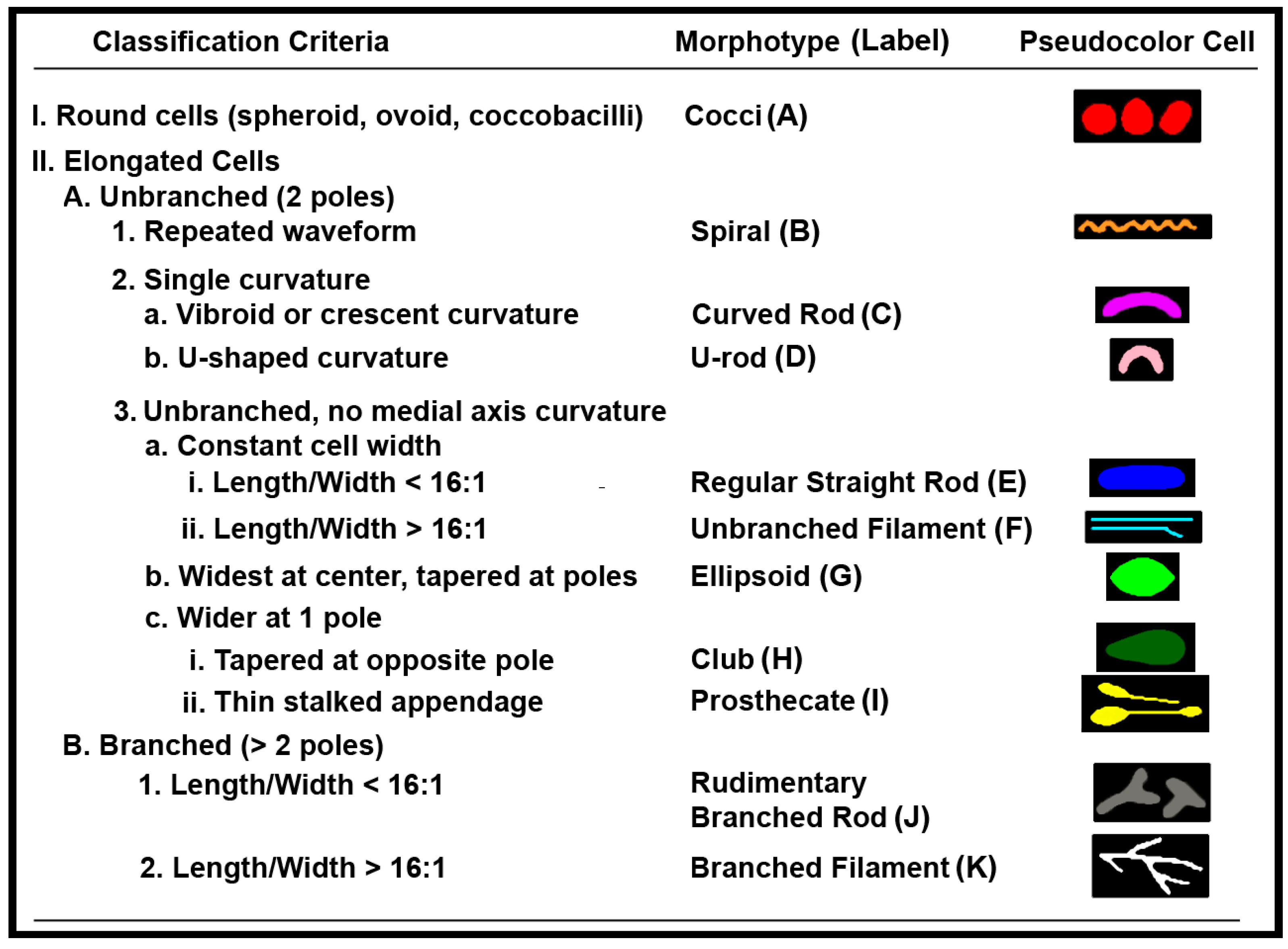
2.2.1. Rule () for Category A1
2.2.2. Rule () for Elongated Morphotypes
2.2.3. Rule () for Further Classification of Prosthecate Subcategory I1, Spiral Group B and Branched Filament Group K
2.2.4. Rule () for Spiral and Unbranched Filament Morphotypes
2.2.5. CMEIAS k-NN Morphotype Classifier
2.2.6. Importance of Fourier Descriptors in the Morphotype Classifier
2.3. Geospatial Pattern Analysis: CMEIAS Aggregation Cluster Index
2.4. Color Segmentation Algorithm
3. Application of These CMEIAS Algorithms for Analysis of in Situ Microbial Ecology
3.1. Sample Preparations
3.2. CMEIAS Image Analysis of the Microbial Biofilm Assemblages
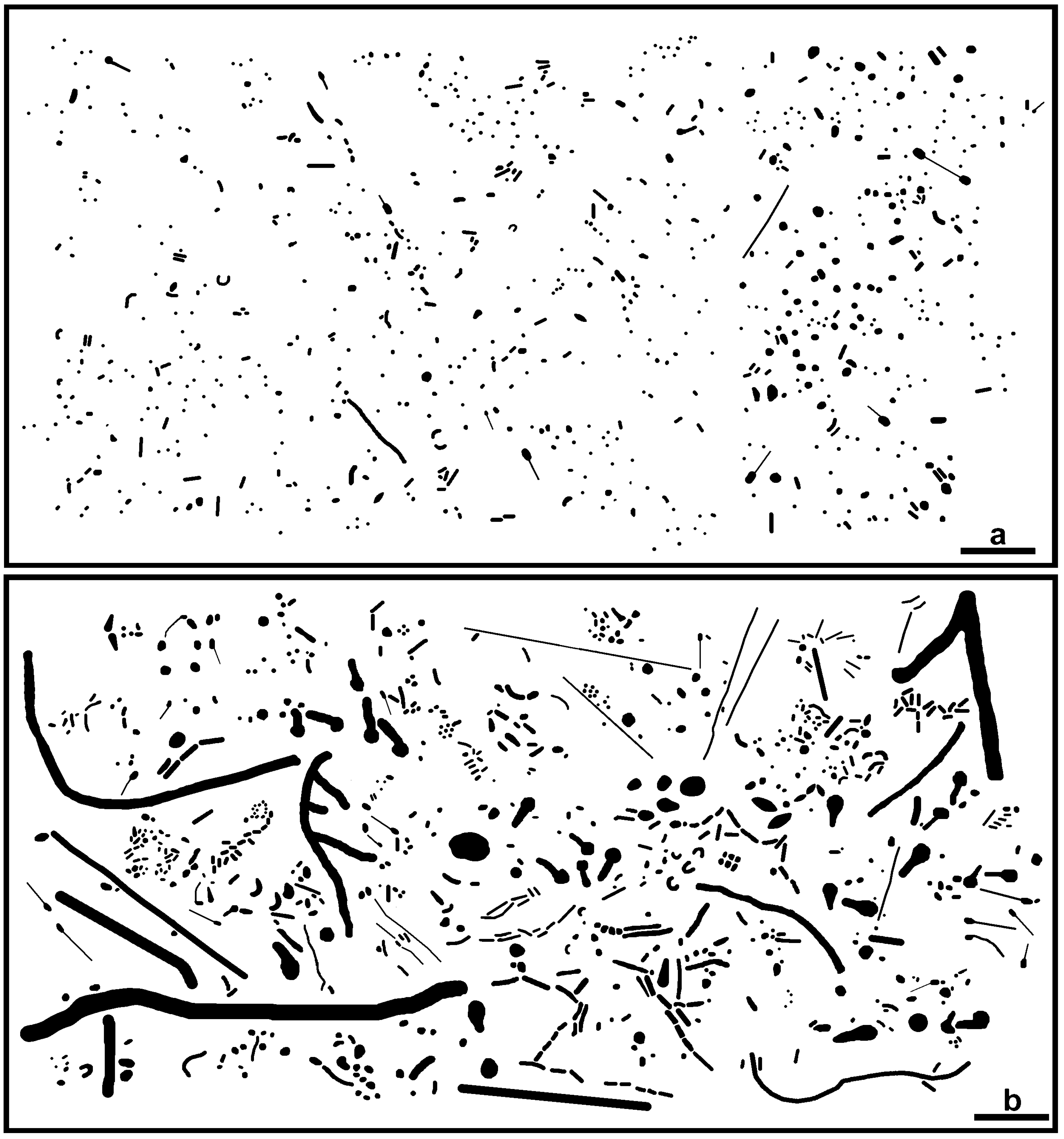
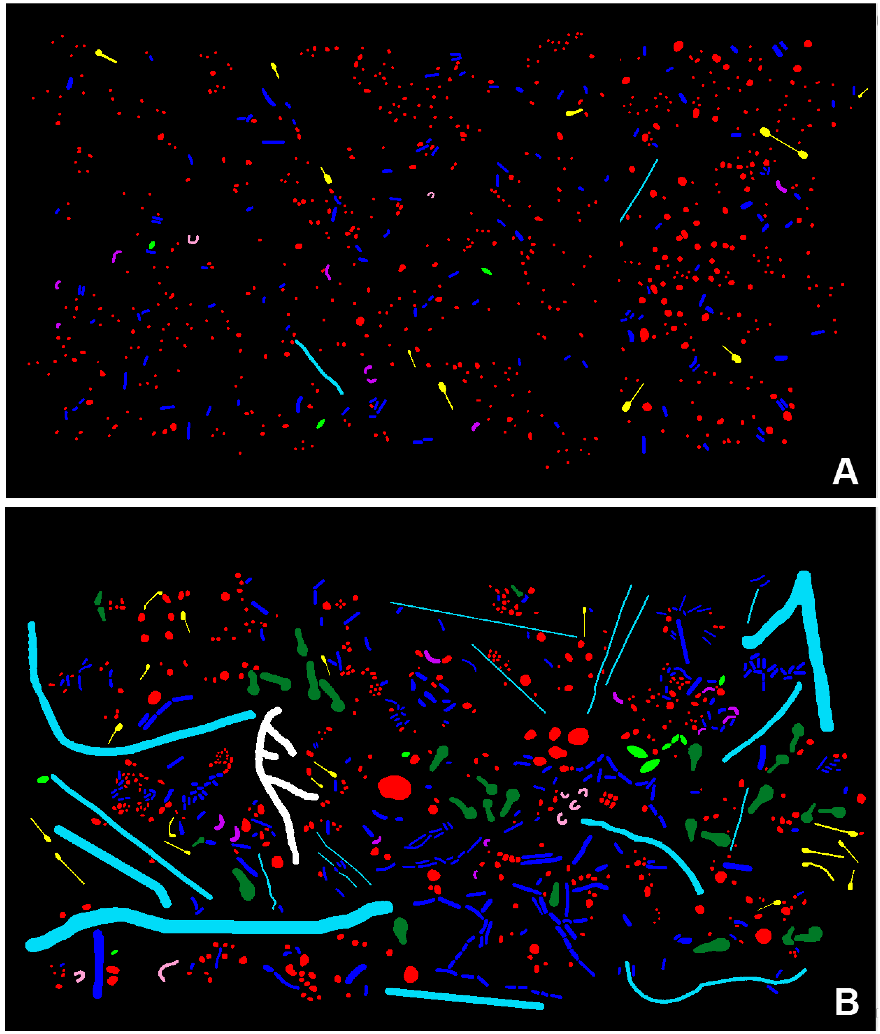
3.2.1. Morphological Diversity

| Morphotype/Eco-Statistic | Differential Cell Counts | Biovolume (µm3) | ||
|---|---|---|---|---|
| Assemblage A (Plain Glass) | Assemblage B (Polystyrene) | Assemblage A (Plain Glass) | Assemblage B (Polystyrene) | |
| Coccus | 620 | 413 | 104 | 260 |
| Curved Rod | 8 | 12 | 4 | 8 |
| U-shaped Rod | 2 | 5 | 1 | 4 |
| Regular Straight Rod | 115 | 255 | 45 | 151 |
| Unbranched Filament | 2 | 19 | 4 | 568 |
| Ellipsoid | 3 | 9 | 2 | 15 |
| Club | 0 | 28 | 0 | 171 |
| Prosthecate | 10 | 18 | 7 | 7 |
| Branched Filament | 0 | 1 | 0 | 50 |
| Totals | 760 | 760 | 166 | 1235 |
| Shannon Diversity | 0.610 | 1.160 a | 1.044 | 1.480 a |
| Simpson Diversity (1/D) | 1.453 | 2.439 a | 2.173 | 3.428 a |
| Berger–Parker’s Dominance | 0.816 a | 0.543 | 0.623 a | 0.460 |
| Smith and Wilson Evenness | 0.192 | 0.484 a | 0.395 | 0.560 a |
| Simpson Evenness | 0.208 | 0.271 a | 0.310 | 0.381 a |
| % Proportional Dissimilarity | 27.24% | 61.82% | ||
| Bray-Curtis Distance | 0.272 | 0.762 | ||
3.2.2. Filamentous Microbial Morphotypes as Related to Refuge from Protozoan Bacteriovory
3.2.3. Ecophysiological Attributes Linked to Accurate Measures of Biovolume Body Mass
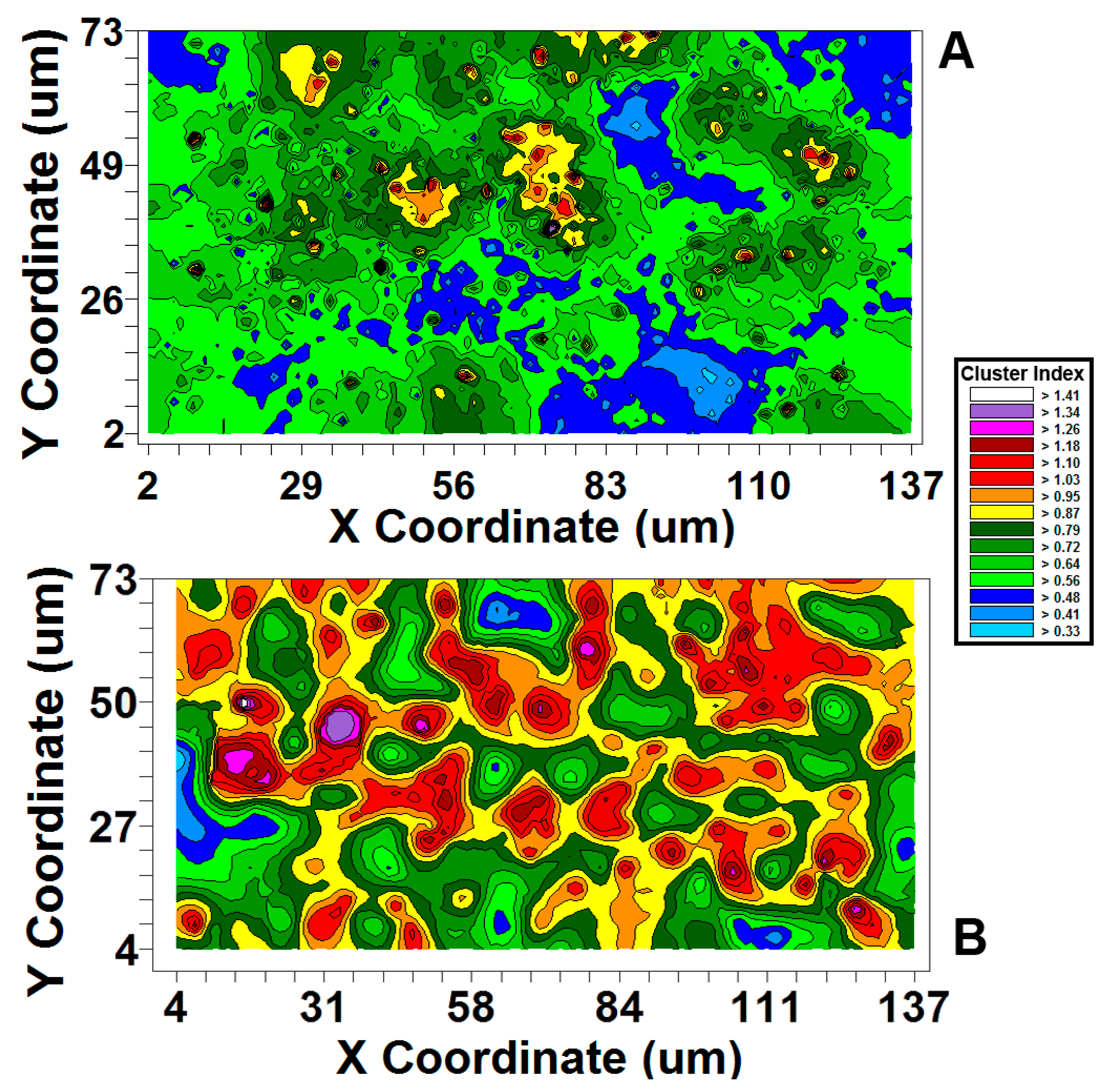
3.2.4. Spatial Pattern Analysis and Its Relationship to Microbial Biofilm Ecology
| Distribution Statistic | Plain Glass | Polystyrene | Interpretation of Aggregation |
|---|---|---|---|
| Range | 1.669 | 4.767 |  Polystyrene > Control Glass Polystyrene > Control Glass |
| Median | 0.636 | 0.725 |  Polystyrene > Control Glass Polystyrene > Control Glass |
| Mode | 0.976 | 1.574 |  Polystyrene > Control Glass Polystyrene > Control Glass |
| Maximum | 1.855 | 4.881 | Polystyrene > Control Glass |
| Shapiro–Wilk Normality Test W (p) | 0.935 (0) | 0.849 (0) | Distribution Not Normal |
| Mann–Whitney Median Test U (p) | 330,216 (1.30 × 10⁻⁶) | Polystyrene > Control Glass | |
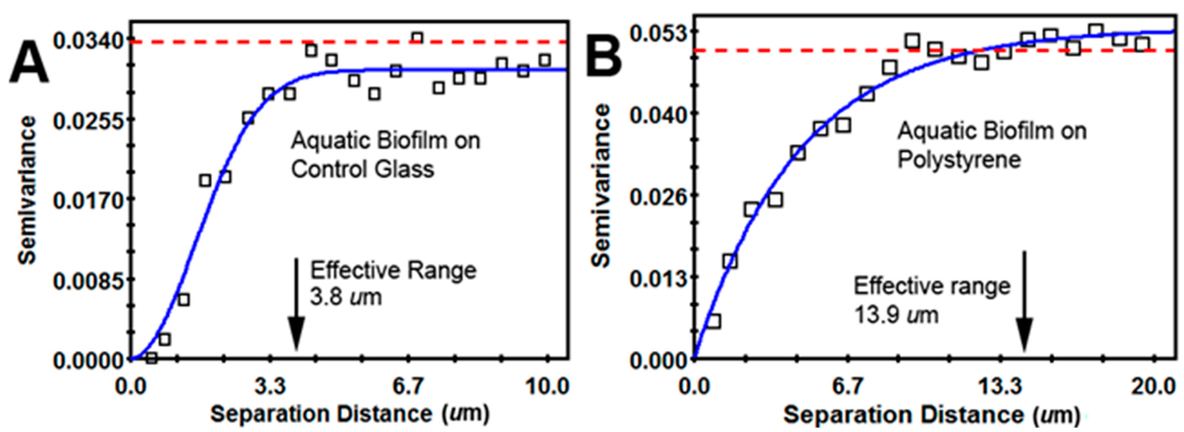
| Geostatistical Parameter | Plain Glass | Polystyrene | Interpretation |
|---|---|---|---|
| Residual ∑ Squares of the Best-Fit Model | 6.85 × 10⁻⁵ | 6.79 × 10⁻⁵ | Strong model fit to semivariance |
| Nugget Variance | 0.00001 | 0.00001 | Sufficient sampling at the proper spatial scale for both biofilm |
| Moran’s I Cluster Index Strength of Autocorrelation | +4.24 | +12.06 |  Polystyrene biofilm has 2.84-fold stronger autocorrelation Polystyrene biofilm has 2.84-fold stronger autocorrelation |
| Effective range of autocorrelated radial separation distances between cells (µm) | 3.8 | 13.9 | Polystyrene biofilm 3.66-fold wider radius of influence on clustered colonization behavior between neighboring cells |

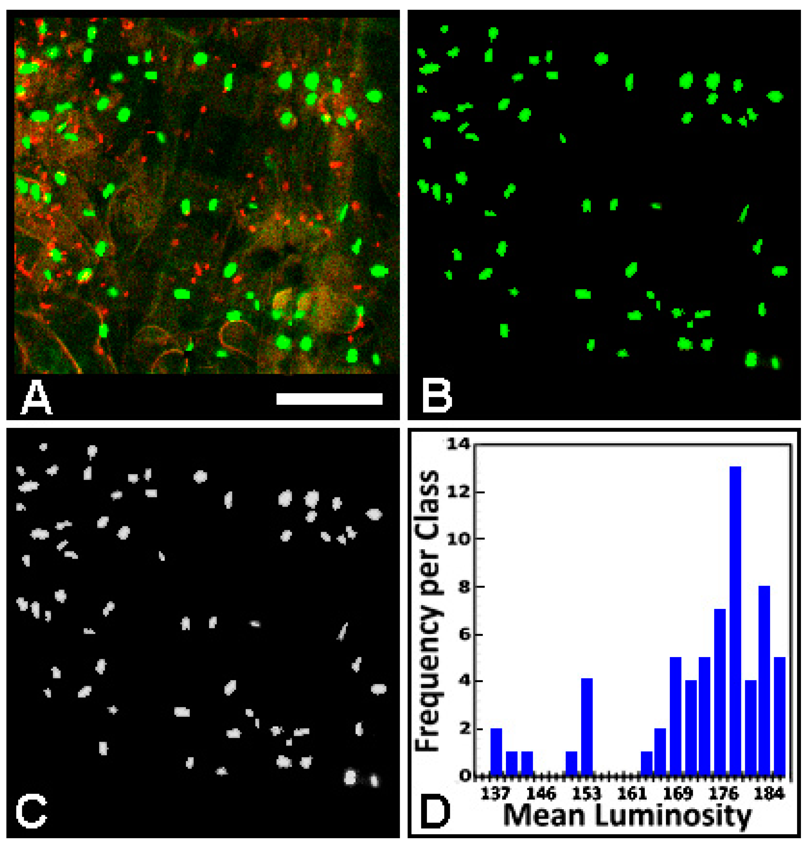
3.2.5. Color Segmentation Tool for Cell-Cell Communication/Gene Expression Studies
4. Summary and Concluding Statements
Acknowledgments
Author Contributions
Conflicts of Interest
References
- Liu, J.; Dazzo, F.B.; Glagoleva, O.; Yu, B.; Jain, A. CMEIAS: A computer-aided system for the image analysis of bacterial morphotypes in microbial communities. Microb. Ecol. 2001, 41, 173–194. [Google Scholar] [PubMed]
- Daims, H.; Lucker, S.; Wagner, M. Daime, a novel image analysis program for microbial ecology and biofilm research. Environ. Microbiol. 2006, 8, 200–213. [Google Scholar] [CrossRef] [PubMed]
- Daims, H.; Wagner, M. Quantification of uncultured microorganisms by fluorescence microscopy and digital image analysis. Appl. Microbiol. Biotechnol. 2007, 75, 237–248. [Google Scholar] [CrossRef] [PubMed]
- Dazzo, F.B.; Klemmer, K.J.; Chandler, R.; Yanni, Y. In situ ecophysiology of microbial biofilm communities analyzed by CMEIAS computer-assisted microscopy at single-cell resolution. Diversity 2013, 5, 426–460. [Google Scholar] [CrossRef]
- CMEIAS Center for Microbial Ecology Image Analysis System Project Website. Available online: http://cme.msu.edu/cmeias/ (accessed on 22 April 2013).
- Dazzo, F.B.; Mateos, P.; Orgambide, G.; Philip-Hollingsworth, S.; Squartini, A.; Subba-Rao, N.S.; Pankratz, H.S.; Baker, D.; Hollingsworth, R.; Whallon, J.; et al. The infection process in the Rhizobium-legume symbiosis and visualization of rhizoplane microorganisms by laser scanning confocal microscopy. In Trends in Microbial Ecology; Guerrero, R., Pedros-Alio, C., Eds.; Spanish Society for Microbiology: Barcelona, Spain, 1993; pp. 259–262. [Google Scholar]
- Schloter, M.; Borlinghaus, R.; Bode, W.; Hartmann, A. Direct identification and localization of Azospirillum in the rhizosphere of wheat using fluorescence-labeled monoclonal antibodies and confocal scanning laser microscopy. J. Microsc. 1993, 171, 173–177. [Google Scholar] [CrossRef]
- Assmus, B.; Hutzler, P.; Kirchhof, G.; Amann, R.; Lawrence, J.R.; Hartmann, A. In situ localization of Azospirillum brasilense in the rhizosphere of wheat with fluorescently labeled, rRNA-targeted oligonucleotide probes and scanning confocal laser microscopy. Appl. Environ. Microbiol. 1995, 61, 1013–1019. [Google Scholar] [PubMed]
- Chi, F.; Shen, S.H.; Cheng, H.P.; Jing, Y.X.; Yanni, Y.G.; Dazzo, F.B. Ascending migration of endophytic rhizobia, from roots to leaves, inside rice plants and assessment of benefits to rice growth physiology. Appl. Environ. Microbiol. 2005, 71, 7271–7278. [Google Scholar] [CrossRef] [PubMed]
- Lawrence, R.; Korber, D.R.; Neu, T.R. Analytical imaging and microscopy techniques. In Manual of Environmental Microbiology, 3rd ed.; Hurst, C.J., Crawford, R.L., Garland, J., Lipson, D., Mills, A., Stetzenback, L.J., Eds.; American Society for Microbiology Press: Washington, DC, USA, 2007; pp. 40–68. [Google Scholar]
- Lewandowski, Z.; Beyenal, H. Fundamentals of Biofilm Research; CRC: Boca Raton, FL, USA, 2007. [Google Scholar]
- Krambeck, C.; Krambeck, H.; Overbeck, J. Microcomputer assisted biomass determination of planktonic bacteria on scanning electron micrographs. Appl. Environ. Microbiol. 1981, 42, 142–149. [Google Scholar] [PubMed]
- Sieracki, M.; Viles, C. Enumeration and sizing of microorganisms using digital image analysis. In Digital Image Analysis of Microbes: Imaging, Morphometry, Fluorometry and Motility Techniques and Applications; Wilkinson, M.H.F., Schut, F., Eds.; Wiley: Chichester, UK, 1998; pp. 175–198. [Google Scholar]
- Sieracki, M.; Reichenbach, S.; Webb, K. Evaluation of automated threshold selection methods for accurately sizing microscopic fluorescent cells by image analysis. Appl. Environ. Microbiol. 1989, 55, 2762–2772. [Google Scholar] [PubMed]
- Folland, I.; Trione, D.; Dazzo, F.B. Accuracy of biovolume formulas for CMEIAS computer-assisted microscopy and body size analysis of morphologically diverse microbial populations and communities. Microb. Ecol. 2013, 68, 596–610. [Google Scholar] [CrossRef]
- Duda, R.; Hart, P. Pattern Classification and Scene Analysis; John Wiley & Sons: New York, NY, USA, 1973; pp. 103–132. [Google Scholar]
- Jain, A.K.; Zongker, D. Feature selection: Evaluation, application, and small sample performance. Inst. Electr. Electron. Eng. Trans. Pattern Anal. Mach. Intell. 1993, 19, 153–158. [Google Scholar]
- Rosin, P.; Venkatesh, S. Extracting natural scales using Fourier descriptors. Pattern Recognit. 1993, 26, 1383–1393. [Google Scholar] [CrossRef]
- Yu, B.; Yuan, B. A consistent attributed graph-based hand-drawn circuit diagram reading system. Chin. J. Electron. 1995, 4, 1–11. [Google Scholar]
- Robertson, G.P. Geostatistics in ecology: Interpolating with known variance. Ecology 1987, 68, 744–748. [Google Scholar] [CrossRef]
- Dazzo, F.B.; Joseph, A.R.; Gomaa, A.B.; Yanni, Y.G.; Robertson, G.P. Quantitative indices for the autecological biogeography of a Rhizobium endophyte of rice at macro and micro spatial scales. Symbiosis 2003, 35, 147–158. [Google Scholar]
- Dazzo, F.B. CMEIAS-aided microscopy of the spatial ecology of individual bacterial interactions involving cell-to-cell communication within biofilms. Sensors 2012, 12, 7047–7062. [Google Scholar] [CrossRef] [PubMed]
- Gross, C.A.; Reddy, C.; Dazzo, F.B. CMEIAS color segmentation: An improved computing technology to process color images for quantitative microbial ecology studies at single-cell resolution. Microb. Ecol. 2010, 59, 400–414. [Google Scholar] [CrossRef] [PubMed]
- Wiesmann, V.; Franz, D.; Held, C.; Munzenmayer, C.; Palmisano, R.; Wittenberg, T. Review of free software tools for image analysis of fluorescence cell micrographs. J. Microsc. 2014, 257. [Google Scholar] [CrossRef]
- Dazzo, F.B.; Liu, J.; Gross, C.; Reddy, C.; Monosmith, C.; Philips, N.; Radek, C.; Klemmer, K.J.; Ji, Z.; Smith, P.; et al. CMEIAS v3.10: Advanced computational tools of image analysis software designed to strengthen microscopy-based approaches for understanding microbial ecology. Proceedings of the 2013 All Scientists Meeting, Kellogg Biological Station Long-Term Ecological Research Program, Michigan State University, East Lansing, MI, USA; 2013. Available online: http://lter.kbs.msu.edu/abstracts/434 (accessed on 2 March 2015).
- Roberts, A.; Withers, P. StatistiXL, Version 1.10; Broadway-Nedlands: Kalamunda, Australia, 2012. [Google Scholar]
- Hammer, O.; Harper, D.A.T.; Ryan, P.D. PAST: Paleontological statistics software package for education and data analysis. Palaeontol. Electron. 2001, 4, 1–9. [Google Scholar]
- Towner, H. EcoStat, Version 1.03; Trinity Software Inc.: Campton, NH, USA, 1999. [Google Scholar]
- GS+, Version 7.0.; Gamma Design Software: Plainwell, MI, USA, 2004.
- Magurran, A.E. Measuring Biological Diversity; Blackwell Publishing: Malden, MA, USA, 2004. [Google Scholar]
- Hashsham, S.; Fernandez, A.; Dollhopf, S.; Dazzo, F.B.; Hickey, R.; Tiedje, J.M.; Criddle, C.S. Parallel processing of substrate correlates with greater functional stability in methanogenic bioreactor communities perturbed by glucose. Appl. Environ. Microbiol. 2000, 66, 4050–4057. [Google Scholar] [CrossRef] [PubMed]
- Fernandez, A.; Hashsham, S.; Dollhopf, D.; Raskin, L.; Glagoleva, O.; Dazzo, F.B.; Hickey, R.; Tiedje, J.M.; Criddle, C.S. Flexible community structure correlates with stable community function in methanogenic bioreactor communities perturbed by glucose. Appl. Environ. Microbiol. 2000, 66, 4058–4067. [Google Scholar] [CrossRef] [PubMed]
- Ritchie, M.E. Scale, Heterogeneity, and the Structure and Diversity of Ecological Communities; Princeton University Press: Princeton, NJ, USA, 2010. [Google Scholar]
- Yoshiyama, K.; Klausmeier, C.A. Optimal cell size for resource uptake in fluids: A new facet of resource competition. Am. Nat. 2008, 171, 59–70. [Google Scholar] [CrossRef] [PubMed]
- Lambshead, P.J.D.; Platt, H.M.; Shaw, K.M. The detection of differences among assemblages of marine benthic species based on an assessment of dominance and diversity. J. Nat. Hist. 1983, 17, 859–874. [Google Scholar] [CrossRef]
- Gaston, K.J. Rarity; Springer: Danvers, MA, USA, 1994. [Google Scholar]
- West, G.B.; Woodruff, W.H.; Brown, J.H. Allometric scaling of metabolic rate from molecules and mitochondria to cells and mammals. Proc. Natl. Acad. Sci. USA 2002, 99, 2473–2478. [Google Scholar] [CrossRef] [PubMed]
- Baker, R.M.; Singleton, F.L.; Hood, M.A. Effects of nutrient deprivation on Vibrio cholerae. Appl. Environ. Microbiol. 1983, 46, 930–940. [Google Scholar] [PubMed]
- Holmquist, L.; Kjelleberg, S. Changes in viability, respiratory activity, and morphology of the marine Vibrio sp. strain S14 during starvation of individual nutrients and subsequent recovery. FEMS Microbiol. Ecol. 1993, 12, 215–224. [Google Scholar] [CrossRef]
- Solow, A.R. A simple test for change in community structure. J. Anim. Ecol. 1993, 2, 191–193. [Google Scholar] [CrossRef]
- Tilman, D.; Knops, J.; Wedin, D.; Reich, P.; Ritchie, M.; Siemann, E. The influence of functional diversity and composition on ecosystem processes. Science 1997, 277, 1300–1302. [Google Scholar] [CrossRef]
- Shade, A.; Hogan, S.; Klimowicz, A.K.; Linske, M.; McManus, P.S.; Handelsman, J. Culturing captures members of the soil rare biosphere. Environ. Microbiol. 2012, 14, 2247–2252. [Google Scholar] [CrossRef] [PubMed]
- Schmitz, O. Predator diversity and trophic interactions. Ecology 2007, 88, 2415–2426. [Google Scholar] [CrossRef] [PubMed]
- Jürgens, K.; Arndt, H.; Zimmermann, H. Impact of metazoan and protozoan grazers on bacterial biomass distribution in microcosm experiments. Aquat. Microb. Ecol. 1997, 12, 131–138. [Google Scholar] [CrossRef]
- Hahn, M.W.; Moore, E.R.; Hofle, M.G. Bacterial filament formation, a defense mechanism against flagellate grazing, is growth rate controlled in bacteria of different phyla. Appl. Environ. Microbiol. 1999, 65, 25–35. [Google Scholar] [PubMed]
- Gonzalez, J.M.; Sherr, E.B.; Sherr, B.F. Size-selective grazing on bacteria by natural assemblages of estuarine flagellates and ciliates. Appl. Environ. Microbiol. 1990, 56, 583–589. [Google Scholar] [PubMed]
- Petchey, O.I.; Long, Z.T.; Morin, P.J. The consequences of body size in model microbial ecosystems. In Body Size: The Structure and Function of Aquatic Ecosystems; Hildrew, A., Raffelli, D., Edmonds-Brown, R., Eds.; Cambridge University Press: Cambridge, UK, 2007; pp. 245–265. [Google Scholar]
- Brown, J.H. Toward a metabolic theory of ecology. Ecology 2004, 45, 1771–1789. [Google Scholar] [CrossRef]
- Turner, M.G. Landscape ecology: The effect of pattern on process. Annu. Rev. Ecol. Syst. 1989, 20, 171–197. [Google Scholar] [CrossRef]
- Hassell, M.P.; May, R.M. Stability in insect host-parasite models. J. Anim. Ecol. 1973, 42, 693–726. [Google Scholar] [CrossRef]
- Perry, J. Measures of spatial patterns for counts. Ecology 1998, 79, 1008–1017. [Google Scholar] [CrossRef]
- Dazzo, F.B. CMEIAS digital microscopy and quantitative image analysis of microorganisms. In Microscopy: Science, Technology, Applications and Education; Microscopy Book Series #4; Mendez-Vilas, A., Diaz, J., Eds.; Formatex Res Center: Badajoz, Spain, 2010; pp. 1083–1090. [Google Scholar]
- Yanni, Y.G.; Rizk, R.Y.; Abd El-Fattah, F.K.; Squartini, A.; Corich, V.; Giacomini, A.; de Bruijn, F.; Rademaker, J.; Maya-Flores, J.; Ostrom, P.; et al. The beneficial plant growth-promoting association of Rhizobium leguminosarum bv. trifolii with rice roots. Aust. J. Plant Physiol. 2001, 28, 845–870. [Google Scholar]
- Dazzo, F.B. Applications of quantitative microscopy in studies of plant surface microbiology. In Plant Surface Microbiology; Varma, A., Abbott, L., Werner, D., Hampp, R., Eds.; Springer-Verlag: Berlin, Germany, 2004; pp. 503–550. [Google Scholar]
- Dazzo, F.B.; Schmid, M.; Hartmann, A. Immunofluorescence microscopy and fluorescence in situ hybridization combined with CMEIAS and other image analysis tools for soil- and plant-associated microbial autecology. In Manual of Environmental Microbiology, 3rd ed.; Garland, J., Hurst, C., Lipson, D., Mills, A., Stetzenbach, L., Crawford, R., Eds.; American Society for Microbiology Press: Washington, DC, USA, 2007; Chapter 59; pp. 712–733. [Google Scholar]
- Dazzo, F.B.; Yanni, Y.G. CMEIAS: An improved computing technology for quantitative image analysis of root colonization by rhizobacteria in situ at single-cell resolution. In Molecular Microbial Ecology of the Rhizosphere; DeBruijn, F., Ed.; John Wiley & Sons: New York, NY, USA, 2013; Volume 2, Chapter 69; pp. 733–742. [Google Scholar]
- Dazzo, F.B.; Gantner, S. Rhizosphere. In Topics in Ecological and Environmental Microbiology; Schmidt, T., Schaechter, M., Eds.; Elsevier Press: Waltham, MA, USA, 2012; pp. 467–479. [Google Scholar]
- Dazzo, F.B.; Ganesan, I.; Yanni, Y. Spatial ecology of rhizobacterial colonization on roots analyzed by CMEIAS computer-assisted microscopy at single-cell resolution. In Trends in Soil Ecology; Singh, D.P., Singh, H., Eds.; Studium Press: Houston, TX, USA, 2014; pp. 67–92. [Google Scholar]
- Fukuda, M.; Matsuyama, J.; Katano, T.; Nakano, S.; Dazzo, F.B. Assessing primary and bacterial production rates in biofilms on pebbles in Ishite Stream, Japan. Microb. Ecol. 2006, 52, 1–9. [Google Scholar] [CrossRef] [PubMed]
- Ji, Z.; Card, K.; Dazzo, F.B. CMEIAS JFrad: A new computing toolkit to discriminate the fractal geometry of landscape architecture and spatial patterns of individual cells in microbial biofilms. Microb. Ecol. 2014. [Google Scholar] [CrossRef]
- Dazzo, F.B.; Gross, C.A. CMEIAS Quadrat Maker: A digital software tool to optimize grid dimensions and produce quadrat images for landscape ecology spatial analysis. J. Ecosyst. Ecogr. 2013, 3, 1–4. [Google Scholar]
- Holgate, P. Some new tests of randomness. J. Ecol. 1965, 53, 261–266. [Google Scholar] [CrossRef]
- Ripley, B.D. Tests of “randomness” for spatial point patterns. J. R. Stat. Soc. 1979, 41, 368–374. [Google Scholar]
- Ettema, C.H.; Wardle, D.H. Spatial soil ecology. Trends Ecol. Evol. 2002, 17, 117–183. [Google Scholar] [CrossRef]
- Gantner, S.; Schmid, M.; Dürr, C.; Schuhegger, R.; Steidle, A.; Hutzler, P.R.; Langebartels, C.; Eberl, L.; Hartmann, A.; Dazzo, F.B.; et al. In situ spatial scale of calling distances and population density-independent N-acylhomoserine lactone mediated communication by rhizobacteria colonized on plant roots. FEMS Microb. Ecol. 2006, 56, 188–194. [Google Scholar] [CrossRef]
© 2015 by the authors; licensee MDPI, Basel, Switzerland. This article is an open access article distributed under the terms and conditions of the Creative Commons Attribution license (http://creativecommons.org/licenses/by/4.0/).
Share and Cite
Dazzo, F.B.; Niccum, B.C. Use of CMEIAS Image Analysis Software to Accurately Compute Attributes of Cell Size, Morphology, Spatial Aggregation and Color Segmentation that Signify in Situ Ecophysiological Adaptations in Microbial Biofilm Communities. Computation 2015, 3, 72-98. https://doi.org/10.3390/computation3010072
Dazzo FB, Niccum BC. Use of CMEIAS Image Analysis Software to Accurately Compute Attributes of Cell Size, Morphology, Spatial Aggregation and Color Segmentation that Signify in Situ Ecophysiological Adaptations in Microbial Biofilm Communities. Computation. 2015; 3(1):72-98. https://doi.org/10.3390/computation3010072
Chicago/Turabian StyleDazzo, Frank B., and Brighid C. Niccum. 2015. "Use of CMEIAS Image Analysis Software to Accurately Compute Attributes of Cell Size, Morphology, Spatial Aggregation and Color Segmentation that Signify in Situ Ecophysiological Adaptations in Microbial Biofilm Communities" Computation 3, no. 1: 72-98. https://doi.org/10.3390/computation3010072
APA StyleDazzo, F. B., & Niccum, B. C. (2015). Use of CMEIAS Image Analysis Software to Accurately Compute Attributes of Cell Size, Morphology, Spatial Aggregation and Color Segmentation that Signify in Situ Ecophysiological Adaptations in Microbial Biofilm Communities. Computation, 3(1), 72-98. https://doi.org/10.3390/computation3010072