Abstract
This research presents a comparative analysis of numerical methods for solving first-kind Fredholm integral equations using the Bubnov–Galerkin method with various wavelet and orthogonal polynomial bases. The bases considered are constructed from Legendre, Laguerre, Chebyshev, and Hermite wavelets, as well as Alpert multiwavelets and CAS wavelets. The effectiveness of these bases is evaluated by measuring errors relative to known analytical solutions at different discretization levels. Results show that global orthogonal systems—particularly the Chebyshev and Hermite—achieve the lowest error norms for smooth target functions. CAS wavelets, due to their localized and oscillatory nature, produce higher errors, though their accuracy improves with finer discretization. The analysis has been extended to incorporate perturbations in the form of additive noise, enabling a rigorous assessment of the method’s stability with respect to different wavelet bases. This approach provides insight into the robustness of the numerical scheme under data uncertainty and highlights the sensitivity of each basis to noise-induced errors.
1. Introduction
Fredholm integral equations of the first kind describe problems in which the observed data represent the integral effect of an unknown function. Such models arise naturally in applications where measurements capture an averaged or accumulated effect: in inverse heat conduction problems, tomographic reconstruction, spectroscopy, signal processing, and geophysical exploration, as well as in geochemical and gravimetric problems.
The main difficulty in solving these problems lies in their ill-posedness [1]. The ill-posed nature of such problems can be illustrated with a simple example: for a constant kernel and right-hand side, the integral equation reduces to recovering a function from its known integral (the area under its graph). This formulation admits infinitely many solutions since any family of functions with the same integral sum satisfies the condition, demonstrating a fundamental non-uniqueness of the solution without additional constraints [2,3].
Various methods are used to solve such problems by stabilizing them and incorporating prior information about the solution [4]. Among these are regularization methods, including the approaches of Tikhonov and Lavrentiev [5,6,7,8], spectral cutoff methods, and Bayesian approaches [9]. These techniques yield stable and physically meaningful solutions when recovering functions from integral data.
Effective methods for solving Fredholm integral equations also include numerical solution techniques and multilevel iterative schemes such as the Landweber method [10,11], the method of conjugate equations [12,13], projection methods [14], quadrature methods, collocation methods [15,16], and others [17,18].
Wavelet bases are widely used in projection-based numerical methods for solving Fredholm integral equations of the first kind. Their use is motivated by the ability to approximate functions locally and to represent operators in sparse form. Several studies consider specific types of polynomial and specialized wavelet bases.
In [19,20,21], a numerical method using Legendre wavelets for solving integral equations is proposed. The basic functions are constructed from Legendre polynomials, ensuring orthogonality on the standard interval and convenient decomposition of integral operators. The convergence of the approximate solution is also investigated.
Works [22,23] explore the use of Chebyshev wavelets as bases for solving Fredholm integral equations of the first kind. These bases are built from Chebyshev polynomials of the first kind and feature specific orthogonality properties and computational efficiency when decomposing the right-hand side and the kernel of the integral equation.
In [24], a method based on Hermite wavelets is studied for solving parabolic Volterra integro-differential equations. The basis is formed from Hermite polynomials and accounts for boundary conditions and the smoothness of the solution.
Reference [25] employs the Galerkin method with Laguerre wavelet bases for one-dimensional differential equations. The basic functions are defined via Laguerre polynomials and are applied to problems on unbounded intervals.
The classic work [26] introduces the concept of Alpert’s wavelet-like bases for accelerated solution of integral equations of the second kind, demonstrating the construction of sparse operator representations and the use of multilevel structure.
Reference [27] discusses the Petrov–Galerkin method with Alpert multiwavelet bases for solving second-kind nonlinear Fredholm integral equations.
References [28,29] consider a numerical method for solving integral and integro-differential equations based on approximating the unknown function with CAS wavelets (Cosine and Sine). The method represents the unknown function as a finite expansion in CAS wavelets, reducing the integral equation to a system of linear algebraic equations. The resulting system features a sparse coefficient matrix structure, facilitating its numerical solution.
The review in [30] summarizes known approaches, including the mentioned polynomial wavelet bases, and classifies the methods by the type of basis used and the numerical properties of the solution.
This study provides a review of wavelet bases and a comparative computational analysis of the approximate solution of Fredholm integral equations of the first kind using the Bubnov–Galerkin method with wavelet bases. The structure of the approximate solution based on the Bubnov–Galerkin method is presented, along with the construction techniques for the corresponding wavelet basis functions. The following wavelet bases are considered in this study: Legendre, Laguerre, Chebyshev, and Hermite wavelets, as well as Alpert multiwavelets and CAS wavelets. The results of numerical experiments are compared with polynomial bases and analytical solutions to identify more accurate approximate solutions. Computational experiments with additive noise were carried out for various wavelet types, followed by an analysis of the method’s stability with respect to noise, as well as a comparative evaluation of computational cost. The study highlights the most effective wavelet bases and analyzes the factors determining their accuracy and computational efficiency.
2. Materials and Methods
The general form of a Fredholm integral equation of the first kind is expressed as follows:
Here is the unknown function and is the known function, kernel is .
This equation is defined via a linear integral operator and is characterized by the fact that the unknown function appears under the integral sign. Thus, it is considered in the class of inverse problems.
2.1. Bubnov–Galerkin Method
To approximate this equation, the solution can be represented using special basis functions as follows:
where is an orthonormal system consisting of wavelets, and are the unknown coefficients.
Substituting this expression into the original equation and using the linearity property, it can be rewritten in the following form:
According to the Bubnov–Galerkin method, we apply the orthogonality conditions by taking the inner product of both sides of the equation with the basic functions, as follows:
where and .
To transform the resulting system from a four-index structure into a two-dimensional matrix form, we renumber the indices according to the following rule:
As a result, we obtain a system of linear algebraic equations for the unknown coefficients. The problem described above is thus reduced to solving the following system:
Matrix form is presented as follows:
where
and the elements of the matrix and vector are defined as follows:
2.2. Alpert Wavelets
Alpert wavelets are constructed using polynomial functions and include several orthonormal functions at each scaling level. They are used for highly accurate local representation of signals and are closely related to the theory of polynomial approximation [26,27].
Alpert wavelets are defined through scaling functions , which are derived from the first Legendre polynomials restricted to the interval , followed by shifting and scaling. These functions have the following properties:
- They are defined on the interval .
- They form an orthonormal set
- These functions generate the space of polynomials up to degree .
For each scaling function, a corresponding set of basic wavelets is defined. These functions are also orthonormal and are divided into two parts (for example, and ), on each of which they are defined polynomially:
where and are polynomials indexed by .
Alpert wavelets are defined as follows:
where is the scaling level and is the shift parameter. These functions form a basis of wavelet functions on each of the subintervals partitioning the interval .
These functions form a basis of wavelet functions on each of the subintervals of .
2.2.1. Alpert Wavelet Function Spaces
For integer and the space of piecewise-polynomial functions is defined as follows:
where is the space of polynomials of degree less than . The dimension of this space is as follows:
and there exists an inclusion relationship between the spaces, as follows:
For each , we define the space as the orthogonal complement of in :
and then, by induction, we obtain the following decomposition:
2.2.2. Definition of Functions
Let be a set of functions forming an orthonormal basis for . Since is orthogonal to , the functions annihilate the first moments
To construct , first define functions on with the following properties:
- is a polynomial of degree at most on ;
- on the interval it is continued as an even or odd function depending on the parity of ;
- wavelets satisfy orthonormality
- wavelets satisfy the moment annihilation conditions
Verification of these properties for is performed directly. Then the functions are defined by the following equation:
and
In general form it will be presented as follows:
2.3. Chebyshev Wavelets
Chebyshev wavelets have the form with four arguments: , is any positive integer, is the degree of the Chebyshev polynomial of the second kind, and is the normalized time [31].
On the interval , Chebyshev wavelets are defined as follows:
where
and , , is any positive integer.
Here are Chebyshev polynomials of order , which are orthogonal on with the weight function
They are computed using the recursive formula as in [32]:
2.4. Hermite Wavelets
Hermite wavelets are defined as in [33,34]:
where
and , , is any positive integer.
Here, denotes the Hermite polynomials of degree , defined on the real line with respect to the weight function . They satisfy the following recurrence:
2.5. Laguerre Wavelets
On the interval Laguerre wavelets are given in the form as in [35]:
Here , and are any positive integers, is the degree of the Laguerre polynomial, and is the normalized time.
Here are Laguerre polynomials, orthogonal on with the weight function . Polynomials are defined by the recurrence formula:
2.6. Legendre Wavelets
For the approximate representation of the solution, Legendre wavelets of the form are used. These functions are defined as in [19]:
where , , , and are positive numbers.
Legendre polynomials are orthogonal with respect to the weight function on the interval and defined by the recurrence relation as follows:
These polynomials form a complete orthonormal basis in the space . Moreover, they are uniformly bounded.
2.7. CAS Wavelets
CAS wavelets have four arguments where , can assume any nonnegative integer, is any integer, and is the normalized time. They are defined on the interval as in [28,29]:
where .
3. Results and Discussion
3.1. Computational Experiment for Test Problem 1
Consider the Fredholm integral equation of the following form:
The exact analytical solution is known:
The table below shows the values of the absolute error between the analytical (exact) solution and the approximate solutions obtained using polynomial basis and different wavelet bases as in Table 1: Alpert, Chebyshev, Legendre, Hermite, CAS and Laguerre at the nodal points in the interval .

Table 1.
Representation of different wavelets: Alpert, Chebyshev, Hermite, Laguerre, Legendre, and CAS for the cases and .
In this case, a numerical analysis was carried out for various basis systems for parameters and (Table 2 and Table 3, respectively). The errors of the approximate solutions were evaluated on a uniform grid over the interval and norms were computed.
Table 2.
Table of errors of solving first-kind Fredholm integral equation using Bubnov–Galerkin method with wavelet-basis for first problem in the case when and .
Table 3.
Table of errors of solving first-kind Fredholm integral equation using Bubnov–Galerkin method with wavelet-basis for first problem in the case when and .
The discrete norm of the error between the exact solution and the approximate solution is given by the following equation:
where are quadrature nodes on , and are the corresponding quadrature weights.
For the case , , the computed norms were Alpert—, Chebyshev—, Hermite—, Laguerre—, Legendre—, CAS—, Polynomial basis—.
For , , the corresponding values were Alpert—, Chebyshev—, Hermite—, Laguerre—, Legendre—, CAS—, Polynomial basis—.
Analysis of these results shows that the smallest error norms at both parameter levels are achieved using the global orthogonal systems Chebyshev, Hermite, and polynomial basis in the form of a power function. These bases exhibit the best alignment with the nature of the analytical solution , which is smooth over the interval.
As the number of intervals increases, the approximation of the solution using the CAS wavelet basis becomes more accurate (Figure 1a–d). This relationship can be expressed as follows:
where is any nonnegative integer, it denotes the vector of CAS wavelet basis functions evaluated at , and is the vector of the corresponding expansion coefficients. The limit signifies that as tends to infinity, the sum of wavelet terms more precisely reconstructs the target function , ensuring convergence to the true solution over the domain.
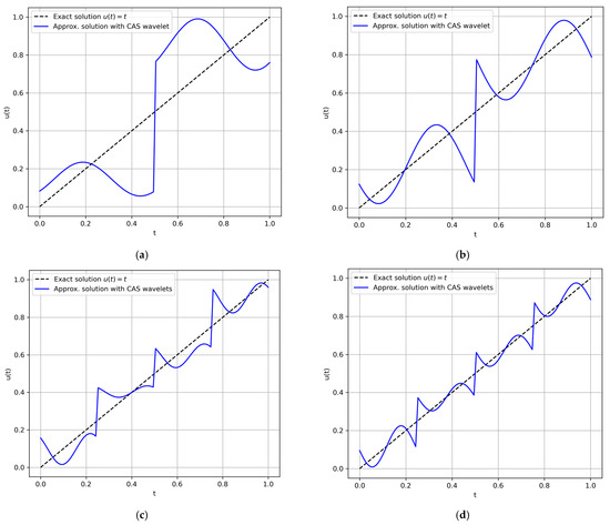
Figure 1.
Plots comparing the exact solution and the approximate solution obtained using CAS wavelets for the following cases: (a) ; (b) ; (c) ; and (d) .
3.2. Computational Experiment for Test Problem 2
Consider the Fredholm integral equation of the following form:
The exact analytical solution is known and is as follows:
The table below shows the values of the absolute error between the analytical (exact) solution and the approximate solutions obtained using different wavelet bases: Alpert, Chebyshev, Legendre, Hermite, CAS and Laguerre at the nodal points in the interval .
For , the resulting error norms were as follows (Table 4): Alpert—, Chebyshev—, Hermite—, Laguerre—, Legendre—, CAS—, Polynomial basis—. The Hermite basis showed the best performance, with errors considerably lower than those of the other systems. For , there was a significant reduction in errors for all global orthogonal bases (Table 5): Alpert—5, Chebyshev—5, Hermite—5, Laguerre—5, Legendre—5, whereas the CAS basis remained at the level of and the Polynomial basis yielded an error of approximately .
Table 4.
Table of errors of solving the first-kind Fredholm integral equation using the Bubnov–Galerkin method with wavelet basis for the second problem in the case when and .
Table 5.
Table of errors of solving the first-kind Fredholm integral equation using the Bubnov–Galerkin method with wavelet basis for second problem in the case when and .
For , there was a significant reduction in errors for all global orthogonal bases (Table 6): Alpert—3, Chebyshev—3, Hermite—3, Laguerre—9, Legendre—3, whereas the CAS basis remained at the level of and the Polynomial basis yielded an error of approximately .
Table 6.
Table of errors of solving the first-kind Fredholm integral equation using the Bubnov–Galerkin method with wavelet basis for the second problem in the case when and .
These results demonstrate the high effectiveness of global orthogonal systems in approximating smooth exponential solutions such as , especially as the discretization parameter increases.
The presented Figure 2a–g show the plots of basic functions used in the Bubnov–Galerkin method for solving integral equations: the Alpert, Chebyshev, Hermite, Laguerre, Legendre wavelets, and the polynomial basis illustrate various global orthogonal systems characterized by smooth functional forms, while the CAS wavelets exhibit a more oscillatory structure, highlighting differences in the degree of localization, number of oscillations, and their ability to approximate local features of the solution.
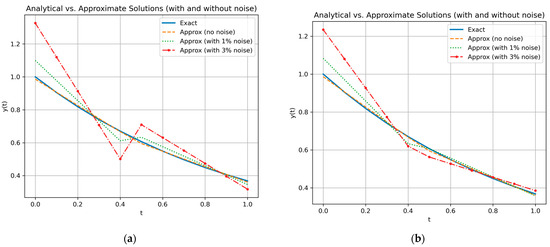
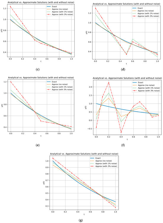
Figure 2.
Plots of the exact solution and the approximate solution using wavelets (): (a) Alpert; (b) Chebyshev; (c) Hermite; (d) Laguerre; (e) Legendre; (f) CAS wavelet; (g) Polynomial basis.
To assess the influence of noise on the accuracy of numerical solutions to the first-kind Fredholm integral equation using the Bubnov–Galerkin method, there was analyzed the variation in absolute error when the noise level in the right-hand side increases from 1% to 3% (Figure 2a–g and Figure 3a–f). The following wavelet bases were considered: Alpert, Chebyshev, Hermite, Laguerre, and Legendre wavelets.
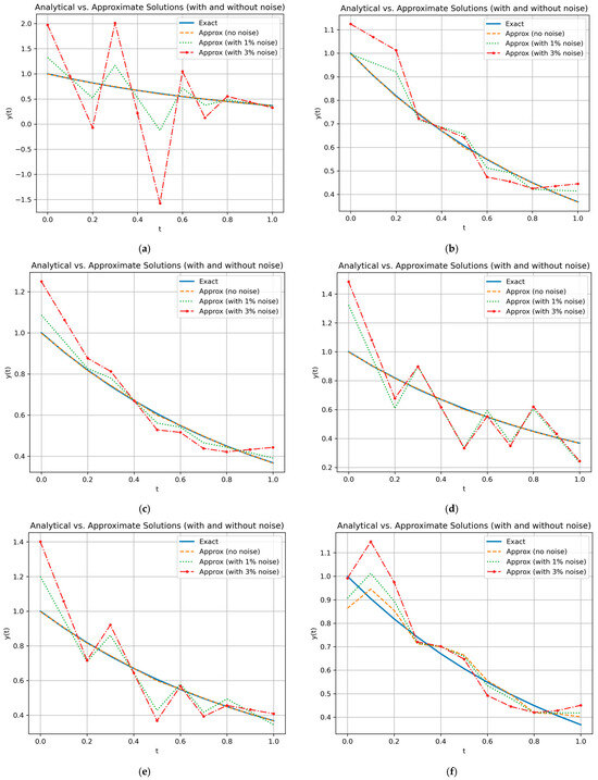
Figure 3.
Plots of the exact solution and the approximate solution using wavelets (): (a) Alpert; (b) Chebyshev; (c) Hermite; (d) Laguerre; (e) Legendre; (f) CAS wavelet.
The table below presents the mean absolute errors at each noise level, along with the corresponding increase and multiplicative growth.
The Chebyshev and Hermite wavelets yield the lowest mean absolute errors for both 1% and 3% noise levels. The error increases from 0.024472 to 0.064613 (a 2.64-fold growth), indicating high accuracy and good stability against additive noise.
The Legendre wavelets demonstrate comparable accuracy at 1% noise (0.025568), but slightly larger error growth at 3% (to 0.072027), which corresponds to a 2.82-fold increase.
The Alpert wavelets show relatively higher errors at both noise levels, with a substantial increase (2.89-fold), suggesting lower robustness under noisy conditions.
The Laguerre wavelets exhibit minimal error growth (only 1.08 times) as noise increases. However, the absolute error remains significantly larger than with other bases, indicating low sensitivity to noise but also low approximation accuracy, even for mild noise levels (Table 7).
Table 7.
Error increase in wavelet approximations under 1% and 3% noise.
Numerical experiments with CAS wavelets revealed pronounced oscillations in the approximate solution. This behavior is primarily attributed to the lack of orthonormality of the basic functions, as well as the presence of trigonometric components in their structure. Unlike polynomial-based wavelets, the use of sinusoidal functions without proper orthogonality leads to the amplification of spurious oscillations and instability in the approximation. As a result, the CAS basis is less suitable for the stable numerical solution of first-kind Fredholm integral equations, particularly in the presence of noise.
Among the wavelet bases, the Laguerre wavelet demonstrated the best performance in terms of computation time (0.0769 s), ensuring the lowest resource consumption among the compared wavelets (Table 8). The highest computation time was observed for the CAS wavelets (0.2793 s).
Table 8.
Computation time for different bases and .
Numerical experiments demonstrate that increasing the number of intervals—equivalent to expanding the wavelet basis space in the Bubnov–Galerkin method—does not lead to a significant change in the mean error of the approximate solution in the presence of noise in the right-hand side of the first-kind Fredholm integral equation. An important observation is that, regardless of the noise level (1% or 3%), the error exhibits a similar pattern of growth when transitioning to a more refined decomposition, indicating the method’s robustness with respect to noise under an increased number of basic functions.
The obtained results suggest that expanding the basis does not compromise the numerical stability of the method and does not increase the sensitivity of the approximate solution to fluctuations in the input data. Thus, the increase in the number of intervals preserves the balance between accuracy and stability, confirming the validity of the constructed approximation space and the appropriateness of the chosen wavelet bases. However, the absence of a reduction in the mean error indicates the need for additional stabilization techniques in order to achieve higher accuracy under noisy conditions.
4. Conclusions
This study provided a comprehensive review and computational analysis of solving first-kind Fredholm integral equations using the Bubnov–Galerkin method with a variety of wavelet and orthogonal polynomial bases. The considered bases included functions derived from Legendre, Laguerre, Chebyshev, and Hermite polynomials, as well as Alpert multiwavelets and CAS wavelets.
Numerical experiments were carried out for parameter configurations with and , evaluating the accuracy of approximate solutions against known analytical solutions using the norm. The results demonstrate that global orthogonal bases—particularly Chebyshev, Hermite, and the polynomial basis—consistently achieved the lowest error norms. For instance, with , these bases showed significantly reduced errors. In contrast, the CAS wavelet basis, due to its localized and oscillatory nature, produced notably higher error norms; however, its performance improved with an increased discretization parameter , enabling more accurate approximation of the target solution.
In addition, experiments with additive noise were conducted to assess the robustness of each basis. The analysis revealed that global bases such as Chebyshev and Hermite maintained high accuracy and demonstrated superior stability under noisy conditions. Conversely, localized wavelets like CAS exhibited greater sensitivity to perturbations but showed gradual improvement with finer resolution.
These findings highlight the importance of selecting a basis that aligns with the smoothness, global behavior, and noise sensitivity of the underlying solution. In particular, the Hermite and Chebyshev bases proved especially effective for approximating both polynomial and exponential-type functions in smooth settings.
Overall, the results indicate that global orthogonal bases offer a reliable and accurate framework for solving first-kind Fredholm integral equations, especially in the presence of noise, where stability and approximation quality are essential.
Author Contributions
Conceptualization, supervision, project administration, N.T.; software, validation, writing—review and editing, A.T.; formal analysis, data curation, visualization, T.M.; methodology, investigation, writing—original draft preparation, writing—review and editing, D.T. All authors have read and agreed to the published version of the manuscript.
Funding
The research is funded by Science Committee of the Ministry of Science and Higher Education of the Republic of Kazakhstan (Grant No. BR27100483 “Development of predictive exploration technologies for identifying ore-prospective areas based on data analysis from the unified subsurface user platform “Minerals.gov.kz” using artificial intelligence and remote sensing methods”).
Data Availability Statement
The authors declare that the data supporting the findings of this study are available within the paper. Additional data and clarifications can be provided on request from the corresponding author.
Conflicts of Interest
The authors declare no conflicts of interest.
References
- Kabanikhin, S.I.; Shishlenin, M.A. Theory and Numerical Methods for Solving Inverse and Ill-Posed Problems. J. Inverse Ill-Posed Probl. 2019, 27, 453–456. [Google Scholar] [CrossRef]
- Bitsadze, A.V. Integral Equations of First Kind, 1st ed.; World Scientific: Singapore, 1995; Volume 7. [Google Scholar]
- Krisch, A. An Introduction to the Mathematical Theory of Inverse Problems, 1st ed.; Springer: New York, NY, USA, 1996; pp. 1–300. [Google Scholar] [CrossRef]
- Baker, C.T.H. The Numerical Treatment of Integral Equations, 1st ed.; Clarendon Press: Oxford, UK, 1977; pp. 1–250. [Google Scholar]
- Tikhonov, A.N.; Goncharsky, A.V.; Stepanov, V.V.; Yagola, A.G. Numerical Methods for the Solution of Ill-Posed Problems, 1st ed.; Kluwer Academic Publishers: Dordrecht, The Netherlands, 1995; pp. 1–350. [Google Scholar] [CrossRef]
- Weese, J. A Reliable and Fast Method for the Solution of Fredholm Integral Equations of the First Kind Based on Tikhonov Regularization. Comput. Phys. Commun. 1992, 69, 99–111. [Google Scholar] [CrossRef]
- Kabanikhin, S.I.; Shishlenin, M.A.; Nurseitov, D.B.; Nurseitova, A.T.; Kasenov, S.E. Comparative Analysis of Methods for Regularizing an Initial Boundary Value Problem for the Helmholtz Equation. J. Appl. Math. 2014, 2014, 786326. [Google Scholar] [CrossRef]
- Altürk, A.; Cosgun, T. The Use of Lavrentiev Regularization Method in Fredholm Integral Equations of the First Kind. Int. J. Adv. Appl. Math. Mech. 2019, 7, 70–79. [Google Scholar]
- Hanson, R.J. A Numerical Method for Solving Fredholm Integral Equations of the First Kind Using Singular Values. SIAM J. Numer. Anal. 1971, 8, 616–622. [Google Scholar] [CrossRef]
- Luo, X.; Hu, W.; Xiong, L.; Li, F. Multilevel Jacobi and Gauss–Seidel Type Iteration Methods for Solving Ill-Posed Integral Equations. J. Inverse Ill-Posed Probl. 2015, 23, 477–490. [Google Scholar] [CrossRef]
- Landweber, L. An Iteration Formula for Fredholm Integral Equations of the First Kind. Am. J. Math. 1951, 73, 615–624. [Google Scholar] [CrossRef]
- Marchuk, G.I. Conjugate Equations: A Course of Lectures, 1st ed.; IVM RAS: Moscow, Russia, 2000; p. 335. (In Russian) [Google Scholar]
- Temirbekov, N.; Temirbekova, L. Using the Conjugate Equations Method for Solving Inverse Problems of Mathematical Geophysics and Mathematical Epidemiology. AIP Conf. Proc. 2021, 2325, 020023. [Google Scholar] [CrossRef]
- Temirbekov, N.M.; Temirbekova, L.N.; Nurmangaliyeva, M.B. Numerical Solution of the First Kind Fredholm Integral Equations by Projection Methods with Wavelets as Basis Functions. TWMS J. Pure Appl. Math. 2022, 13, 105–118. [Google Scholar] [CrossRef]
- Atkinson, K.E. The Numerical Solution of Integral Equations of the Second Kind, 1st ed.; Cambridge University Press: Cambridge, UK, 1997; pp. 1–300. [Google Scholar] [CrossRef]
- Maleknejad, K.; Aghazadeh, N.; Mollapourasl, R. Numerical Solution of Fredholm Integral Equation of the First Kind with Collocation Method and Estimation of Error Bound. Appl. Math. Comput. 2006, 179, 352–359. [Google Scholar] [CrossRef]
- Polozhiy, G.N. On a Method for Solving Integral Equations. Izv. USSR Acad. Sci. Ser. Math. 1959, 23, 295–312. [Google Scholar]
- Twomey, S. On the Numerical Solution of Fredholm Integral Equations of the First Kind by the Inversion of the Linear System Produced by Quadrature. J. ACM 1963, 10, 97–101. [Google Scholar] [CrossRef]
- Maleknejad, K.; Sohrabi, S. Numerical Solution of Fredholm Integral Equations of the First Kind by Using Legendre Wavelets. Appl. Math. Comput. 2007, 186, 836–843. [Google Scholar] [CrossRef]
- Tamabay, D.; Temirbekov, N.; Zhumagulov, B. Approximate Solution of Nonlinear Integral Hammerstein Equations by Projection Method Using Multiwavelets. AIP Conf. Proc. 2023, 2879, 040012. [Google Scholar] [CrossRef]
- Shang, X.; Han, D. Numerical Solution of Fredholm Integral Equations of the First Kind by Using Linear Legendre Multi-Wavelets. Appl. Math. Comput. 2007, 191, 440–444. [Google Scholar] [CrossRef]
- Bahmanpour, M.; Fariborzi Araghi, M.A. A Method for Solving Fredholm Integral Equations of the First Kind Based on Chebyshev Wavelets. Anal. Theory Appl. 2013, 29, 197–207. [Google Scholar] [CrossRef]
- Adibi, H.; Assari, P. Chebyshev Wavelet Method for Numerical Solution of Fredholm Integral Equations of the First Kind. Math. Probl. Eng. 2010, 2010, 138408. [Google Scholar] [CrossRef]
- Turan Dincel, A.; Tural Polat, S.N.; Sahin, P. Hermite Wavelet Method for Nonlinear Fractional Differential Equations. Fractal Fract. 2023, 7, 346. [Google Scholar] [CrossRef]
- Shiralashetti, S.C.; Angadi, L.M.; Kumbinarasaiah, S. Laguerre Wavelet-Galerkin Method for the Numerical Solution of One Dimensional Partial Differential Equations. RN 2018, 55, 7. [Google Scholar]
- Alpert, B.K. A class of bases in L2 for the sparse representation of integral. SIAM J. Sci. Comput. 1993, 14, 159–184. [Google Scholar] [CrossRef]
- Maleknejad, K.; Karami, M. Numerical Solution of Non-Linear Fredholm Integral Equations by Using Multiwavelets in the Petrov–Galerkin Method. Appl. Math. Comput. 2005, 168, 102–110. [Google Scholar] [CrossRef]
- Yousefi, S.; Banifatemi, A. Numerical Solution of Fredholm Integral Equations by Using CAS Wavelets. Appl. Math. Comput. 2006, 183, 458–463. [Google Scholar] [CrossRef]
- Saeedi, H.; Moghadam, M.M. Numerical Solution of Nonlinear Volterra Integro-Differential Equations of Arbitrary Order by CAS Wavelets. Commun. Nonlinear Sci. Numer. Simul. 2011, 16, 1216–1226. [Google Scholar] [CrossRef]
- Yuan, D.; Zhang, X. An Overview of Numerical Methods for the First Kind Fredholm Integral Equation. SN Appl. Sci. 2019, 1, 1178. [Google Scholar] [CrossRef]
- Zhou, F.; Xu, X. Numerical Solution of the Convection Diffusion Equations by the Second Kind Chebyshev Wavelets. Appl. Math. Comput. 2014, 247, 353–367. [Google Scholar] [CrossRef]
- Ghasemi, M.; Kajani, M.T. Numerical Solution of Time-Varying Delay Systems by Chebyshev Wavelets. Appl. Math. Model. 2011, 35, 5235–5244. [Google Scholar] [CrossRef]
- Kumar, S.; Ghosh, S.; Kumar, R.; Jleli, M. A Fractional Model for Population Dynamics of Two Interacting Species by Using Spectral and Hermite Wavelets Methods. Numer. Methods Partial Differ. Equ. 2021, 37, 1652–1672. [Google Scholar] [CrossRef]
- Saeed, U.; ur Rehman, M. Hermite Wavelet Method for Fractional Delay Differential Equations. J. Differ. Equ. 2014, 2014, 359093. [Google Scholar] [CrossRef]
- Zhou, F.; Xu, X. Numerical Solutions for the Linear and Nonlinear Singular Boundary Value Problems Using Laguerre Wavelets. Alderremy, A.A.; Shah, R.; Shah, N.A.; Aly, S.; Nonlaopon, K. Evaluation of Fractional-Order Pantograph Delay Differential Equation via Modified Laguerre Wavelet Method. Symmetry 2022, 14, 2356. [Google Scholar] [CrossRef]


Disclaimer/Publisher’s Note: The statements, opinions and data contained in all publications are solely those of the individual author(s) and contributor(s) and not of MDPI and/or the editor(s). MDPI and/or the editor(s) disclaim responsibility for any injury to people or property resulting from any ideas, methods, instructions or products referred to in the content. |
© 2025 by the authors. Licensee MDPI, Basel, Switzerland. This article is an open access article distributed under the terms and conditions of the Creative Commons Attribution (CC BY) license (https://creativecommons.org/licenses/by/4.0/).