Abstract
This study investigates optimal intervention strategies for controlling the spread of two co-circulating strains of SARS-CoV-2 within the Nigerian population. A newly formulated epidemiological model captures the transmission dynamics of the dual-strain system and incorporates three key control mechanisms: vaccination, non-pharmaceutical interventions (NPIs), and therapeutic treatment. To identify the most effective approach, Pontryagin’s Maximum Principle is employed, enabling the derivation of an optimal control function that minimizes both infection rates and associated implementation costs. Through numerical simulations, this study evaluates the performance of individual, paired, and combined intervention strategies. Additionally, a cost-effectiveness assessment based on the Incremental Cost-Effectiveness Ratio (ICER) framework highlights the most economically viable option, while results suggest that the combined application of vaccination and treatment strategies offers superior control over dual-strain transmission and implementing all three strategies together ensures the most robust suppression of the outbreak.
1. Introduction
Optimal Control Theory (OCT) is a foundational area of mathematical optimization that seeks to determine control strategies for dynamic systems in order to achieve specific objectives—often minimizing cost or maximizing system efficiency. Its origins trace back to the early 1950s, evolving from the calculus of variations, which focused on optimizing functionals over time. A major breakthrough was the introduction of Pontryagin’s Maximum Principle by Lev Pontryagin in 1956, providing necessary conditions for optimality analogous to the Euler–Lagrange equations in variational calculus. Around the same period, Richard Bellman’s development of dynamic programming laid the foundation for the Hamilton–Jacobi–Bellman (HJB) equation, a pivotal tool in solving optimal control problems [1,2,3]. During the 1970s and 1980s, OCT expanded significantly across various disciplines, including economics, engineering, and the life sciences, supported by advances in numerical methods. The theory has since grown to address stochastic systems influenced by randomness and robust systems characterized by uncertainty. In epidemiology, OCT plays a vital role in the formulation of adaptive strategies to mitigate infectious disease outbreaks. It incorporates parameters such as intervention cost, transmission rate, and limited healthcare resources to determine time-dependent policies that optimize both health outcomes and cost-efficiency [4].
COVID-19, a novel infectious disease caused by the SARS-CoV-2 virus, was first reported in Wuhan, China, in December 2019. Its rapid international spread prompted the World Health Organization (WHO) to declare it a global pandemic in March 2020. Since then, COVID-19 has caused substantial global morbidity and mortality, especially among the elderly and individuals with pre-existing health conditions [5,6]. Transmission primarily occurs via respiratory droplets, with symptom severity ranging from mild to critical and asymptomatic cases contributing to silent spread. Global control efforts have relied on public health interventions such as social distancing, mask usage, hand hygiene, and vaccination [6,7]. Beyond its health burden, the pandemic has led to profound socioeconomic disruptions, highlighting weaknesses in healthcare systems and the need for coordinated international responses.
The virus has continuously evolved, producing numerous variants with varying transmissibility, virulence, and immune escape potential. Among these, Alpha (B.1.1.7) emerged in the UK, Beta (B.1.351) in South Africa, Gamma (P.1) in Brazil, Delta (B.1.617.2) in India, and Omicron (B.1.1.529) globally in late 2021 [8,9,10,11,12,13,14]. Omicron’s mutations particularly in the spike protein raised concerns regarding reduced vaccine efficacy and increased spread of the disease, Authors in [15,16] formulated a mathematical model to examine COVID-19 transmission dynamics, incorporating vaccination, while Omorogie et. al. include treatment. Their results show that high vaccination and treatment rates, along with reduced vaccine inefficacy, can eliminate the virus [16].
In Nigeria, the prevailing SARS-CoV-2 variants have mirrored global patterns. Eta and Alpha were initially dominant, followed by Delta in 2021 and, more recently, Omicron and its sub-lineages. Genomic surveillance by Nigerian health authorities has been crucial in tracking these changes and guiding policy [5,10]. However, numerous studies, such as [17,18,19,20,21,22,23], have applied OCT in epidemiological contexts. For instance, Yusuf et al. [18] developed a deterministic model for tuberculosis (TB) transmission that incorporates three time-dependent controls—vaccination, treatment for drug-sensitive TB, and treatment for drug-resistant TB. Using Pontryagin’s Maximum Principle, they derived optimality conditions and conducted numerical simulations to assess the relative effectiveness and cost efficiency of individual and combined strategies. Their results suggested that while simultaneous application of all controls was most effective, resource-limited contexts could prioritize vaccination and drug-sensitive treatment. In a non-epidemiological application, Seun et al. [19] applied OCT to model criminal gang dynamics, with time-dependent controls targeting prevention and detection. They evaluated optimal strategies using the Runge–Kutta fourth-order method, along with cost-effectiveness analysis. Akinyemi et al. [20] formulated a model for Mpox that included human-to-animal and animal-to-human transmission, calibrating it with data from Nigeria and Germany. Their study incorporated optimal control and cost-effectiveness analysis and concluded that strategies promoting hygiene and behavioral change were the most effective interventions. Zakary et al. [21] analyzed Ebola dynamics across multiple regions, using a model including awareness campaigns, treatment, and travel restrictions. They applied Pontryagin’s principle and forward–backward sweep methods, concluding that combining public awareness and movement restrictions could effectively reduce transmission. Similarly, De la Sen et al. [22] developed an extended the SEIADR model for Ebola, integrating control strategies like vaccination and corpse disposal, and evaluated intervention effectiveness through numerical simulations. Laarabi et al. [23] focused on an SIR model with a saturated incidence rate and derived optimal vaccination strategies to minimize infections and increase recovery.
While substantial research has been conducted on COVID-19 using OCT, most models consider a single viral strain. However, the presence of multiple co-circulating strains has introduced new complexities that require more comprehensive modeling approaches [24,25,26,27,28,29]. For instance, Yusuf et al. [24] approached the pandemic as a multi-control problem involving personal protection, testing, treatment, and contact tracing. Using the forward–backward sweep method and the Runge–Kutta scheme, they demonstrated that combined interventions substantially reduced transmission in a cost-effective manner. Kouidere et al. [25] proposed a five-compartment model addressing awareness, diagnostics, and quarantine, with optimal control strategies including airport screening and public education. Zhong et al. [26] developed and analyzed a model with and without vaccination. They later introduced four control strategies—prevention, vaccination, rapid screening, and case identification—and demonstrated their effectiveness through numerical simulations. Manotosh et al. [30] incorporated media-based awareness and quarantine into a COVID-19 model, evaluating optimal controls for minimizing infections and implementation costs. Their simulations supported adaptive strategies for effective outbreak response. Models that consider dual or multiple strains provide a more realistic framework for evaluating disease dynamics. For example, Khajji et al. [31] modeled two COVID-19 strains and used Pontryagin’s principle to identify optimal strategies involving vaccination and awareness. Their results showed a marked reduction in infections and increased quarantining when controls were implemented. Elqaddaoui et al. [32] proposed a discrete time model tracking variant spread with targeted vaccination and treatment strategies for each strain. They applied Pontryagin’s principle and solved the optimality system iteratively, confirming the efficacy of their approach through numerical experiments.
Motivated by the need for multiple-strain COVID-19 models and an effective intervention design, this study builds on existing dual-strain frameworks. The objective is to identify optimal combinations of vaccination, treatment, and non-pharmaceutical interventions that minimize disease burden and implementation costs in a resource-limited setting like Nigeria. The contributions of this study include the following:
- i
- The development of an epidemic model that accounts for the dual-strain characteristics of COVID-19, evaluating the impact of various control strategies;
- ii
- Investigation of optimal control strategies to contain dominant strains of the COVID-19 pandemic, with a specific focus on the Nigerian population. To achieve this objective, we formulated optimal control strategies related to three types of interventions: the first control () represents the effectiveness of the vaccine administered to individuals over time, the second control () is aimed at implementing and enforcing NPIs, and the third control () represents effective treatment of individuals infected with either strain of the disease;
- iii
- Application of Pontryagin’s Maximum Principle to analyze the formulated optimal control problem, determining the necessary conditions for implementing optimal strategies to control the spread of the disease in the population;
- iv
- Performance of numerical simulations for a scenario involving two strains of COVID-19, combined with the three control strategies, and evaluation of these strategies using the Incremental Cost-Effectiveness Ratio (ICER) method.
The structure of this paper is outlined as follows: Section 2 presents a newly developed mathematical model that captures the population dynamics and transmission pathways of two co-circulating COVID-19 strains. It also addresses the model’s well-posedness by establishing the existence and uniqueness of solutions. In Section 3, the optimal control problem is formulated, and the necessary conditions for optimality are derived using Pontryagin’s Maximum Principle. Section 4 focuses on the numerical simulations conducted to evaluate various control scenarios. Section 5 offers a cost-effectiveness analysis of the proposed strategies. Finally, Section 6 concludes the study and provides recommendations based on the findings.
2. The Proposed Model
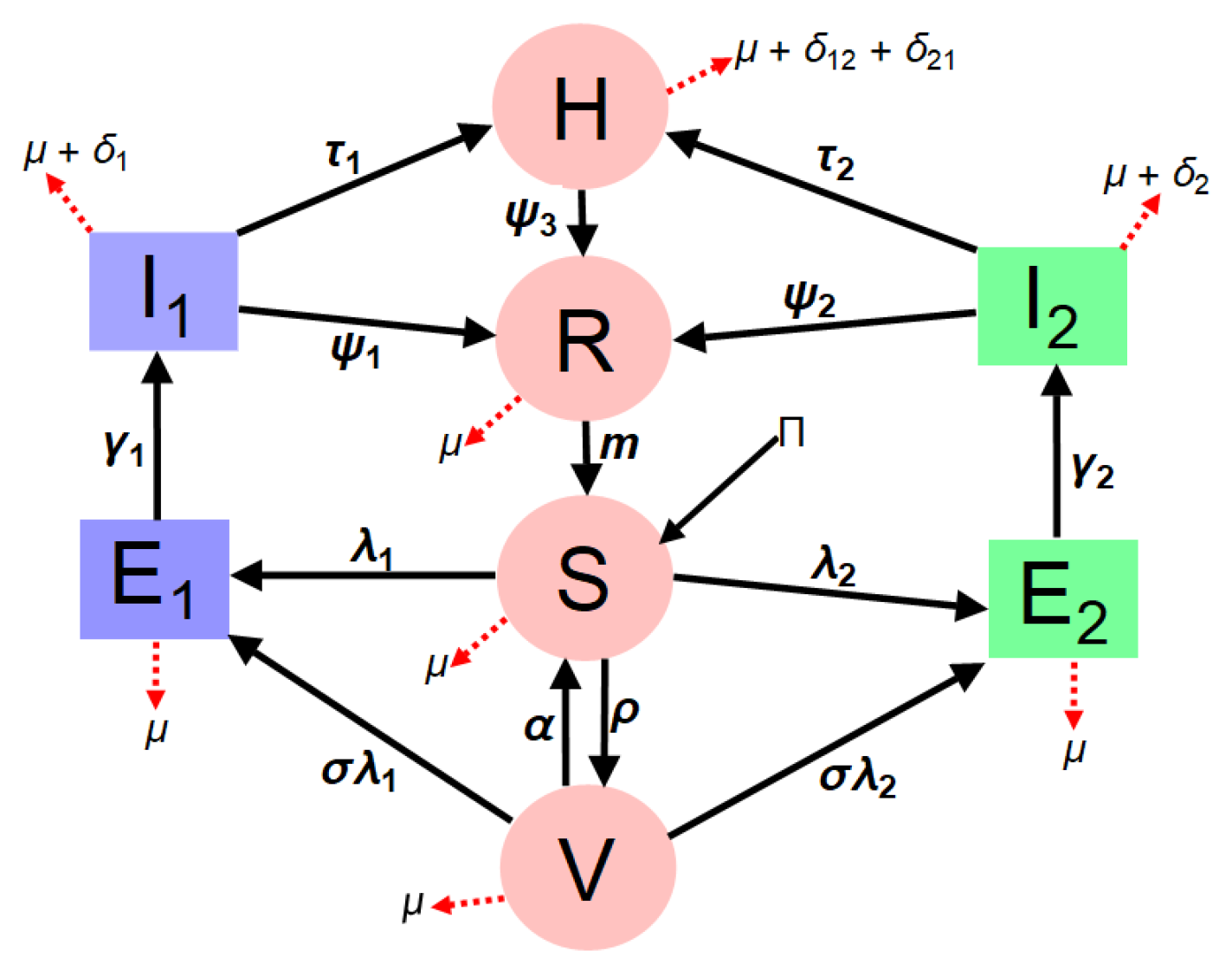
The extended model (3) incorporates the dynamics of dual COVID-19 strains to assess disease impact and mitigation strategies within the entire human population. The total population, denoted as N(t) is divided into distinct compartments: susceptible individuals S(t) who are at risk of infection, vaccinated individuals V(t) who have completed their vaccination, hospitalized individuals H(t) representing active cases requiring medical care, and recovered individuals R(t). Additionally, due to the presence of dual variants, the model stratifies the exposed and infectious compartments into two strains: naive (Eta) strain 1, characterized by exposed/latent individuals () and infectious individuals (), and emerging (Delta) strain 2, represented by exposed/latent individuals () and infectious individuals (). This structured approach allows for a comprehensive analysis of how different strains interact and spread within the population. Therefore,
In model (3), the parameter represent the rate at which individuals are recruited to the population, assuming all newcomers are susceptible. Individuals in all stages of the disease undergo natural death or removal at a rate of . Meanwhile, individuals in the population contract the infection at a rate of or (defined as the force of infection), expressed as follows:
For (Eta) strain 1, represents the effective contact rate linked to disease transmission by symptomatically infectious individuals, and is a modifier accounting for the variability in disease transmission by hospitalized infectious individuals compared to symptomatic individuals. Similarly, for (Delta) strain 2, represents the effective contact rate related to disease transmission by symptomatically infectious individuals for strain 2, while is a modifier considering the variability in disease transmission by hospitalized infectious individuals for the Delta variant (strain 2).
Susceptible individuals in the population are vaccinated at a rate of and move to the vaccinated compartment. Individuals in this compartment can still be infected with either strain 1 or strain 2 of SARS-CoV-2 at a rate of . The population of vaccinated individuals is further reduced due to immunity waning back to the susceptible population at . However, denotes the rate at which newly-infected individuals progress to the infectious compartment for both strain 1 and strain 2. Infectious individuals recover at a rate of and die from the disease at a rate of for both the naive (Eta) strain and the emerging (Delta) strain 2. The hospitalized compartment expands as infectious individuals progress at a rate of , and individuals in this compartment suffer disease-induced mortality at a rate of for both the Eta and Delta variants, as infectious individuals are admitted regardless of the strain of the disease. Furthermore, the recovered compartment expands as individuals who self-medicate move from the infected compartment for both strain 1 and strain 2 to the recovery compartment at a rate of for both existing variants without hospitalization.
Based on the epidemiology of SARS-CoV-2 disease, recovered individuals do not retain permanent immunity against SARS-CoV-2 disease. Hence, individuals with waning immunity revert to the susceptible compartment at a rate of m. Thus, the model is expressed as follows:
Figure 1 illustrates the model formulation for dual-strain SARS-CoV-2 dynamics.:
3. Parameter Estimation and Model Fitting
The developed dual-strain epidemiological model (3), constructed to capture the transmission dynamics of SARS-CoV-2 in Nigeria, is calibrated and validated using empirical data obtained from credible sources such as the Nigeria Centre for Disease Control (NCDC) and the World Health Organization (WHO) [33]. In addition, cumulative COVID-19 data from 2020 to 2021 provide valuable insights into the transmission trajectory and key epidemiological indicators, including infection and recovery rates. These data facilitate robust model fitting and enable reliable forecasting of disease trends, evaluation of intervention effectiveness, and anticipation of potential future outbreaks.
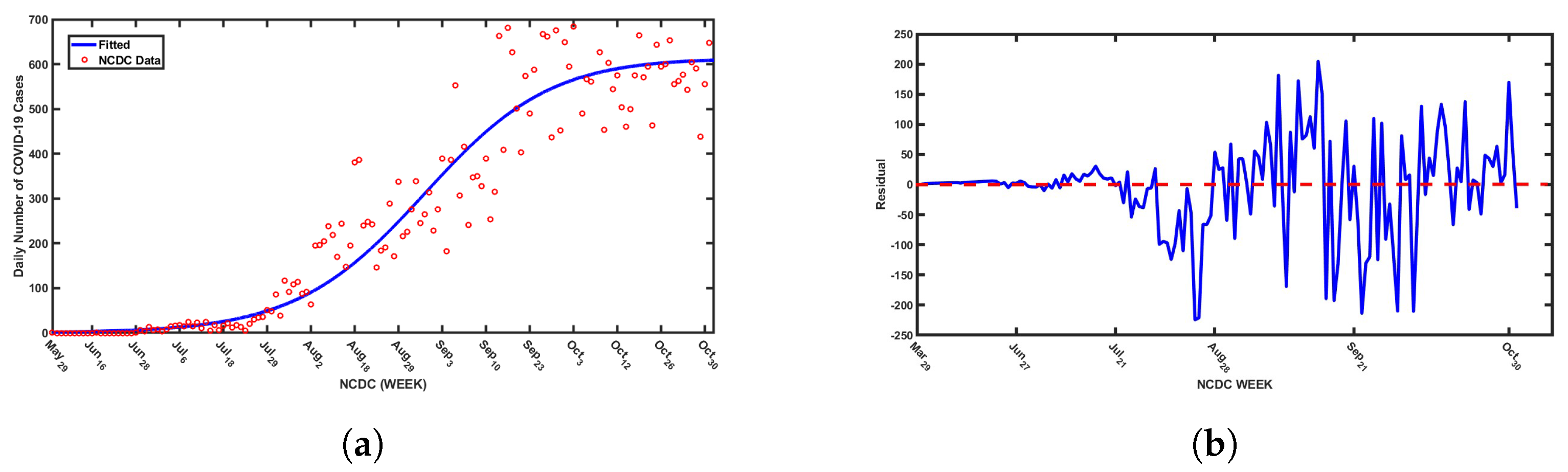
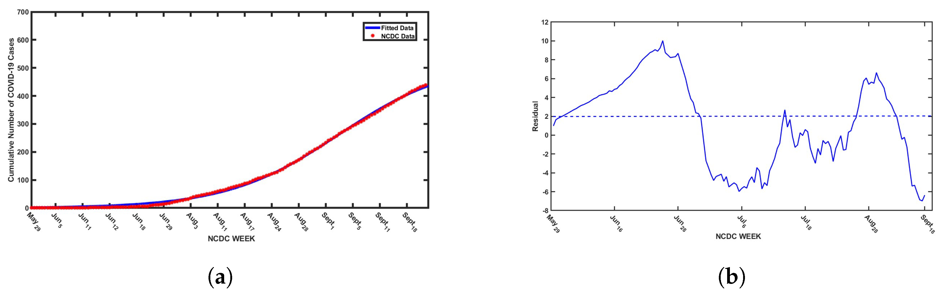
This validation process leverages a nonlinear least squares optimization method to fine-tune the model parameters, ensuring accuracy in reflecting actual infection trends. In particular, confirmed COVID-19 cases in Nigeria, which represent infectious individuals, are used as inputs for calibrating the model. The fitting procedure employs MATLAB’s “lsqcurvefit” function—a powerful tool specifically designed to minimize the sum of squared deviations between observed data points and the corresponding model-generated values. This function refines parameter estimates by iteratively adjusting them to reduce the discrepancy between real and predicted data points, optimizing the fit for both daily and cumulative case counts reported by the NCDC. The results obtained for unknown and known parameter values are presented in Table 1, with model fits illustrated in Figure 2 and Figure 3. However, it is worth noting parameter selection is guided by the importance of parameters in capturing SARS-CoV-19 transmission dynamics, especially in a population with more than one strain of SARS-CoV-2. However, there are 20 biological parameters associated with the proposed model; some of the parameters () were obtained from available literature, while unknown parameters, such as , and , are presented in Table 1. Based upon available information, the initial conditions for the variables of the model are set at , and . Moreover, the fitted curve is depicted in Figure 2 and Figure 3.

Table 1.
Baseline values of the parameters used in Model (3).
Figure 2.
(a)Daily SARS-CoV-2 cases in Nigeria from May 2020 to October 2021 with the best fitted curve from simulations of the proposed model and (b) the residuals for the best fitted curve.
Figure 3.
(a) Cumulative daily SARS-CoV-2 cases in Nigeria from May 2020 to September 2021 with the best fitted curve from simulations of the proposed model and (b) the residuals for the best fitted curve.
Furthermore, we adopted the residual function from MATLAB to obtain the residual plots presented in Figure 2b and Figure 3b to assess the goodness of fit of the model by visualizing the differences (residuals) between observed data points and model-predicted values. The plots illustrate a consistent pattern in the residuals, which appear to be randomly dispersed above and below the horizontal axis. This type of distribution indicates a good model fit. Residuals play a crucial role in identifying unusual observations and evaluating whether the assumptions underlying linear regression, particularly those related to the error term, are satisfied. Observations with high leverage tend to influence the regression line, often resulting in smaller residuals due to their effect on the model’s alignment with the data. In this context, the residuals reflect the vertical differences between the observed data points and the values predicted by the model. Therefore, residuals randomly distributed on both sides of the baseline support the validity of the model fit, as demonstrated in Figure 2 and Figure 3.
3.1. Optimal Control Model (OCM)
In an effort to mitigate the spread of dual-strain COVID-19, the extended Optimal Control Model (OCM) incorporates three key control measures vaccination, implementation of non-pharmaceutical interventions (NPIs), and effective treatment—into the baseline epidemiological model (Equation (3)). This extension aims to assess the impact of these control strategies on disease dynamics, providing a framework for optimizing intervention efforts while considering feasibility and cost-effectiveness. By integrating these controls, the model offers a comprehensive approach to understanding how targeted public health measures can reduce transmission and reduce the burden of disease in the population. The vaccination control strategy, denoted by , is incorporated into the susceptible compartment to maximize the number of individuals who receive vaccination. This strategy aims to accelerate immunity acquisition, thereby reducing the pool of individuals vulnerable to infection. By increasing vaccine uptake, the model evaluates how immunization efforts contribute to the reduction in the overall prevalence of the disease, in addition to limiting the spread of both strains of the virus.
The second control strategy, represented by , accounts for the implementation of NPIs such as social distancing, mask mandates, and lockdown measures. This control is integrated into the force of infection to curtail the number of new infections in the population. NPIs serve as crucial tools, especially in scenarios where vaccine coverage is insufficient or when emerging variants compromise vaccine efficacy. The model assesses how varying levels of NPIs influence transmission rates and contribute to disease suppression. The third control strategy, denoted by , represents the effectiveness of medical treatment and is incorporated into the hospitalized compartment. This measure ensures that individuals receiving treatment have a higher probability of recovery, thereby reducing mortality and minimizing prolonged disease transmission. Effective treatment strategies include antiviral therapies, improved hospital care, and timely medical interventions. By optimizing this control, the model evaluates how access to treatment and healthcare resources can mitigate severe outcomes and contribute to overall disease control. By integrating these three control strategies, the OCMprovides a robust framework for understanding the interplay between vaccination, NPIs, and treatment efforts in managing the dual-strain COVID-19 pandemic. Therefore, the governing system of the ordinary differential equation is expressed as follows:
The initial conditions given for the corresponding state variable at time are , and , while the model parameters are defined in Table 2.
Table 2.
Description for the each control variable.
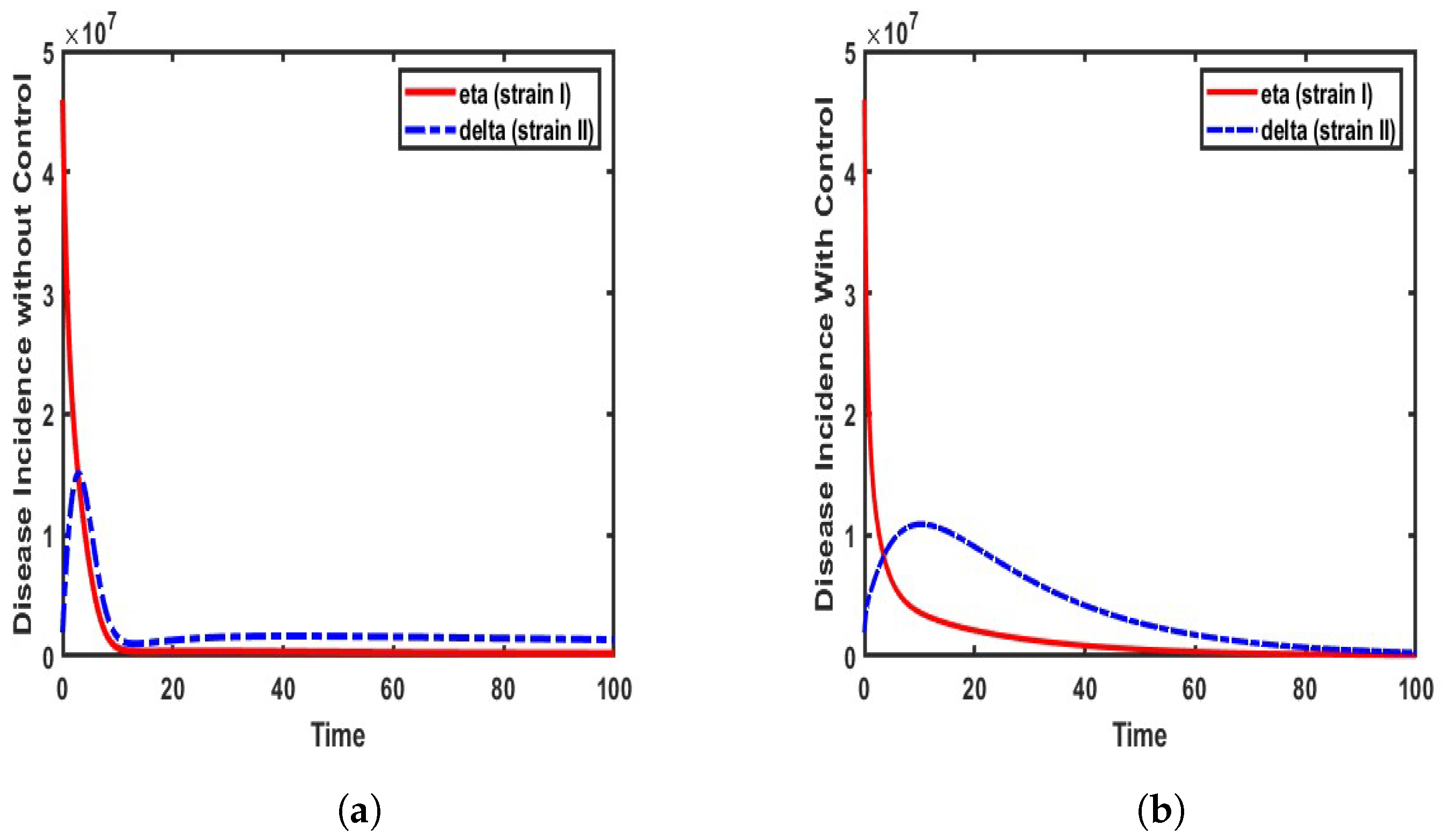
The incidence rates of COVID-19 strains (Eta and Delta) are analyzed based on the formulated model (4). This analysis is conducted under two distinct scenarios:
The results, as illustrated in Figure 4, highlight the variations in transmission dynamics under these conditions. Our findings align with the observations reported by the World Health Organization [6], which emphasize the high transmissibility of the Delta variant. Thus, when the Delta strain first emerged in Nigeria, its rapid spread outpaced that of previous Eta variants, making it a dominant strain within a short period. This reveals the heightened infectiousness of the Delta variant compared to the Eta strain, particularly in populations like Nigeria, where mitigation strategies were not promptly enforced.
As illustrated in Figure 4a, the incidence rate of Eta (strain I) gradually declines following the emergence of the Delta strain in the population. The Delta strain exhibits steady growth, reaching a rate of approximately 1.5 million infected individuals before subsequently declining. This trend is observed when the model is simulated without control measures, using the parameter values specified in Table 1. In contrast, Figure 4b shows a more rapid decline in the incidence rate of the Eta strain, while the rise of Delta strain II is effectively mitigated, limiting infections to approximately 1 million individuals. This reduction is attributed to the implementation of control measures.
3.2. Optimal Control Problem Formulation
Here, the objective functional is formulated with control terms expressed in a quadratic form, aligning with conventional approaches commonly adopted in existing research [34,35,36]; thus, the model’s objective functional is defined as follows:
and
such that
, and are Lesbeque measurable functions; and , and for is the control set. Defining t as the final time, , and are the weight constants of susceptible individuals, individuals infected with strain I, individuals infected with strain II, and hospitalized individuals respectively. The weights indicate the relative importance of reducing specific population classes to effectively control the spread of COVID-19 within Nigeria, while , are the weights designed to reflect the relative costs or efforts associated with implementing each time-dependent control strategy. For the purposes of this study, we assume hypothetical values for these upper limits: , . These values are chosen based on the assumption that they are realistically achievable given the available resources.
However, the primary objective of this study is to find the optimal combination of effectiveness levels for control measures and , and this involves balancing the minimization of implementation costs with the maximization of vaccination coverage using a highly effective vaccine. Furthermore, it aims to promote hospitalization for those infected with either strain of the disease through enhanced public awareness campaigns and ensure that infected individuals receive appropriate treatment. The mathematical induction and proof for model (3) and the optimal control model (5) are presented in Appendix A.
4. Numerical Simulation
The model simulations are conducted using parameter values from existing literature, while parameters not available in the literature are inferred based on logical proportionality assumptions. The optimality system is defined by integrating the model system (Equation (5)), the adjoint equations, and the control characterizations (Equation (A19)), implemented in MATLAB R2022B using the forward–backward sweep method introduced by Lenhart and Workman [34]. This process involves a 10-dimensional system of ordinary differential equations, governed by both initial and transversality conditions. The iterative scheme, progressing from forward to backward, follows the methodology outlined in [36,37], using the fourth-order Runge–Kutta numerical method. The parameters used in this analysis are presented in Table 2. Our study investigates the prevalence of the disease within the population by incorporating control variables into the dynamics of human interactions. The initial conditions for the state variables are set as follows: S = 218,186,856, , = 200,000, , = 150,000, , , and , with a final time horizon of 300 days.
The weight coefficients and cost functional are assigned as , , , , = 12,000, = 90,000, and = 10,000. Thus, we assume that , indicating that the cost of vaccines and the implementation of a vaccination program is higher than the cost of non-pharmaceutical interventions (NPIs) and the effective treatment of infected individuals, respectively.
The formulated model (3) evaluates individual control strategies, as well as combinations of interventions, to mitigate the prevalence of COVID-19 while considering their associated costs.
4.1. Single Control Strategy
In this section, we examine the influence of a single control strategy on the dynamics of COVID-19 within the population. Our analysis specifically focuses on assessing the overall burden that both strains of COVID-19 impose on the population by evaluating disease prevalence. To achieve this, we consider the impact of implementing a single control measure at a time, namely vaccination, adherence to non-pharmaceutical interventions (NPIs), or treatment. By isolating the effect of each strategy, we aim to gain insights into its effectiveness in mitigating disease spread and reducing case numbers. The implementation of this approach is illustrated in Figure 5, Figure 6 and Figure 7.
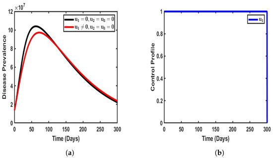
Figure 5.
Impact of single control when . (a) Vaccination-only approach; (b) vaccination-only profile.

Figure 6.
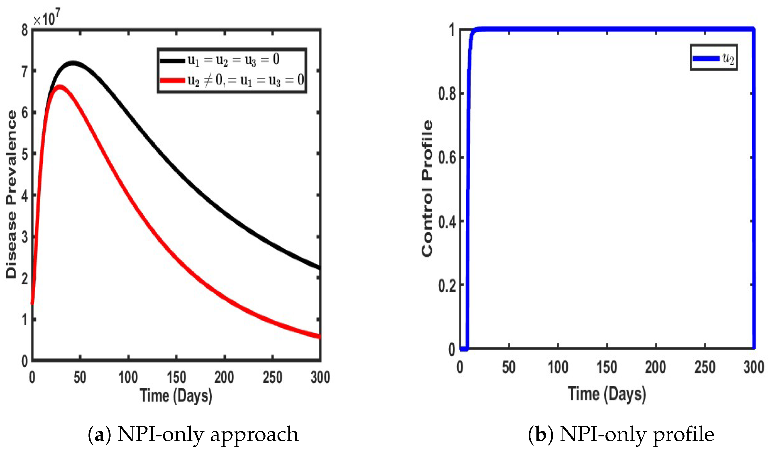
Impact of single control when .

Figure 7.
Impact of single control when .
By introducing vaccination as the only strategy to mitigate the burden of COVID-19 in the population (), a significant reduction in disease prevalence was observed compared to scenarios where no control measures were applied. The implementation of vaccination led to a notable decline in the number of infected individuals, effectively reducing the prevalence of dual-strain COVID-19 within the population. Specifically, the total number of infected individuals decreased from an estimated 10.1 million to approximately 8.9 million, thereby preventing around 1.5 million people from contracting either strain of the virus.
The impact of vaccination as a control measure is further highlighted in Figure 5b, which illustrates the control profile over time. The strategy initially maintains a high level of effectiveness, stabilizing at its peak for an extended period of approximately 300 days before gradually declining. This suggests that while vaccination plays a crucial role in curbing disease transmission and reducing infection rates, its long-term efficacy may diminish over time due to factors such as waning immunity, potential variations in vaccine uptake, or the emergence of new variants. Moreover, the observed stabilization period indicates that a sustained and consistent vaccination effort is required to achieve long-term disease suppression. Without periodic reinforcement through booster doses or complementary interventions, the effectiveness of vaccination alone may not be sufficient to fully eradicate the disease. Thus, while vaccination serves as a powerful tool in mitigating the spread of COVID-19, its success is contingent upon factors such as continued public compliance, the availability of booster programs, and the potential need for adaptive strategies to address evolving epidemiological challenges.
As illustrated in Figure 6, when non-pharmaceutical interventions (NPIs), denoted as , are implemented as the only control strategy, a noticeable delay occurs in the time taken for the disease to reach its peak prevalence. This delay is in stark contrast to scenarios where no intervention is applied, indicating that NPIs play a crucial role in slowing the transmission of the virus within the population. The enforcement of NPIs—such as social distancing, mask mandates, movement restrictions, and hygiene protocols—reduces the immediate exposure rate, thereby extending the time it takes for the infection to reach a significant proportion of individuals.
However, while NPIs effectively slow the rate of infection, their impact in terms of reducing the total number of infected individuals appears to be relatively modest compared to other control strategies. The preventive effect of NPIs alone results in only a slight reduction in the number of individuals infected with both strains of COVID-19. This suggests that while NPIs help mitigate the rapid spread of the virus, they may not be as effective as vaccination or treatment in significantly reducing the prevalence of overall disease. One potential reason for this limitation is that NPIs rely largely on behavioral compliance, which can be inconsistent across different demographics and over long periods. Furthermore, NPIs do not directly confer immunity, making them more effective when used in conjunction with other control measures rather than as a standalone approach.
Figure 6b provides further insight into the control dynamics of NPIs over time. Initially, there is a slight stabilization in the effectiveness of NPIs, maintaining a relatively steady impact for the first 25 days of implementation. However, after this initial period, the effectiveness of NPIs declines sharply to its lowest point over a prolonged period. This decline suggests that long-term adherence to NPIs is challenging, as factors such as economic constraints, public fatigue, and policy relaxations contribute to reduced compliance over time. Interestingly, around day 250, the control effect of NPIs resurges to a peak before eventually subsiding again. This fluctuation could be attributed to temporary reinforcements of public health measures in response to increased infection rates, followed by subsequent relaxations as cases decline.
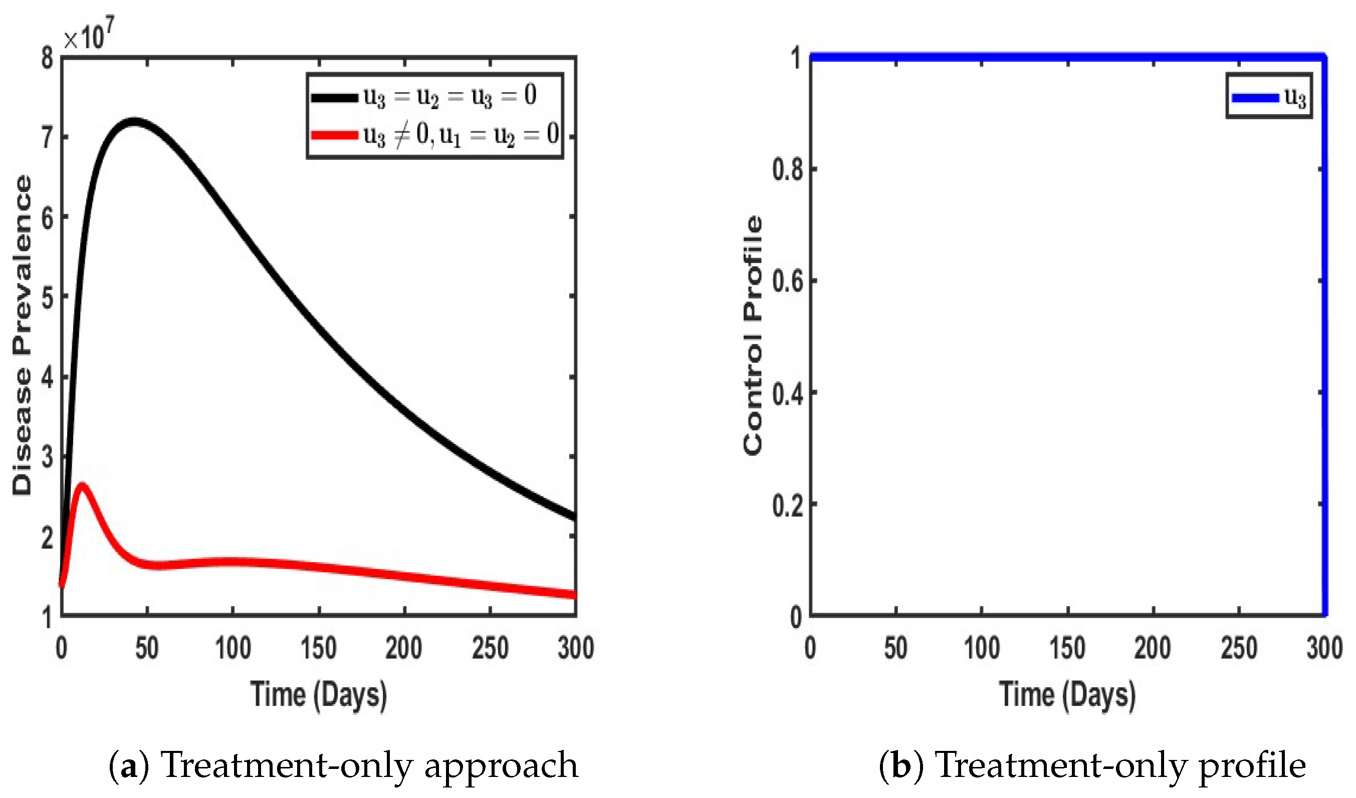
Figure 7 illustrates the impact of treatment as the sole intervention in curbing the spread of the dual-strain disease within the population. As depicted in Figure 7a, the implementation of treatment as the only control strategy significantly reduces the overall burden of the disease compared to scenarios where no intervention is applied. Treatment plays a critical role in not only reducing the severity of infections but also in limiting further transmission by shortening the infectious period of affected individuals. This, in turn, decreases the number of actively transmitting cases within the population.
In the absence of any control measures, the prevalence of the disease exhibits an exponential rise, reaching approximately 10.5 million infected individuals before gradually declining. This pattern suggests that, without intervention, the disease follows a natural course of rapid spread until factors such as population immunity or resource depletion begin to slow transmission. However, when treatment is introduced as the sole control measure, a stark contrast is observed—the prevalence of the disease does not experience the same uncontrolled surge. Instead, treatment actively mitigates disease spread, leading to a substantial reduction in the number of infected individuals over time. This highlights the effectiveness of treatment in minimizing the overall disease burden and reducing the strain on healthcare systems.
Moreover, the treatment control profile, as illustrated in Figure 7b, reveals a sustained level of efficiency throughout the period of implementation. The control remains steady for approximately 300 days, indicating that treatment continues to be effective in reducing infections and improving recovery rates for an extended duration. This stability suggests that as long as treatment remains widely accessible and adequately administered, its impact on disease suppression can be maintained. However, after this period, a gradual decline in control efficacy is observed, reducing to its lowest level. This could be attributed to factors such as treatment saturation, potential resistance to therapeutic interventions, or limitations in healthcare capacity over prolonged periods.
4.2. Dual Control Strategy
In this section, we analyze the impact of combining two control strategies—either vaccination and treatment, vaccination and NPIs, or treatment and NPIs—to effectively assess their influence in terms of reducing the prevalence of the disease burden. By implementing these dual control strategies, we aim to determine how their synergistic effects contribute in terms of mitigating the spread of the dual-strain disease compared to when each strategy is applied in isolation. This approach allows us to evaluate the extent to which these interventions complement each other, potentially enhancing disease suppression and improving overall public health outcomes.
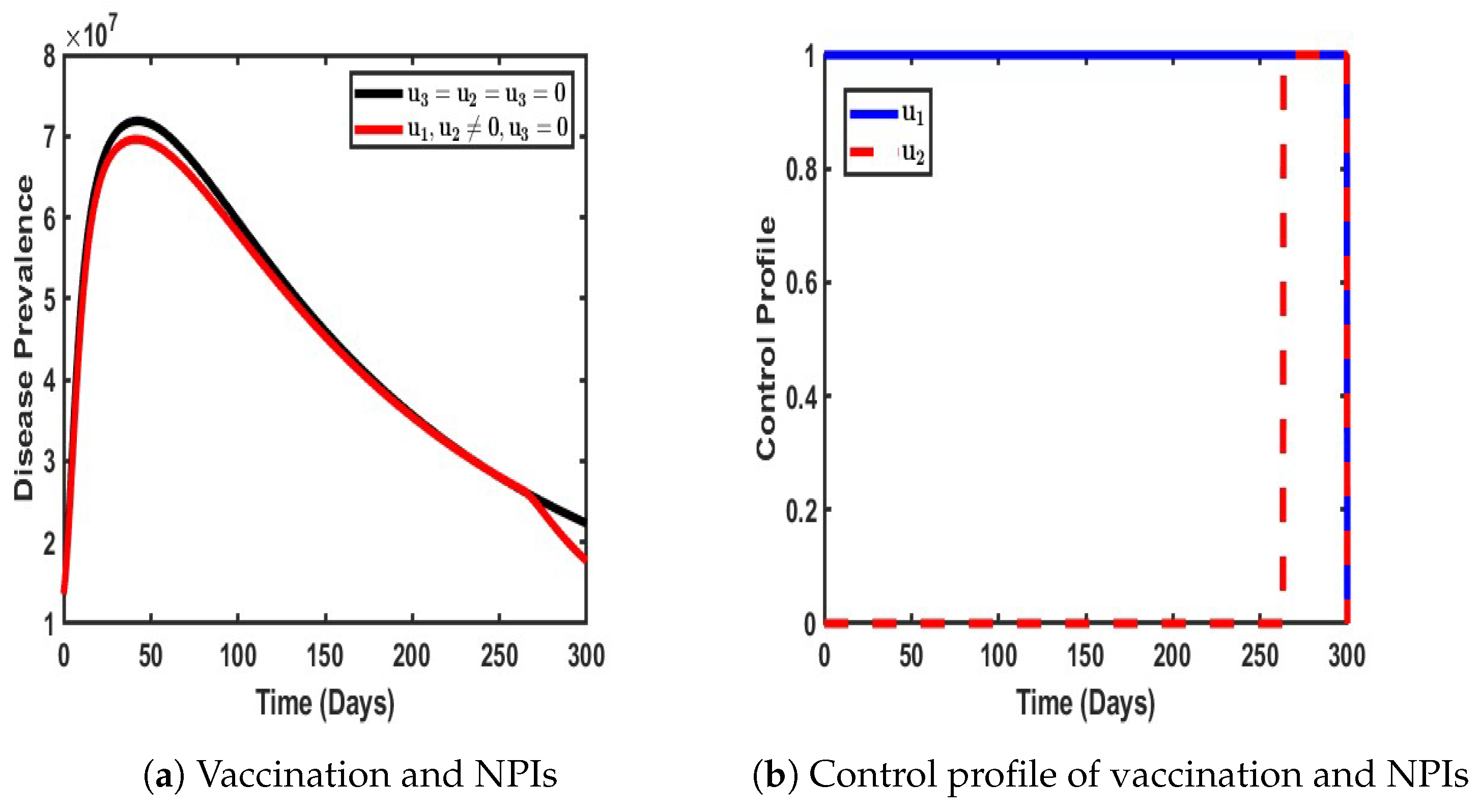
As illustrated in Figure 8, the combined implementation of vaccination and non-pharmaceutical interventions (NPIs) was strategically employed to mitigate the prevalence of the COVID-19 dual-strain disease burden. The impact of these control measures was evident, as the population of infected individuals (represented by the red solid line) declined significantly. Specifically, in the absence of any intervention, the number of infected individuals peaked at approximately 10.2 million. However, when both vaccination and NPIs were enforced in the population, this number reduced to 9.2 million, indicating a measurable decline in disease transmission (see Figure 8a). Furthermore, the control profile, as depicted in Figure 8b, highlights the stability and efficacy of the vaccination strategy at its peak. The profile also reveals the behavior of NPIs, which remained at their lowest possible intensity for an initial period of 299 days before gradually increasing to their peak levels. Notably, after reaching this peak, the efficiency of NPIs exhibited periodic fluctuations over time. This dynamic response indicates the adaptability of NPIs in relation to real-time epidemiological conditions, reinforcing the necessity of a balanced approach combining pharmaceutical and non-pharmaceutical interventions to ensure sustained disease suppression.
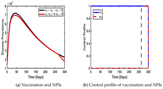
Figure 8.
Impact of dual control with and when .
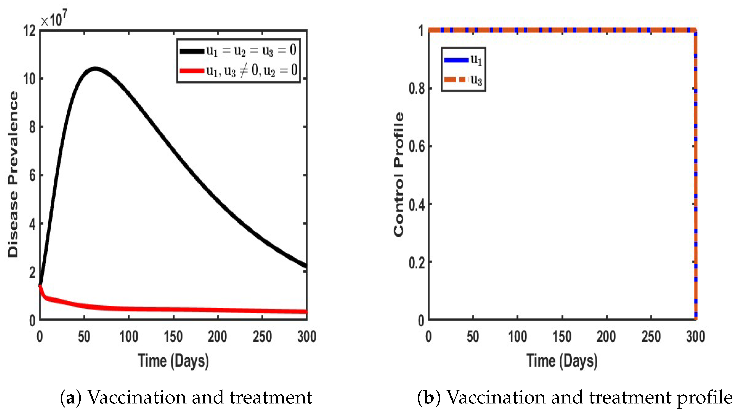
As shown in Figure 9, in a similar pattern, the combined strategy of vaccination and treatment was implemented within the dynamic population, and its impact in terms of reducing COVID-19 prevalence was significant. The results indicate a dramatic decline in the number of infected individuals, from an initial peak of 10.1 million to a remarkably low 0.2 million, demonstrating the effectiveness of the adopted control measures (as represented by the red line in Figure 8a).
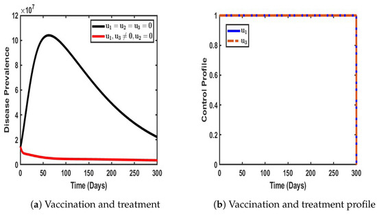
Figure 9.
Impact of a dual control strategy with and when .
Furthermore, Figure 9b reveals the stability and sustained efficacy of the control strategy during the initial 30-day period. Beyond this phase, both vaccination and treatment efforts gradually declined to their minimum levels, suggesting a shift in intervention intensity over time. This pattern underscores the potential of a well-calibrated vaccination and treatment strategy to achieve substantial disease suppression while also highlighting the need for continuous assessment to maintain long-term epidemiological control.
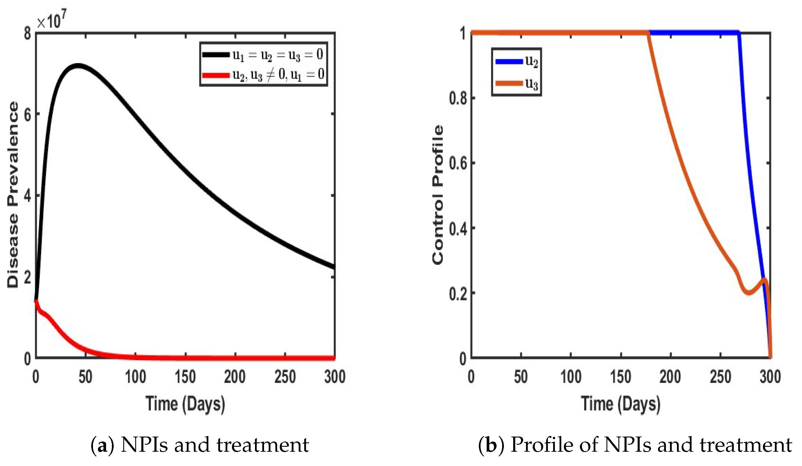
As shown in Figure 10, our objective was to evaluate the effectiveness of a dual control strategy that incorporates both non-pharmaceutical interventions (NPIs) and effective treatment for individuals infected with either strain of COVID-19. This combined approach was designed to mitigate the overall disease prevalence within the population by targeting both infection prevention and recovery enhancement.

Figure 10.
Impact of a dual control strategy with and when .
A closer examination of Figure 10a reveals that the implementation of these control measures had a profound impact in terms of reducing the disease burden. Specifically, the number of infected individuals declined significantly compared to scenarios where no control measures were in place. In the absence of intervention, the number of infections experienced a sharp and continuous rise, exacerbating disease transmission and increasing the overall burden on healthcare systems. However, with the application of NPIs and treatment, a substantial reduction in the number of infected individuals was observed, demonstrating the effectiveness of this dual strategy in curbing disease spread (see Figure 10a).
Furthermore, the control profile illustrated in Figure 10b provides deeper insights into the stability and duration of these interventions. Notably, both control measures remained at their peak levels for approximately 150 days, indicating a sustained period of optimal intervention where transmission suppression and patient recovery were maximized. Beyond this period, treatment efforts began to decline, suggesting either a strategic relaxation of treatment measures or a shift in disease dynamics that required lower intervention intensity. Subsequently, NPIs maintained their effectiveness for a longer duration but eventually began to decline after approximately 280 days.
4.3. Triple Control Strategy
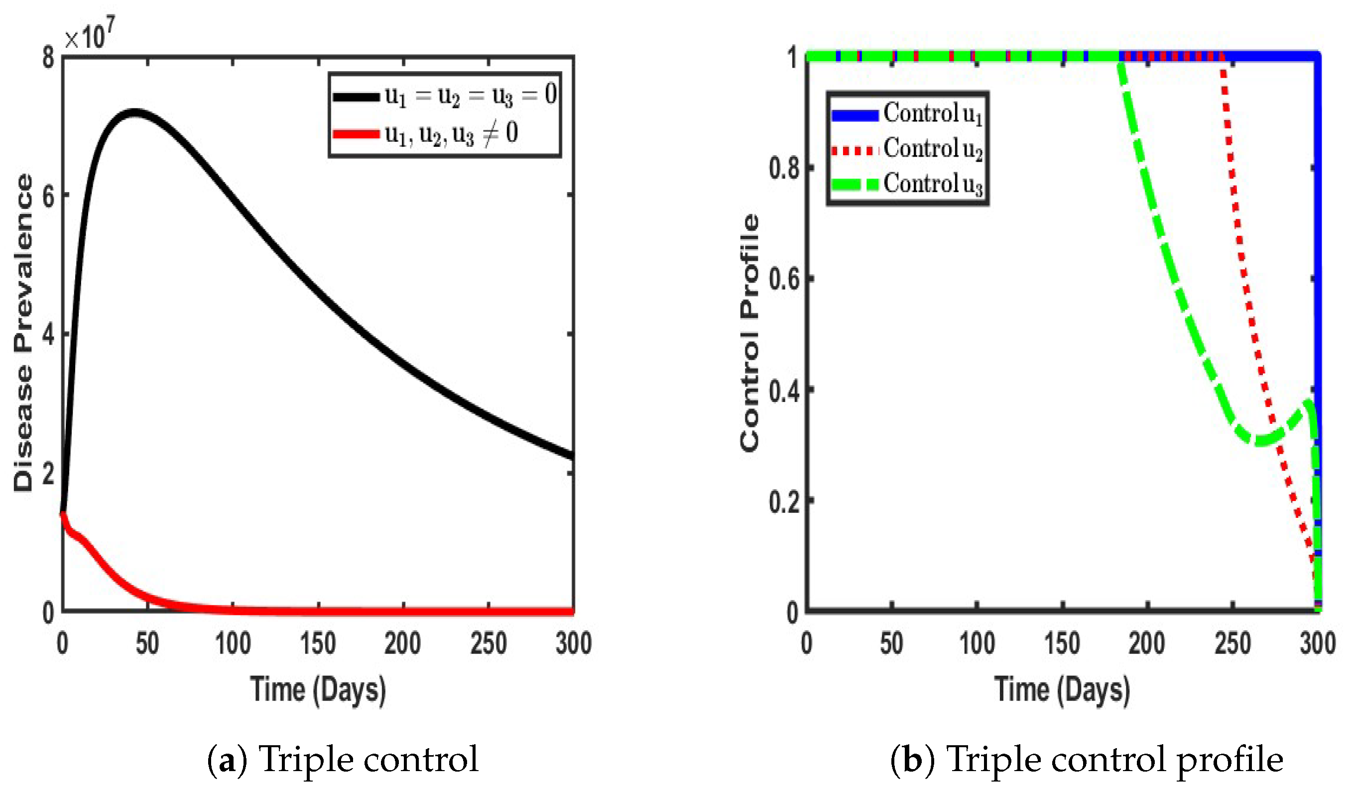
This approach integrates all three strategies—non-pharmaceutical interventions (NPIs), vaccination, and effective treatment—into a single control strategy to comprehensively evaluate their collective impact in terms of mitigating the spread of COVID-19 within the population. By combining preventive, therapeutic, and immunization measures, this strategy aims to achieve optimal disease mitigation, ensuring a multi-faceted defense against both strains of the virus.
As illustrated in Figure 11, the simultaneous application of these three control measures yielded a significant reduction in COVID-19 prevalence within the population. The impact was profound, as the number of infected individuals was drastically reduced to its lowest recorded levels, approaching what could be considered the near elimination of active infections. This finding underscores the critical synergy between vaccination, NPIs, and treatment; vaccination curtails susceptibility, NPIs limit transmission, and treatment enhances recovery, working collectively to drive the infection rate to its minimal threshold. Furthermore, the control profile, as depicted in Figure 11b, provides insights into the temporal stability and efficiency of each intervention. Each control measure initially maintained a stable peak, indicating their sustained effectiveness in containing disease spread during the early phase of implementation. However, as the prevalence of the disease decreased, the necessity for each intervention diminished, leading to a gradual reduction in the intensity of the control. Interestingly, these declines did not occur simultaneously; instead, each strategy began to taper off at different intervals, suggesting a dynamic adaptation of control efforts based on evolving epidemiological conditions.
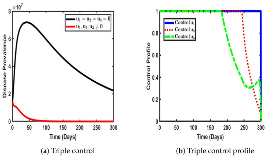
Figure 11.
Impact ofa triple control strategy ().
5. Cost-Effectiveness Analysis
Cost-Effectiveness Analysis (CEA) is a tool for comparing the costs and outcomes of different interventions to determine the most efficient strategy. Commonly applied in healthcare, public policy, and business, CEA helps identify strategies that maximize benefits while minimizing costs. However in this section, CEA is used to evaluate the effectiveness of non-pharmaceutical interventions (NPIs), vaccination, and treatment programs in mitigating the spread of COVID-19, allowing for direct comparison of interventions with the same goal. For cost-effective analysis, we calculate the efficiency index (EI) and incremental cost-effectiveness ratio (ICER).
5.1. Efficiency Analysis of the Strategies
In this section, efficiency analysis is applied to identify the most effective control measure that prevents the greatest number of infections, irrespective of implementation costs. The control measure with the highest efficiency is regarded as the optimal choice among all available options. In simple terms, the intervention with the highest Efficiency Index (E.I) is considered the best control. For this analysis, the Efficiency Index (E.I) is defined as follows:
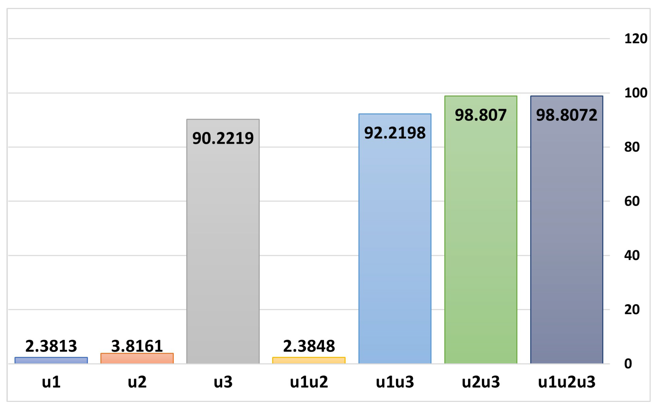
Table 3 provides a detailed evaluation of the effectiveness of various control strategies—both single strategies and combined strategies for the management of dual-strain COVID-19 infections. Among single control strategies, implementing non-pharmaceutical interventions (NPIs), denote by , averted approximately 1.497 billion cases of infection, and the vaccination control strategy () alone prevented 2.399 billion cases, while treatment control strategy () appears to be the most efficient single strategy, averting a remarkable 56.73 billion cases of infection. For combinations of two control strategies, NPIs combined with vaccination averted 1.5 billion cases; NPIs and treatment prevented 57.986 billion cases; and vaccination paired with treatment proved to be the most efficient dual-strategy approach, averting 62.128 billion cases of infection. However, When all three controls (NPIs, vaccination, and treatment) were combined, they collectively averted 62.128 billion cases, achieving an Efficiency Index (EI) of 98.8072. This makes the combination of all three controls the most effective and comprehensive strategy for curbing COVID-19 infections, followed closely by the dual vaccination and treatment strategy. Overall, these findings highlight the significant role of treatment in both single and combined strategies and the unparalleled efficiency of a holistic, multi-control approach in managing the pandemic, as presented in Figure 12.
Table 3.
Efficiency Index table for applied control measures.
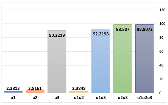
Figure 12.
Efficiency Indices for selected controls obtained through Equation (7).
5.2. Incremental Cost-Effectiveness Ratio (ICER)
The incremental cost-effectiveness ratio (ICER) measures the ratio between costs and health benefits of any two interventions competing for the same limited resources. The calculation of the ICER makes use of the following formula:
In the context of evaluating two competing strategies, say J and G, and supposing that strategy G demonstrates greater effectiveness compared to strategy J (mathematically expressed as ), the incremental cost-effectiveness ratio (ICER) serves as a critical metric for comparing the two strategies. The ICER quantifies the additional cost required to achieve an additional unit of effectiveness when moving from the less effective strategy (J) to the more effective one (G). The ICER for strategy J is often referred to as the baseline strategy, which is calculated by dividing its total cost () by its total effectiveness ():
For strategy G, which is more effective, the ICER is calculated incrementally by comparing it directly to strategy J. This involves subtracting the total cost of strategy J from that of strategy G and dividing the result by the difference in their effectiveness:
This method has been applied to determine the most cost-effective intervention in the control of diseases by a number of researchers [24,27,29,31]. Using the simulation results with budget cost for NPIs, vaccination, and treatment , we ranked our control strategies in order of the number of averted infections (in increasing order), as presented in Table 4.
Table 4.
Summary of applied control strategies for first iteration.
Control strategy is compared with control strategy with respect to increased effectiveness and in reference to Table 4.
Control strategy is less effective compared to control strategy , as indicated by the fact that . Consequently, control strategy is excluded from the set of viable control options under consideration, as presented in Table 5.
Table 5.
Summary of applied control strategies for second iteration eliminating .
Next, we compare control strategy with control strategy . The ICER values for strategy and control strategy are calculated below using values from Table 5:
Thus, control strategy is less effective than control strategy , since . Hence, control strategy is eliminated from the set of control options to be considered.
Furthermore, we compare control strategy with control strategy . The ICER values for strategy and control strategy are calculated below using values from Table 6:
Thus, control strategy is less effective than control strategy , since . Hence, control strategy is eliminated from the set of control options to be considered.
Table 6.
Summary of applied control strategies for third iteration eliminating .
The analysis of the control strategies presented in Table 7 for the management of a dual-strain COVID-19 outbreak provides insights with respect to cost-effectiveness and infection reduction. The results suggests that different combinations of intervention yield varying levels of efficiency in terms of total infections averted, total costs incurred, and the incremental cost-effectiveness ratio (ICER). The intervention strategy labeled alone is the least costly but also the least effective, preventing only billion infections. When is combined with , i.e., , the total number of infections averted increases to billion at a slightly higher cost of USD10.99 billion. This strategy demonstrates a reasonable balance between cost and effectiveness, with an ICER of , making it a cost-effective option for Nigerian governments or organizations operating under financial constraints. For instances where Nigerian governments/policymakers are aiming for maximum infection reduction, the combination of all three interventions () is the most effective, preventing billion infections. However, this comes at a significant cost of USD50.04 million and an ICER of , indicating diminishing cost-effectiveness as additional interventions are implemented. While this approach is the most resource-intensive, it is justified in scenarios where minimizing infections is the top priority, such as during peak waves of a pandemic.
Table 7.
Summary of applied control strategies for fourth iteration eliminating .
A middle-ground approach is represented by , which prevents billion infections at the same cost of USD46.38 million but with a slightly lower ICER of 0.00075. This strategy is ideal for policymakers who seek high effectiveness without implementing all three interventions, particularly if one intervention () is difficult to enforce or sustain. While not as effective as , it offers nearly the same level of infection prevention at a slightly better cost-effectiveness ratio. From a policy perspective, the best approach depends on the available budget and the public health priorities of a given nation. Governments or organizations with financial limitations should prioritize , as it provides a significant reduction in infections at a manageable cost. In contrast, if the objective of the Nigerian government is to achieve the highest possible reduction in infections, then is the most suitable choice, despite its high cost. For governments seeking a balance between financial feasibility and effectiveness, presents an optimal compromise. Ultimately, these insights offer a data-driven framework for the design and implementation of COVID-19 control policies that align with both economic constraints and public health objectives.
6. Conclusions and Recommendations
In this paper, we have introduced a novel non-linear optimal control model for the dynamics of dual-strain COVID-19, incorporating vaccination, non-pharmaceutical interventions (NPIs), and effective treatment strategies for actively infected individuals. Our analysis confirms that the model is both mathematically and epidemiologically well-posed. Using optimal control theory and Pontryagin’s Maximum Principle, we conducted a rigorous theoretical examination of the non-autonomous system. To assess the influence of time-dependent control measures on disease prevalence, we performed numerical simulations of the optimality system, a two-point boundary value problem consisting of a 10-dimensional system of ordinary differential equations. These simulations were carried out in three phases: first, evaluating the effects of single control strategies; second, analyzing dual control strategies; and third, assessing the impact of triple control strategies with varying weights and implementation costs to mitigate the spread of multiple strains of COVID-19.
Our findings reinforce the critical importance of a comprehensive and balanced approach to controlling highly infectious diseases. While single control strategies provide only partial containment, their combined application creates a synergistic effect that significantly enhances disease suppression. This insight is particularly valuable for public health policymakers, as it underscores the necessity of a multi-pronged strategy for achieving sustained control and eventual eradication of the disease.
Recommendations
The summary Table 8 outlines the recommended strategies based on cost-effectiveness, infection reduction, and budgetary considerations. The optimal approach varies depending on financial constraints, with a strong recommendation for a dual or triple control strategy to achieve the most significant reduction in disease prevalence while maintaining economic feasibility.
Table 8.
Summary of recommended strategies.
Author Contributions
Conceptualization, O.I.I. and T.T.Y.; Methodology, T.T.Y. and O.I.I.; Software, O.I.I.; Validation; O.I.I. and K.O.; Formal analysis, K.O. and O.I.I.; Investigation, O.I.I., K.M.O. and K.O.; Data curation, O.I.I.; Writing original draft preparation O.I.I.; Writing—review and editing, T.T.Y. and O.I.I.; Visualisation, O.I.I. and K.O.; Supervision, T.T.Y. and K.M.O.; Project Administration, O.I.I. and K.O. All authors have read and agreed to the published version of the manuscript.
Funding
This research received no external funding.
Data Availability Statement
All Data Source are reference in the article.
Acknowledgments
Idisi Oke Isaiah is a doctoral student at the Federal University of Technology, Akure (FUTA). This study forms part of the research conducted for his PhD program. The authors would like to express their sincere appreciation to the editors for their efforts in ensuring the thoroughness and quality of the work.
Conflicts of Interest
The authors declare no conflict of interest.
Appendix A
Appendix A.1. Uniqueness of the Solution
Theorem A1.
Let denote the following domain: .
Proof.
Suppose satisfies the Lipschitz condition; therefore,
Whenever points and belong to the and k is used to represent the positive constant, then there exist a constant () and a unique solution () of model (3) in the interval of . It is important to note that condition (A1) is satisfied by to be continuous and bounded in domain .
If has a continuous partial derivative in a bounded, closed, convex domain (, i.e, the convex set of real numbers, where is used to denote a real number), then it satisfies a Lipschitz condition in . Our interest is in the following domain:
Therefore, we look for the bounded solution of the form . □
Appendix A.2. Existence of a Solution
Theorem A2.
Substituting the state variable on the right side of the model (3) as and taking as the first equation in the model (3), we partially differentiate with respect to the state variables and obtain
The same procedures are undertaken for the remaining equations of model (3). Therefore, all partial derivatives are continuous and bounded; hence, based on Theorem A2, it is concluded that there exists a unique solution to the model in Equation (3) in the domain region (). This method was used in [38]
Appendix A.3. Invariant Region
Theorem A3.
Set Ω is positively invariant and attracts all solutions in .
Appendix A.4. Existence of an Optimal Control Strategy for the Problem
In this section, we examine the sufficient conditions for the existence of the solution to the optimal control problem.
Theorem A4.
There exists an optimal control set with a corresponding solution to the model system (4) that minimizes over .
Proof.
The existence of the optimal control is ensured by the compactness of the control and state variable, as well as the convexity of the problem, according to Theorem A4 and its corresponding corollary proposed by Fleming and Rishel [39]. The following non-trivial requirements of Fleming and Rishel’s theorem are stated and verified as follows:
- The set of all solutions to the model Equations (3), along with its associated initial conditions and the corresponding control functions in , is non empty.
- The state system can be expressed as a linear function of the control variables, with coefficients that depend on time and state variables.
where . □
We refer to Theorem 3.1 from the Picard-Lindelöf framework as presented in [40]. According to this result, if the solutions of the state system are bounded and the system itself is continuous and satisfies the Lipschitz condition with respect to the state variables, then a unique solution exists for every admissible control in set . In our case, each state variable (S, V, E_1, I_1, E_2, I_2, H, R) ∈ Ω is both upper- and lower-bounded, implying that the state solutions are confined within a finite range. Additionally, it can be readily shown that the partial derivatives of the right-hand side of the state equations with respect to the state variables are bounded, confirming the Lipschitz continuity of the system. This satisfies the first requirement. Moreover, a direct inspection of the model equations in (3) indicates that control functions and appear linearly, satisfying the second requirement. As for the third condition, we observe that the integrand () in the objective functional is convex due to its quadratic dependence on the control variables. To complete the verification, it remains to be demonstrated that is bounded, thereby satisfying the final requirement.
Equation (A9) shows that the integrand () is bounded below. Thus, a unique solution to the optimality system exists for small time intervals, given the opposite time orientations of the state and adjoint equations. Furthermore, the uniqueness of the solution to the optimality system ensures the uniqueness of the optimal control if it exists.
Characterization of the Optimal Controls
In this section, we characterize the optimal controls for the three adopted control measures and the corresponding states (). The necessary conditions for these optimal controls are derived using Pontryagin’s Maximum Principle as described in [39,41].
Theorem A5
(Necessary condition). Let be an optimal control with the corresponding states (). Then, there exist the adjoint variables () that satisfy:
and the transversality conditions, i.e.,
with the optimal controls defined as follows:
where
Proof.
The Hamiltonian is maximized with respect to the controls at the optimal control (); thus, we differentiate with respect to on to obtain
Hence, solving for yields
The bonds of , and are imposed on the controls (A24) to obtain
The next step involves solving the optimality system, which comprises the state equations defined in system (4), along with their initial conditions, and adjoint Equations (A10)–(A17), subject to the transversality conditions specified in (A24).
Appendix A.5. Numerical Simulation Plots for Each Compartment of the Control Model
This section presents the simulation plots for each control strategy, illustrating their impact on the model compartments.

Figure A1.
Impact of NPIs only control on each compartment of model (4).
Figure A1.
Impact of NPIs only control on each compartment of model (4).
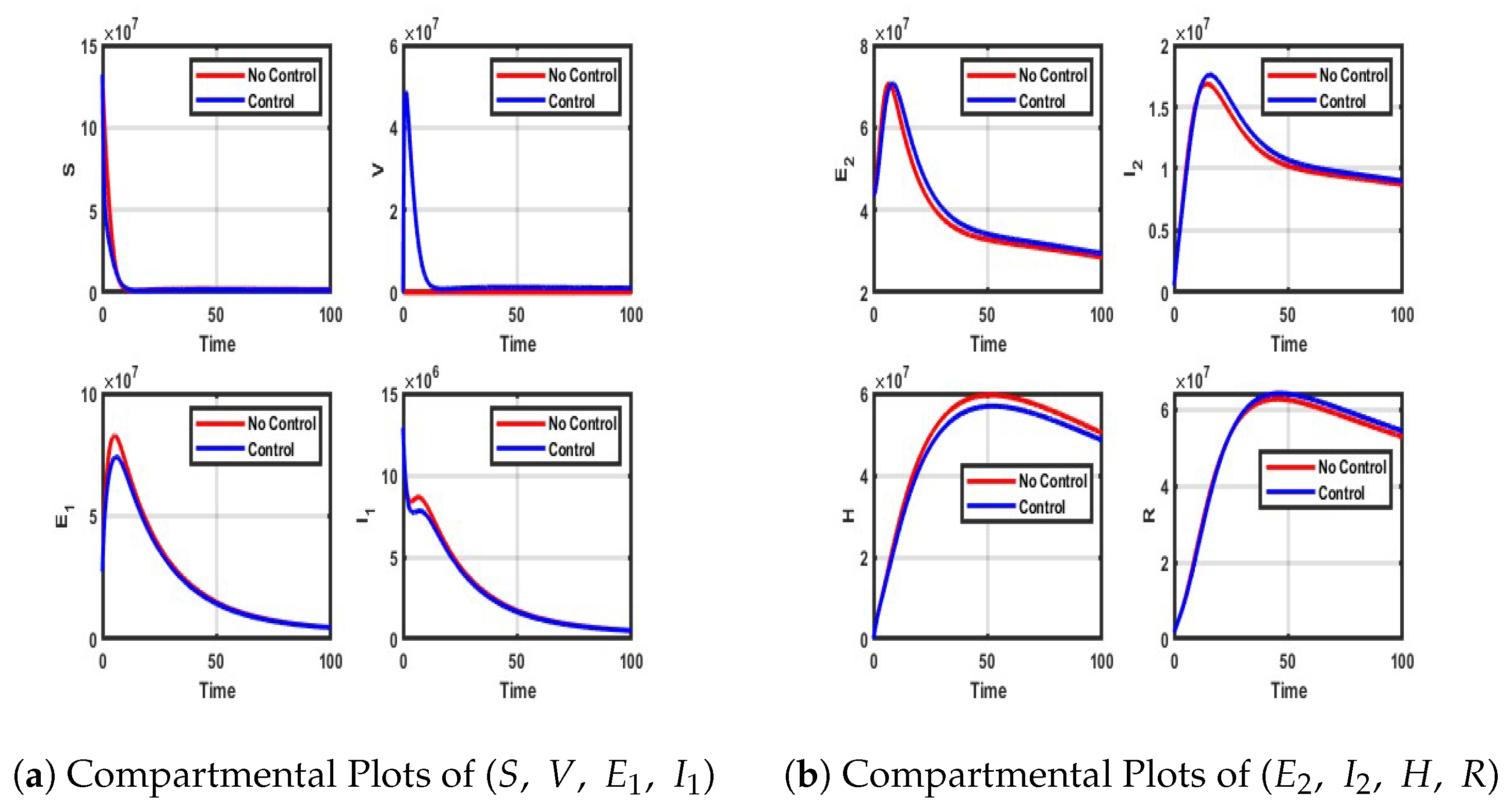
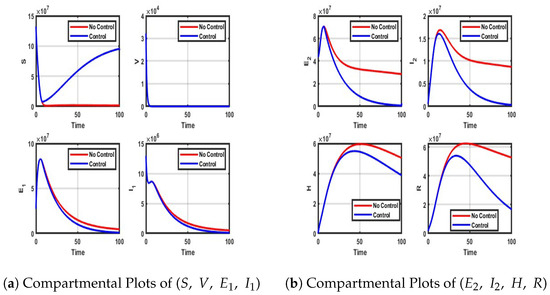
Figure A2.
Impact of Vaccination-only control on each of the model compartment.
Figure A2.
Impact of Vaccination-only control on each of the model compartment.

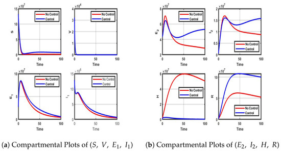
Figure A3.
Impact of Treatment only control on each of the compartment.
Figure A3.
Impact of Treatment only control on each of the compartment.

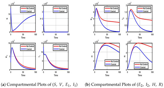
Figure A4.
Impact of vaccination and NPIs on each compartment.
Figure A4.
Impact of vaccination and NPIs on each compartment.
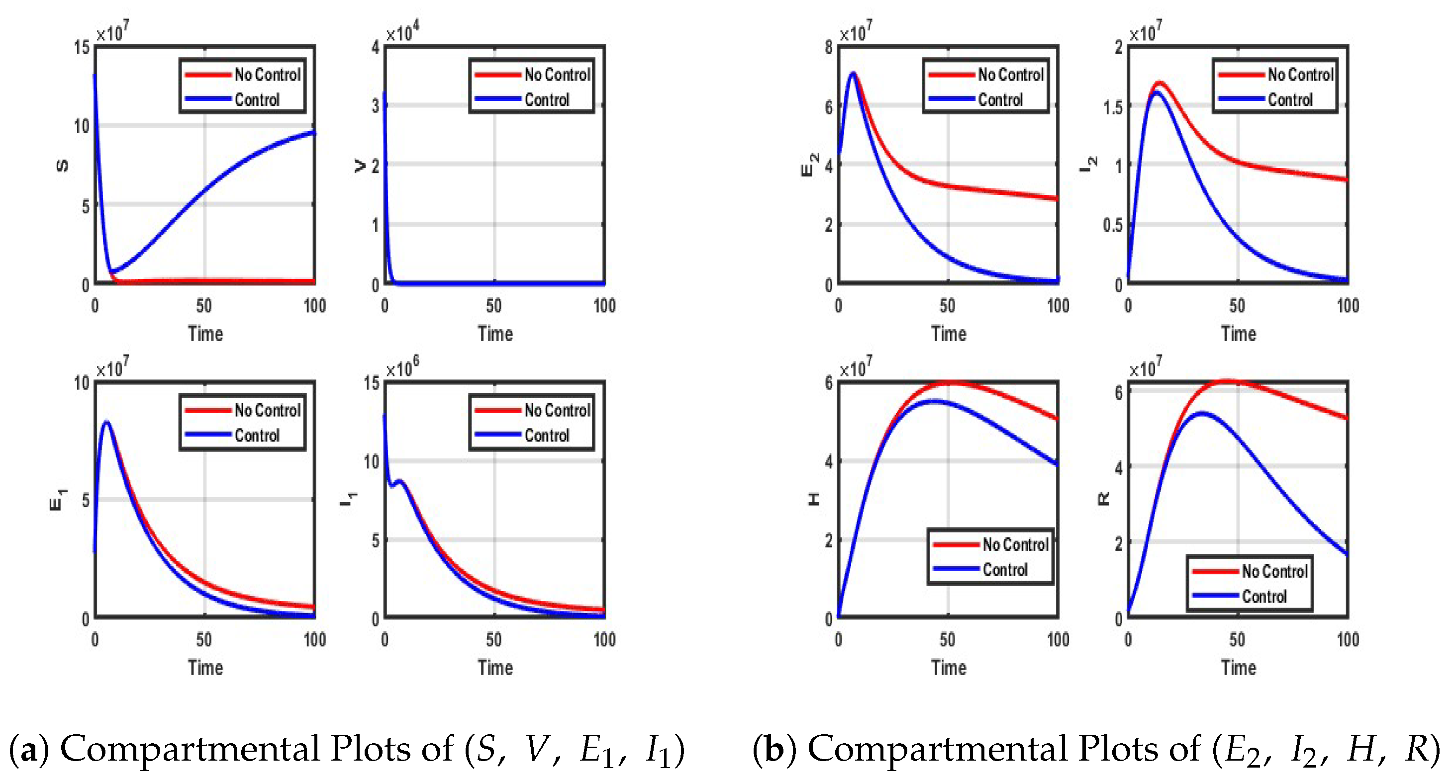
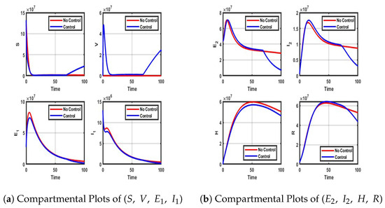
Figure A5.
Impact of NPIs and Vaccination control on each compartment.
Figure A5.
Impact of NPIs and Vaccination control on each compartment.
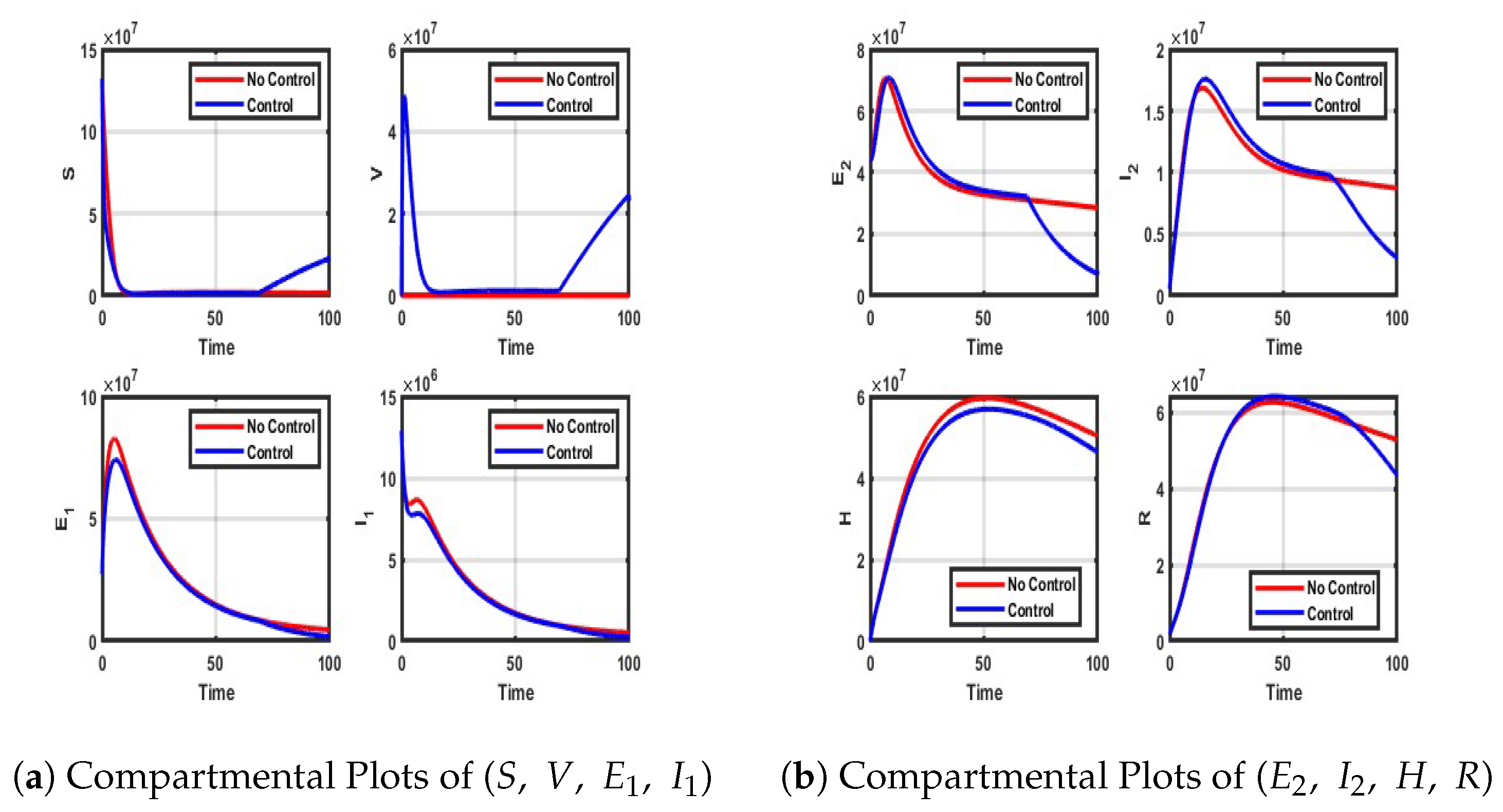
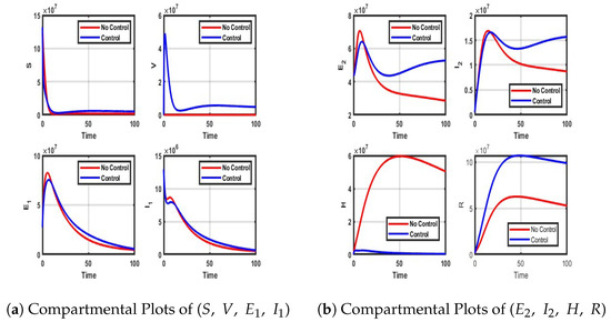
Figure A6.
Impact of Vaccination and treatment control on each compartment of the model.
Figure A6.
Impact of Vaccination and treatment control on each compartment of the model.
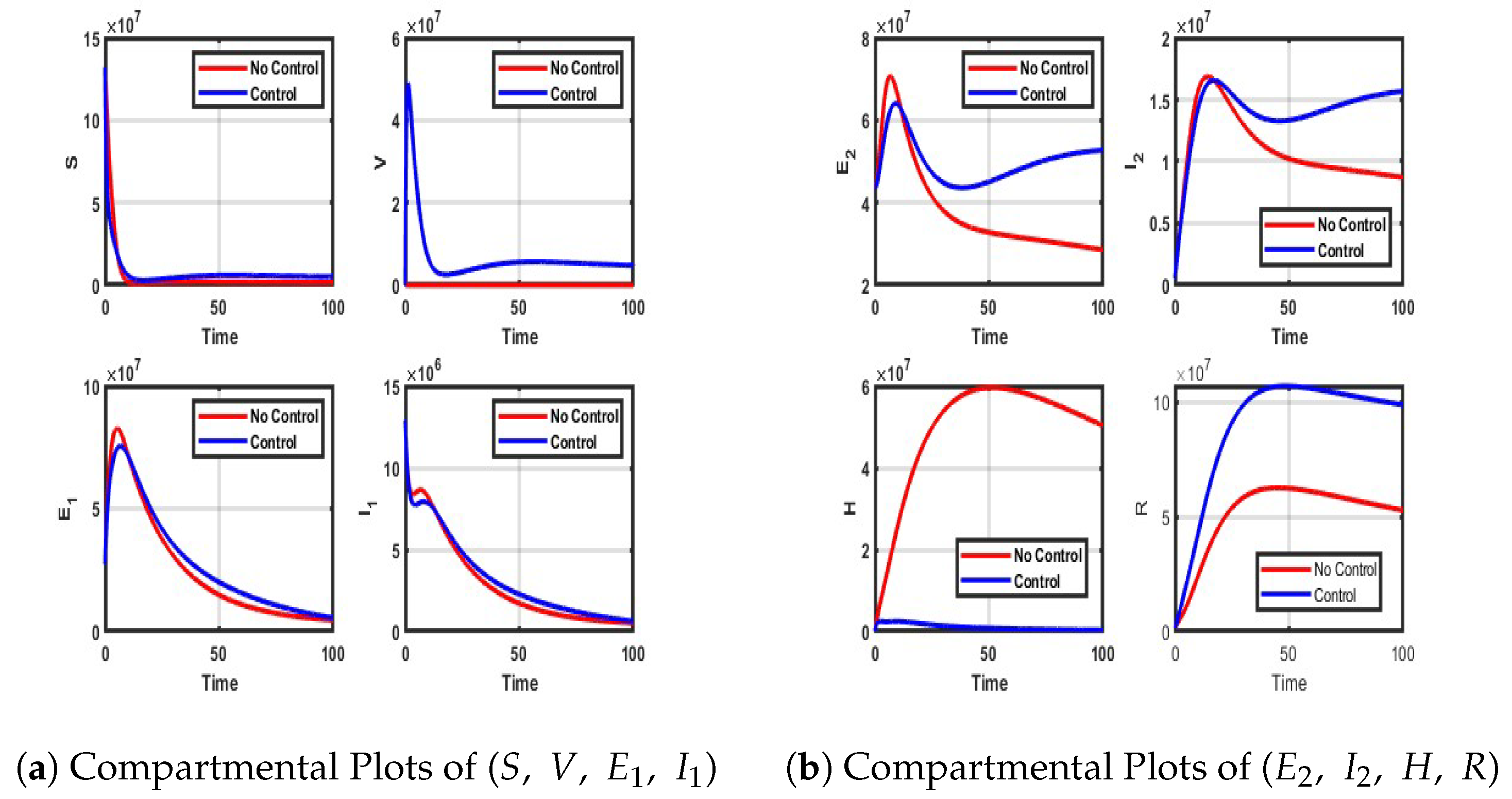
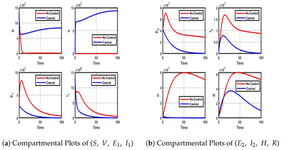
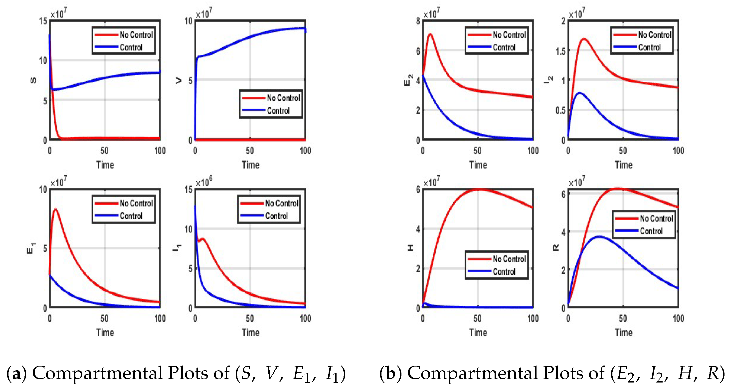
Figure A7.
Impact of vaccination, NPIs, and treatment on each compartment.
Figure A7.
Impact of vaccination, NPIs, and treatment on each compartment.
References
- Wikipedia-Optimal Control. Available online: https://en.wikipedia.org/wiki/Optimal_control (accessed on 23 January 2025).
- An Introduction to Mathematical Optimal Control Theory. Available online: https://math.berkeley.edu/~evans/control.course.pdf (accessed on 23 January 2025).
- An Introduction to Mathematical Optimal Control Theory. Available online: https://math.uchicago.edu/~may/REU2019/REUPapers/Qing.pdf (accessed on 23 January 2025).
- What Is Optimal Control Theory. Available online: https://link.springer.com/chapter/10.1007/978-3-030-91745-6_1 (accessed on 2 February 2025).
- NCBI: An Introduction to COVID-19. Available online: https://www.ncbi.nlm.nih.gov/pmc/articles/PMC7307707/ (accessed on 10 December 2024).
- WHO: Cornavirus. Available online: https://www.who.int/health-topics/coronavirus (accessed on 10 December 2024).
- Wikipedia-COVID-19. Available online: https://en.wikipedia.org/wiki/COVID-19 (accessed on 10 December 2024).
- Another New Coronavirus Variant Found in Nigeria, Says Africa CDC, Visited March 2024. Available online: https://www.reuters.com/article/us-health-coronavirus-africa-idUSKBN28Y1B7/ (accessed on 11 November 2024).
- COVID-19 Variants—What You Should Know. Available online: https://www.hopkinsmedicine.org/health/conditions-and-diseases/coronavirus/a-new-strain-of-coronavirus-what-you-should-know (accessed on 15 December 2024).
- Pérez-Lago, L.; Kestler, M.; Sola-Campoy, P.J.; Rodriguez-Grande, C.; Flores-García, R.F.; Buenestado-Serrano, S.; Herranz, M.; Alcalá, L.; Martínez-Laperche, C.; Suárez-González, J.; et al. COVID-19 superinfection and reinfection with three different strains. Transbound. Emerg. Dis. 2022, 69, 3084–3089. [Google Scholar] [CrossRef] [PubMed]
- Iboi, E.A.; Ngonghala, C.N.; Gumel, A.B. Will an imperfect vaccine curtail the SARS-CoV-2 pandemic in the US? Infect. Dis. Model. 2020, 5, 510–524. [Google Scholar] [CrossRef] [PubMed]
- Iboi, E.A.; Sharomi, O.O.; Ngonghala, C.N.; Gumel, A.B. Mathematical modeling and analysis of SARS-CoV-2 pandemic in Nigeria. MedRxiv 2020. [Google Scholar] [CrossRef]
- CDC-SARS-CoV-2 Variant Classifications and Definitions, Visited July 2023. Available online: https://www.cdc.gov/covid/?CDC_AAref_Val=https://www.cdc.gov/coronavirus/2019-ncov/variants/variant-classifications.html (accessed on 11 November 2024).
- COVID-19 Variants-Medscape-Reference. Available online: https://emedicine.medscape.com/article/2500142-overview (accessed on 15 December 2024).
- Idisi, I.O.; Yusuf, T.T.; Owolabi, K.M.; Ojokoh, B.A. A bifurcation analysis and model of SARS-CoV-2 transmission dynamics with post-vaccination infection impact. Healthc. Anal. 2023, 3, 100157. [Google Scholar] [CrossRef]
- Omorogie, E.O.; Owolabi, K.M.; Olabode, B.T. A non-linear deterministic mathematical model for investigating the population dynamics of COVID-19 in the presence of vaccination. Healthc. Anal. 2024, 5, 100328. [Google Scholar] [CrossRef]
- Omorogie, E.O.; Owolabi, K.M.; Olabode, B.T.; Yusuf, T.T.; Pindza, E. Resurgence in focus: COVID-19 dynamics and optimal control frameworks. Glob. Epidemiol. 2025, 9, 100200. [Google Scholar] [CrossRef]
- Yusuf, T.T.; Abidemi, A. Effective strategies towards eradicating the tuberculosis epidemic: An optimal control theory alternative. Healthc. Anal. 2023, 3, 100131. [Google Scholar] [CrossRef]
- Oluwasegun, M.I.; Daniel, O.; Monday, N.O. Optimal control model for criminal gang population in a limited-resource setting. Int. J. Dyn. Control 2023, 11, 835–850. [Google Scholar] [CrossRef]
- Akinyemi, S.T.; Idisi, I.O.; Rabiu, M.; Okeowo, V.I.; Iheonu, N.; Dansu, E.J.; Abah, R.T.; Mogbojuri, O.A.; Audu, A.M.; Yahaya, M.M.; et al. A tale of two countries: Optimal control and cost-effectiveness analysis of monkeypox disease in germany and nigeria. Healthc. Anal. 2023, 4, 100258. [Google Scholar] [CrossRef]
- Zakary, O.; Rachik, M.; Elmouki, I. A multi-regional epidemic model for controlling the spread of Ebola: Awareness, treatment, and travel-blocking optimal control approaches. Math. Methods Appl. Sci. 2017, 40, 1265–1279. [Google Scholar] [CrossRef]
- De la Sen, M.; Agarwal, R.P.; Nistal, R.; Alonso-Quesada, S.; Ibeas, A. A switched multicontroller for an SEIADR epidemic model with monitored equilibrium points and supervised transients and vaccination costs. Adv. Differ. Equ. 2018, 2018, 390. [Google Scholar] [CrossRef]
- Laarabi, H.; Rchik, M.; Kaddar, A. Optimal control of an epidemic model with a saturated incidence rate. Nonlin Anal. 2012, 17, 448–459. [Google Scholar] [CrossRef]
- Yusuf, T.T.; Abidemi, A.; Afolabi, A.S.; Dansu, E.J. Optimal Control of the Coronavirus Pandemic with Impacts of Implemented Control Measures. J. Nig. Soc. Phys. Sci. 2022, 4, 88–98. [Google Scholar] [CrossRef]
- Kouidere, A.; Khajji, B.; Bhih, E.A.; Balatif, O.; Rachik, M. A mathematical modeling with optimal control strategy of transmission of COVID-19 pandemic virus. Commun. Math. Biol. Neurosci. 2020, 2020, 24. [Google Scholar] [CrossRef]
- Zhong, H.S.; Yu-Ming, C.; Muhammad, A.K.; Shabbir, M.; Al-Hartomy, O.A.; Higazy, M. Mathematical modeling and optimal control of the COVID-19 dynamics. Results Phys. 2021, 31, 105028. [Google Scholar] [CrossRef]
- Omede, B.I.; Odionyenma, U.B.; Ibrahim, A.A.; Bolaji, B. Third wave of COVID-19: Mathematical model with optimal control strategy for reducing the disease burden in Nigeria. Int. J. Dynam. Control 2023, 11, 411–427. [Google Scholar] [CrossRef]
- Asamoah, J.K.K.; Zhen, J.; Sun, G.-Q.; Seidu, B.; Yankson, E.; Abidemi, A.; Oduro, F.T.; Stephen, E.M.; Okyere, E. Sensitivity assessment and optimal economic evaluation of a new COVID-19 compartmental epidemic model with control interventions. Chaos Solitons Fractals 2021, 146, 110885. [Google Scholar] [CrossRef]
- Khan, A.A.; Ullah, S.; Amin, R. Optimal control analysis of COVID-19 vaccine epidemic model: A case study. Eur. Phys. J. Plus 2022, 137, 156. [Google Scholar] [CrossRef]
- Mandal, M.; Jana, S.; Nandi, S.K.; Khatua, A.; Adak, S.; Kar, T.K. A model based study on the dynamics of COVID-19: Prediction and control. Chaos Solitons Fractals 2020, 136, 109889. [Google Scholar] [CrossRef]
- Khajji, B.; Boujalla, L.; Balatif, O.; Rachik, M. Mathematical Modelling and Optimal Control Strategies of a Multistrain COVID-19 Spread. Hindawi J. Appl. Math. 2022, 2022, 9071890. [Google Scholar] [CrossRef]
- Ahmed, E.; El Amine, B.; Hassan, L.; Abdelhadi, A.; Mostafa, R. Mathematical modeling and optimal control of multi-strain COVID-19 spread in discrete time. Front. Appl. Math. Stat. 2024, 10, 1392628. [Google Scholar] [CrossRef]
- COVID-19 Cases, 28 February 2020. Available online: https://www.worldometers.info/coronavirus/ (accessed on 10 December 2024).
- Lenhart, S.; Workman, J.T. Optimal Control Applied to Biological Models; CRC Press: Boca Raton, FL, USA, 2007. [Google Scholar]
- Koelle, K.; Martin, M.A.; Antia, R.; Lopman, B.; Dean, N.E. The changing epidemiology of SARS-CoV-2. Science 2022, 375, 1116–1121. [Google Scholar] [CrossRef] [PubMed]
- Yusuf, T.T.; Benyah, F. Optimal strategy for controlling the spread of HIV/AIDS disease: A case study of South Africa. J. Biol. Dyn. 2011, 6, 475–494. [Google Scholar] [CrossRef] [PubMed]
- Neilan, R.M.; Lenhart, S. An Introduction to Optimal Control with an Application in Disease Modeling. Am. Math. Soc. 2010, 75, 67–81. [Google Scholar] [CrossRef]
- Onifade, A.A.; Idisi, O.I.; Kareem, L.A. Modeling the transmission dynamics of COVID-19 with genetically resistant humans. Sci. Afr. 2024, 2, e02240. [Google Scholar] [CrossRef]
- Fleming, W.H.; Rishel, R.W. Deterministic and Stochastic Optimal Control; Springer: New York, NY, USA, 1975. [Google Scholar]
- Coddington, E.A.; NLevinson, N. Theory of Ordinary Differential Equations; McGraw Hill: New York, NY, USA, 1955. [Google Scholar]
- Arruda, E.F.; Das, S.S.; Dias, C.M.; Pastore, D.H. Modelling and optimal control of multi strain epidemics, with application to COVID-19. PLoS ONE 2021, 16, E0257512. [Google Scholar] [CrossRef]

Disclaimer/Publisher’s Note: The statements, opinions and data contained in all publications are solely those of the individual author(s) and contributor(s) and not of MDPI and/or the editor(s). MDPI and/or the editor(s) disclaim responsibility for any injury to people or property resulting from any ideas, methods, instructions or products referred to in the content. |
© 2025 by the authors. Licensee MDPI, Basel, Switzerland. This article is an open access article distributed under the terms and conditions of the Creative Commons Attribution (CC BY) license (https://creativecommons.org/licenses/by/4.0/).