Abstract
The article presents results of an analytical and numerical modeling of electron fluid motion and heat generation in a rectangular conductor at an alternating electric potential. The analytical solution is based on the series expansion solution (Fourier method) and double series solution (method of eigenfunction decomposition). The numerical solution is based on the lattice Boltzmann method (LBM). An analytical solution for the electric current was obtained. This enables estimating the heat generation in the conductor and determining the influence of the parameters characterizing the conductor dimensions, the parameter M (phenomenological transport time describing momentum-nonconserving collisions), the Knudsen number (mean free path for momentum-nonconserving) and the Sh number (frequency) on the heat generation rate as an electron flow passes through a conductor.
1. Introduction
In some materials, such as graphene, charge carriers interact with each other significantly, which makes it possible to consider the electron flow as a viscous fluid with properties described by Stokes’ law [1,2,3].
The mode of current carrier transfer is characterized by the transport properties of individual electrons, namely their ability to move a certain distance, after which the charged particle will collide with its own kind. This distance is usually called the electron mean free path (in graphene from l~100 nm [4] to 10 μm [3]). The mode of electron flow depends on the mean free path of the electron, the geometric dimensions of the conductor, and the presence of impurities in the conductor material [4,5,6,7].
The solution of the electron–electron transfer problem based on the Navier–Stokes equations [8] makes it possible to derive the conditions for the transition from the laminar type of electron transfer to the turbulent type in nanoscale systems. Thermal effects, the presence of a magnetic field, the relationship between charge and energy flows, and the geometry of the study sample have a significant role in the electron flow in semiconductor lattices.
At low temperatures (T = 7.5 K), the collision between electrons is suppressed and a ballistic flow regime develops [9], while an increase in temperature (T = 75 K) promotes the development of a hydrodynamic profile of electron motion.
In [9], it was found that the Hall field profile across the channel is a key physical quantity that allows one to distinguish a ballistic flow from a hydrodynamic one. The authors elucidated the transition from flat ballistic field profiles at low temperatures to parabolic field profiles at elevated temperatures, which is a distinctive feature of the Poiseuille flow.
In theoretical study [10], mathematical relations were obtained for magnetic susceptibility, longitudinal electrical conductivity, and oscillations of the electron specific heat capacity of electronic semiconductors. Analysis showed that an increase in the lattice temperature enhances the resonance peaks on the curves of the dependence of the electron drift velocity on the electric field; i.e., the speed of electron movement increases. In [11], numerical studies of the stationary transport properties of one-dimensional correlated quantum systems at zero temperature of one-dimensional correlated conductors are presented. It was shown that stationary currents can be obtained from transient currents in finite systems that are disturbed by equilibrium.
Understanding the hydrodynamic effects in an electron flow based on the generalized Navier–Stokes equations is impossible without determining the boundary conditions. In [12], a kinetic theory is developed that is based on determining the temperature dependence of the slip length at the interface for graphene and Fermi liquids. The obtained dependence of slip lengths on temperature showed a decrease in the mean free path of an electron with increasing temperature.
The problem of measuring the effect of viscosity using hydrodynamic electron transport under the influence of magnetic fields is experimentally considered in [13]. Studies enabled measuring the classical Hall viscosity of an electron gas in solid-state systems. As it is known, hydrodynamic effects in the movement of flows of various natures are closely related to heat transfer. Thermoelectric effects, the conversion of heat into electrical energy and vice versa were also intensively studied. Scientific interest in these phenomena is constantly growing due to the development of new technologies and new energy sources.
The study of new types of conductors [14,15,16,17] creates new approaches to the research of heat generation processes. The authors of [18] presented a new relation for the heat flux valid for arbitrarily high frequencies, which also describes the processes of tunneling with the participation of photons in heat transfer. This relation is most preferable for low excitation amplitudes, which made it possible to determine the property of electrothermal conductivity to change its sign.
In [19], the electron–phonon interaction and its effect on charge and energy transfer were studied. The possibility of calculating the Joule heating current, at the nanoscale, for processes when the heat dissipated by electrons is transferred to and from the nanoconductor was shown.
Heat transfer from electrons to acoustic and optical phonons in monolayer and bilayer graphene was calculated in [20]. Cases at very low temperatures were studied where acoustic coupling with phonons in the sample affects Joule heating. Also, cases with higher temperatures, when optical phonons begin to dominate, were explored as well.
The lattice Boltzmann method (LBM) is a class of computational hydrodynamic solutions that models flow using a discrete kinetic Boltzmann equation. The LBM offers an efficient and accurate algorithm for solving hydrodynamics problems of viscous electron fluids since viscosity is naturally included in its formulation. In [2], the authors developed an oscillating flow model of femtofluid in flat and cylindrical conductors. Analytical data were compared with numerical results obtained using LBM, showing good agreement. The influence of dimensionless parameters Sh, Fo, and Kn on femtofluid behavior was shown. The skin effect and current density reduction with increasing oscillation frequency were explained.
Recent studies have shown that certain characteristics of electron flow in graphene (in particular, the formation of hydro-electronic vortices) can be described using the relativistic lattice Boltzmann method [21]. The results confirm earlier theoretical and experimental findings.
Given the above, it can be said that the research on the behavior of electron fluids is highly relevant. However, most works focus on the hydrodynamics of the flow.
The purpose of this article is to investigate the flow of charge carriers and analyze the heat release process in rectangular conductors. Since the LBM has shown the adequacy of the obtained results [22,23,24,25,26], in this work, the analytical results are compared with numerical ones using LBM. In paper [27], an attempt was made for the first time to develop an analytical research method which is based on the Lie symmetry group approach for calculating the electron fluid flow around a spherical barrier in a three-dimensional formulation. Thus, the objective of this work is to study the movement of charge carriers in a rectangular conductor under the influence of an alternating electric field. The results obtained will help to understand the processes occurring in real conductors and will help to design new electronic devices with improved characteristics.
2. Governing Equations
Let us consider the unsteady flow of electron fluid through rectangular conductors with length l, width 2h, and height 2b (Figure 1). The electrical potential φ is applied to the conductor. The origin of the coordinate system is located in the center of the conductor. Axis z is the longitudinal coordinate, while axis y and x determine the height and width, respectively.
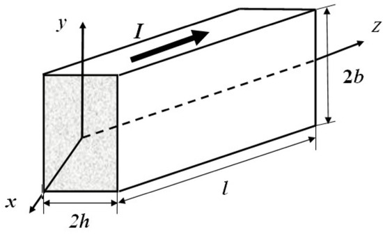
Figure 1.
Schematic representation of the problem.
A modified Navier–Stocks equation is used to describe the electronic fluid flow in the geometry in Figure 1 [2]
where is the streamwise (longitudinal) velocity, e is the electron charge, m is the electron effective mass, τ is the phenomenological transport time describing momentum-nonconserving collisions, e is the electron charge, m is the electron effective mass, ν is the kinematic viscosity, and φ is the electrostatic potential.
The first term on the right-hand side of Equation (1) takes into account the electric force expressed through the electric potential, while the second term stands for the effect of shear viscosity expressed through the kinematic viscosity ν. The third term includes the time between carrier collisions τ describing the dissipation of momentum during the scattering of current carriers on impurities and phonons.
Equation (1) must be solved under the follow boundary conditions
where L is the mean free path for momentum-nonconserving collisions, b is half of the channel height in the z direction, and the origination point of the z axis is in the center of the channel (Figure 1).
Alternating electric potential is described as
where ω is the frequency of oscillations.
The solution of Equation (1) has the following form
The substitution of Equations (6) and (7) into Equation (1) gives
The dimensionless form of Equation (8) is
where
The solution of Equation (9) requires nondimensionalizing of the boundary conditions
where
is the Knudsen number for electron fluid. The Knudsen number is a dimensionless mean free path of momentum-nonconserving collisions, so this parameter also takes into account impurities on the walls of the channel.
3. Series Solution (Fourier Method)
Let us present the solution of Equation (8) in the series form
Then, it is necessary to consider the homogenous operator of the non-homogenous Equation (9)
The substitution of the series expansion (17) into operator (18) yields
Performing the separation of variables, one can obtain
where is the separation constant, which should be found from the boundary conditions. One can derive from Equation (20)
This equation has a simple trigonometric solution
Using the boundary conditions (10) and (11), one can find
Because of the profile symmetry with respect to the center line of the channel, one can obtain = 0. As a result, one can derive a transcendent equation for the determination of the separation constant
Then, let us substitute Equation (17) into Equation (9) with account for Equation (21). This yields
Here, we use the decomposition of unity on the basis of the functions , where represents the unknown coefficients. Therefore, we have an equation for the functions
The solution of this equation under the boundary condition (13) and (14) is
Using the orthogonal properties of the basic function , let us find out the unknown coefficients from Equation (24)
The substitution of Equations (22), (28) and (29) into series expansion (17) yields the velocity distribution
To extract the real and imaginary parts from Equation (30), we will remove the radicals of complex numbers. To achieve this, we use the equation
Then, we multiply and divide the fractions in Equation (30) by the complex conjugates of the denominators of the fractions in Equation (30). As a result, we can extract real and imaginary parts.
Let us substitute Equation (30) with account of Equation (31) into Equation (7). As a result, one can obtain the velocity profile
Ther average velocity for the single oscillation period is
Then, the electrical current is expressed as follows
where
Next, taking into account Equation (34), we can find the specific current density
where is the conductor cross-sectional area.
From Equation (36), one can determine the static conductivity, which is the coefficient of proportionality between the density of the resulting current and the magnitude of gradient of electrostatic potential
where n is the steady-state charge distribution.
For a flat conductor, Equation (37) reduces to
Consequently, shear viscosity can be calculated as [22]
where is a finite value of the shear modulus, is the “viscosity transport time”, represents the high-frequency shear viscosities, and ω0 is the frequency of the external perturbation.
Let us find the current averaged over the oscillation period in relative form using Ohm’s law. According to Ohm’s law, the current through the conductor is determined as
where is the resistance of the conductor, is the voltage measured across the conductor, l is the length of the conductor, and S is the cross-sectional area of conductor.
It is known that the intensity of heat release q is proportional to the product of the square of the current and the resistance of the conductor. Considering Equations (34), (37) and (40), one can obtain
The heat release intensity can vary widely and depends mostly on the velocity and viscosity of the flow. In laminar flow, heat release is determined by the dependence . Calculations for the flow of electronic fluid showed that heat release is determined as
4. Double Series Solution (Method of Eigenfunction Decomposition)
In this method, the double series is used to present the solution in the following form
where represents the coefficients, which are unknown so far, while and are the eigenfunctions of the homogenous operator (18). The functions satisfy Equation (21) and have the form given by Equation (22) with = 0. The eigenvalues satisfy the transcendental Equation (25). The functions can be found from the similar equation
The solution of Equation (44) is
Using the boundary conditions (11)–(14), one can find
Because of the profile symmetry with respect to the centerline of the channel, one can obtain = 0. As a result, one can derive a transcendent equation for the determination of the separation constant
Let us use a decomposition of on the basis of the functions and
Based on the orthogonal properties of the basic functions and , we have from Equation (49)
The next step is the determination of the coefficient in the series (43). For this purpose, let us substitute series (43) into the left-hand side of Equation (8) and substitute series (49) into the right-hand side of Equation (8). As a result, one can obtain
Thus, the velocity distribution can be presented as
After repeating the entire procedure outlined in Section 3, one can obtain an expression for the electric current in the conductor
The calculations performed below showed complete agreement between the results for the series solution and double series solution methods.
5. Results and Discussion
In addition to analytical calculations, numerical simulations of the carrier transport hydrodynamics were performed using the LBM [24,28,29]. The Palabos library on a D3Q27 lattice was used for the simulations. The last term in Equation (1) was considered as an external force following the methodology of [26]. The velocity scale was adjusted so that the speed of light was equal to unity [30].
Electrical potential is defined as
where is the amplitude.
While investigating the influence of grid sizes, the results were compared for grids 40 × 40 × 300, 60 × 60 × 400 and 80 × 80 × 500. The difference in the estimates for grids 60 × 60 × 400 and 80 × 80 × 500 did not exceed 0.07%. Therefore, a grid with cell divisions of 60 × 60 × 400 along the x, y and z axes, respectively, was used for the calculations.
The velocity profiles were normalized by the velocity value at the center of the conductor
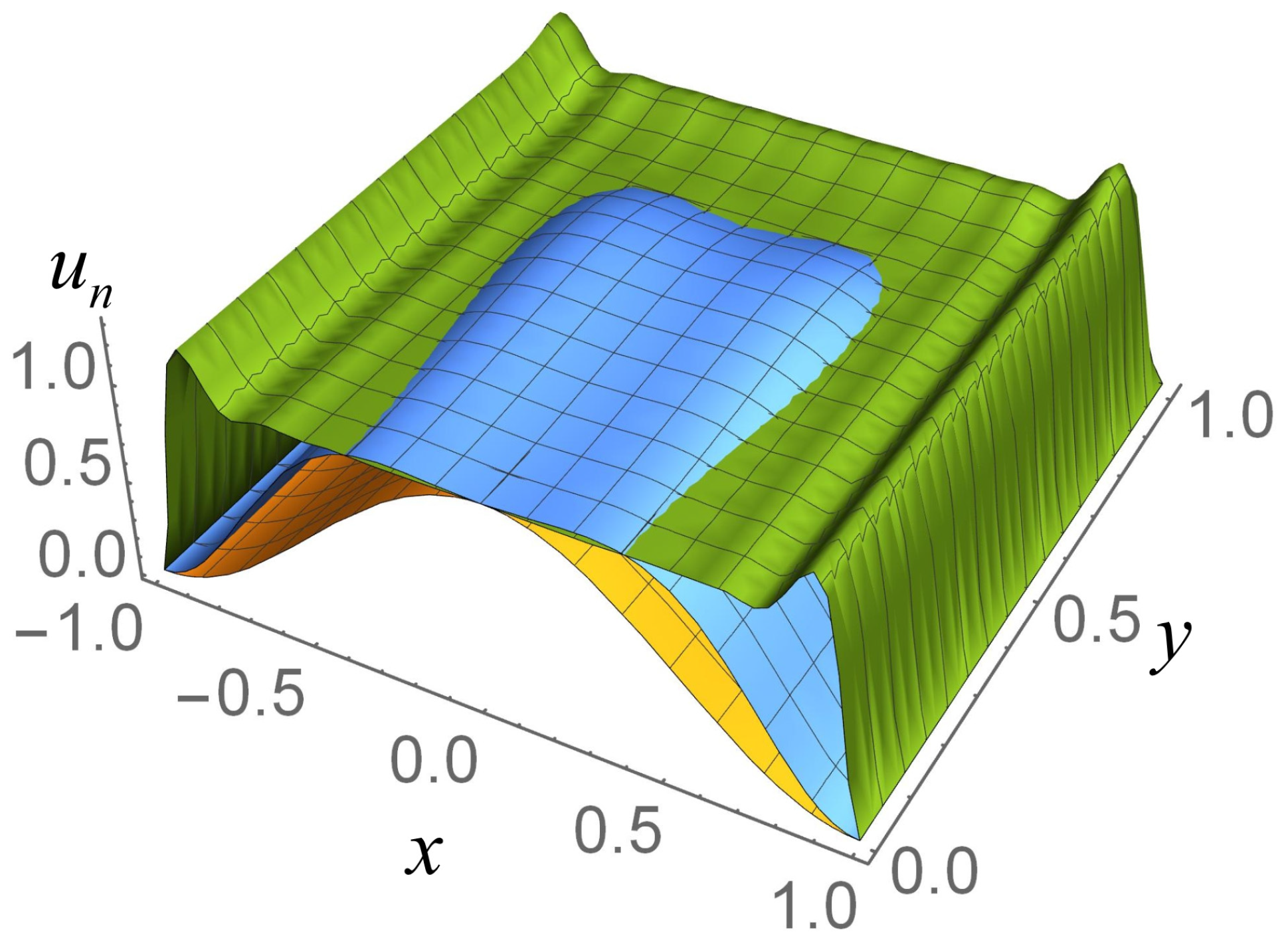
Figure 2 shows a three-dimensional profile of the averaged velocity un of charge carriers defined as Equation (33) and normalized in the form of Equation (55) in a rectangular conductor for different values of the Strouhal number Sh. Half of the profile cut by the plane y = 0 is shown.

Figure 2.
Profiles of normalized velocity un in a rectangular conductor for different values of the parameter Sh. Kn = 0.0, yellow—Sh = 1; blue—Sh = 6; green—Sh = 30.
Figure 2 demonstrates that an increase in the oscillation frequency (the Strouhal number, according to Equation (1), is proportional to the oscillation frequency of the electric field) leads to a transition from the hydrodynamic mode of charge carrier motion to the ballistic mode (the profile filling increases). Then, with an increase in frequency, the maximum carrier flow shifts toward the conductor surface. This tendency in the behavior of charge carriers is explained by the skin effect [31], when in a conductor at a high frequency of alternating voltage, the maximum current is observed near the conductor surface. Calculations show that transition to a ballistic regime occurs after Sh = 6.
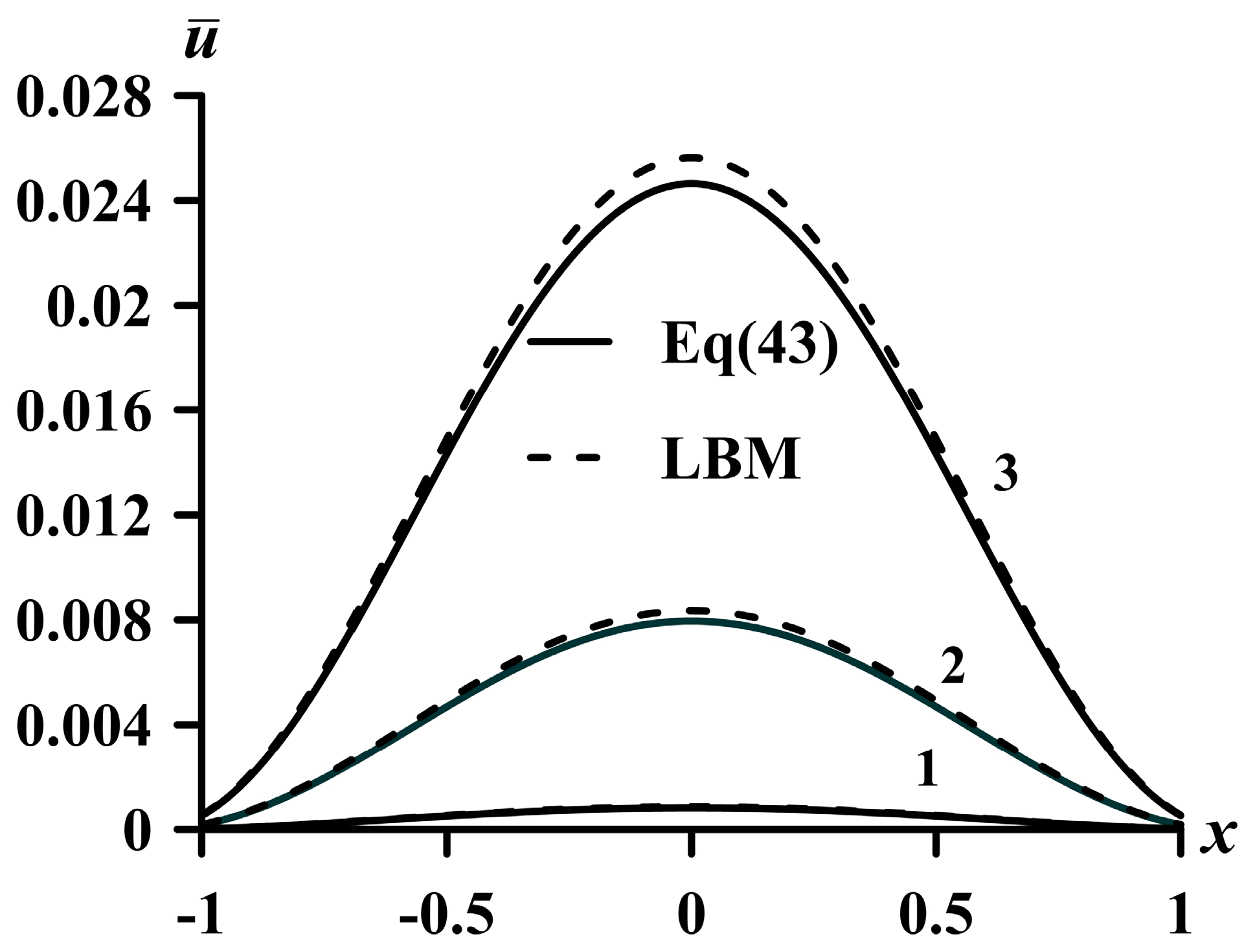
The effect of the parameter M on the behavior of the carrier velocity profiles in the electron fluid averaged over the oscillation period is shown in Figure 3. Solid lines are analytical profiles plotted based on Equation (33), and dotted lines are numerical results of the LBM. The maximum difference between analytical and numerical results did not exceed 5%.
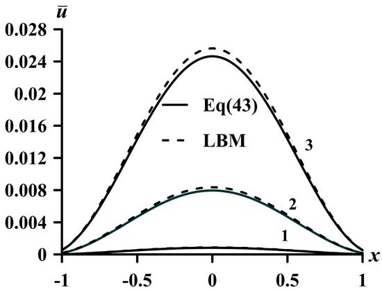
Figure 3.
Transverse profiles of the carrier velocity averaged over the period for different values of the parameter M: (1) M = 0; (2) M = 1; (3) M = 2.
Figure 3 shows that increasing the value of the parameter M increases the value of the maximum velocity. This behavior is explained by the fact that the parameter M, according to Equation (10), is proportional to τ (the time between collisions). An increase in time reduces the impact of collisions on the velocity profiles and leads to a decrease in resistance. And, therefore, the maximum value of the velocity profile increases.
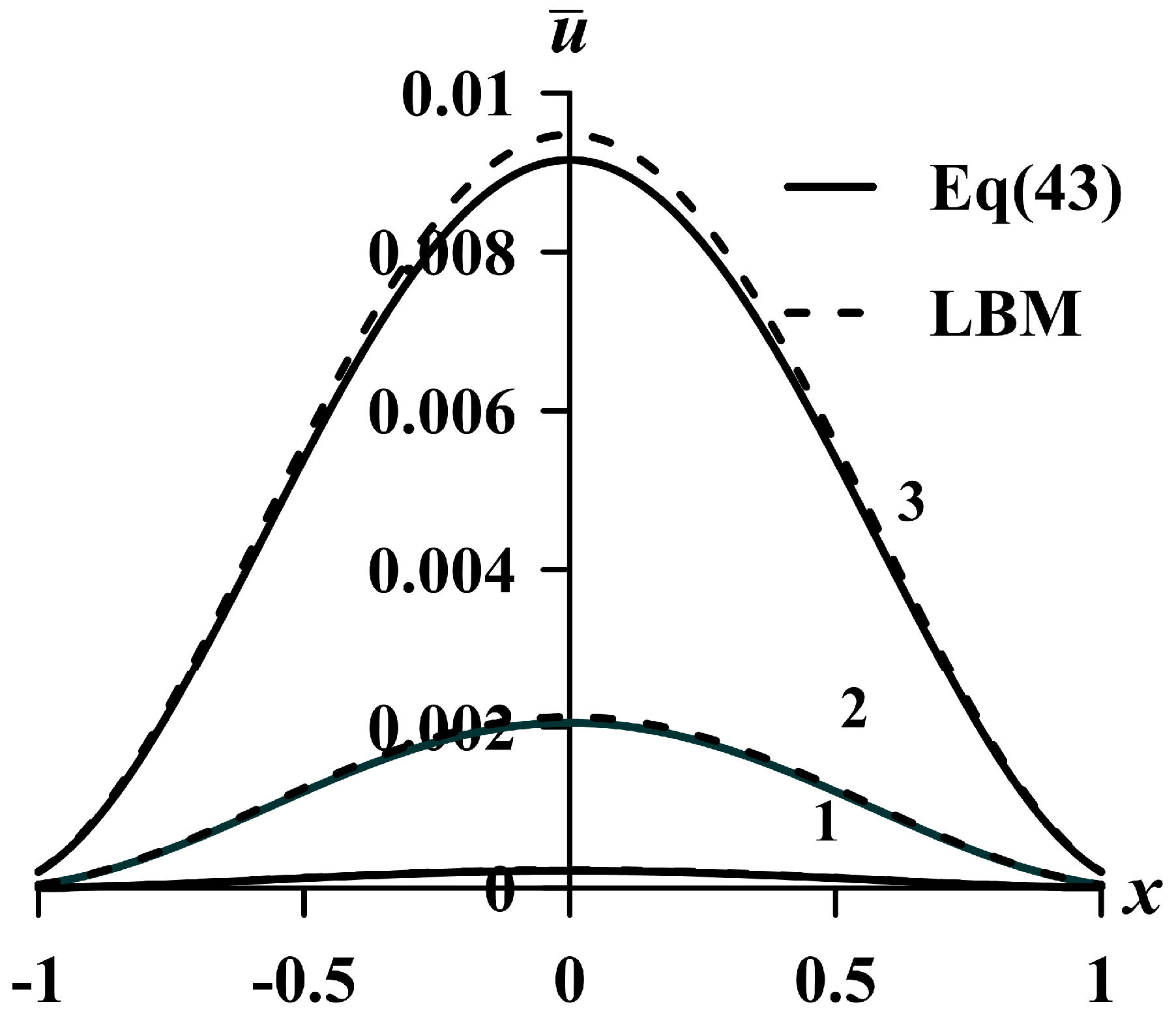
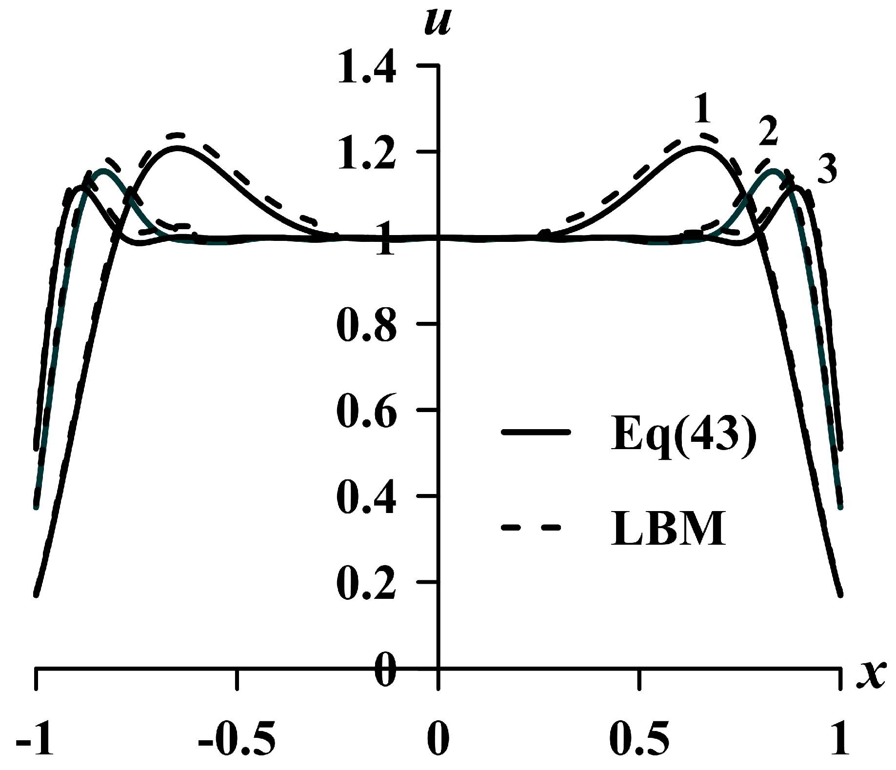
The effect of the parameter Sh on the behavior of the velocity profiles averaged over the oscillation period in the electron fluid is shown in Figure 4, Figure 5 and Figure 6.
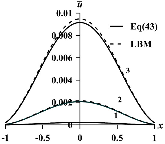
Figure 4.
Velocity profiles for Kn = 0.1 and different values of Sh number. (1) Sh = 0.001; (2) Sh = 2; (3) Sh = 3.
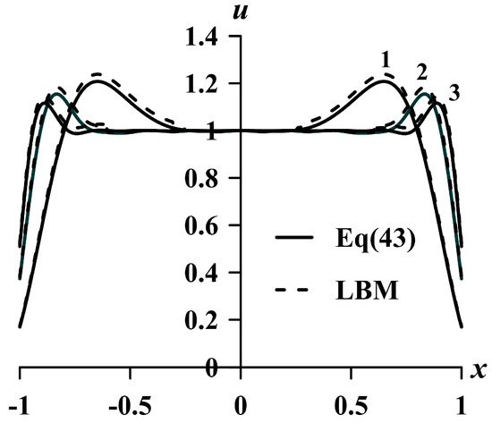
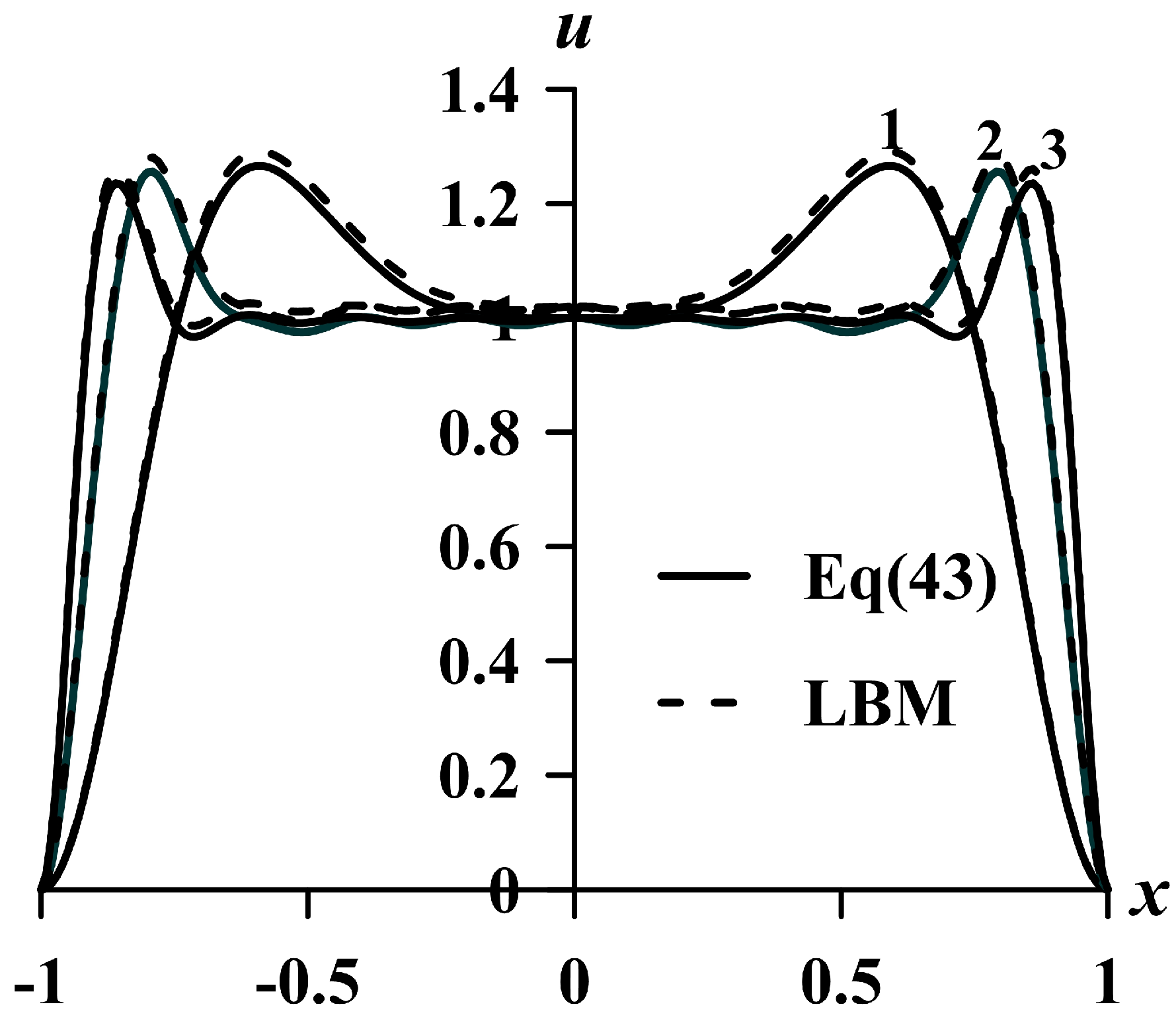
Figure 5.
Velocity profiles for Kn = 0.1 and different values of Sh number. (1) Sh = 10; (2) Sh = 20; (3) Sh = 30.
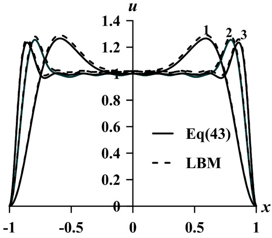
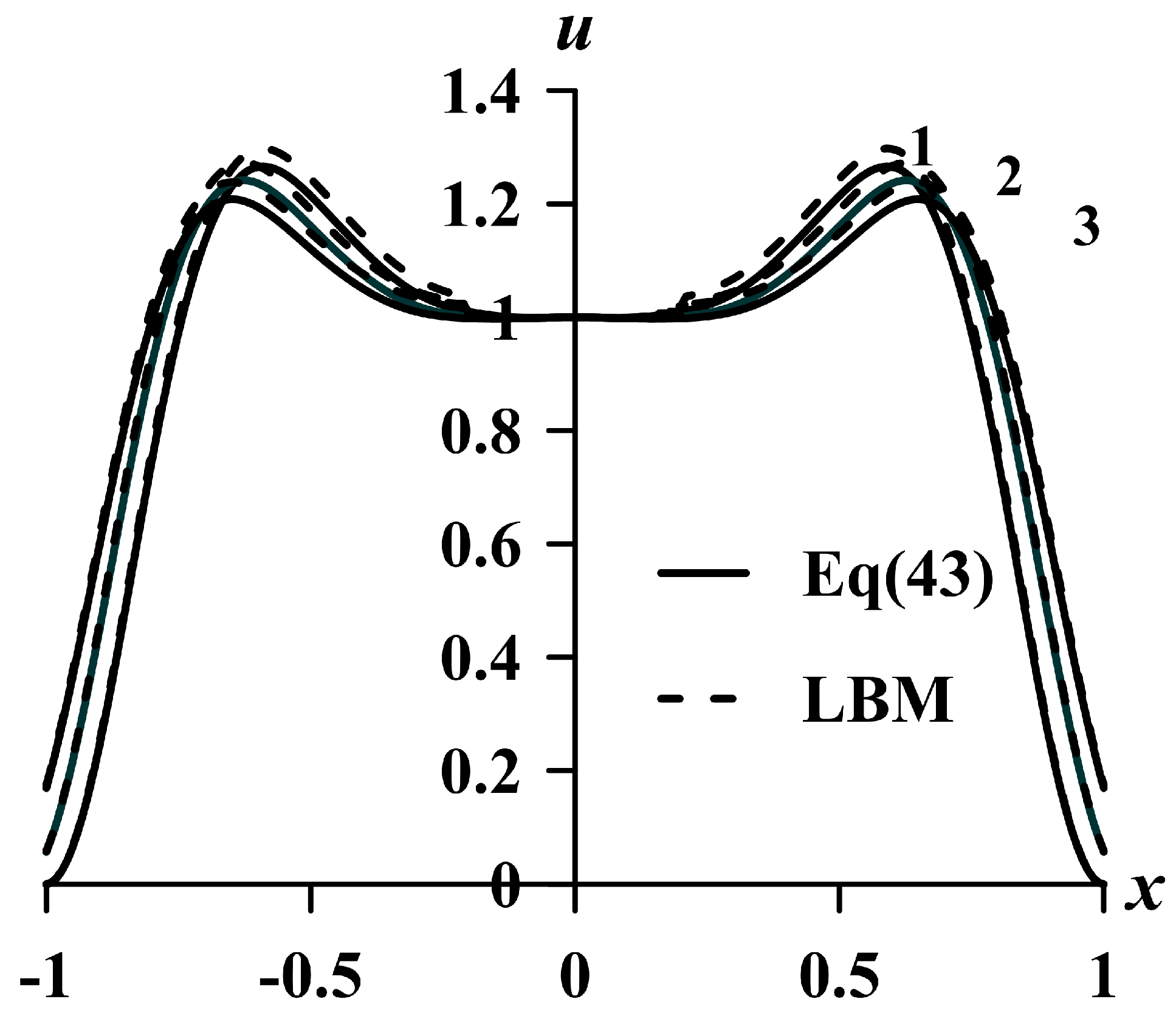
Figure 6.
Velocity profiles for Kn = 0.001 and different values of Sh number. (1) Sh = 10; (2) Sh = 20; (3) Sh = 30.
Figure 7 elucidates the influence of Knudsen number on the velocity profile. Increasing the Knudsen number results in higher velocities closer to walls of the channel, while it does not affect the velocity in the center of the channel (for Sh = 10).
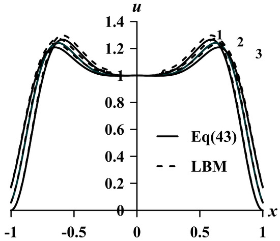
Figure 7.
Velocity profiles for Sh = 10 and different values of Kn number. (1) Kn = 0.001; (2) Kn = 0.05; (3) Kn = 0.1.
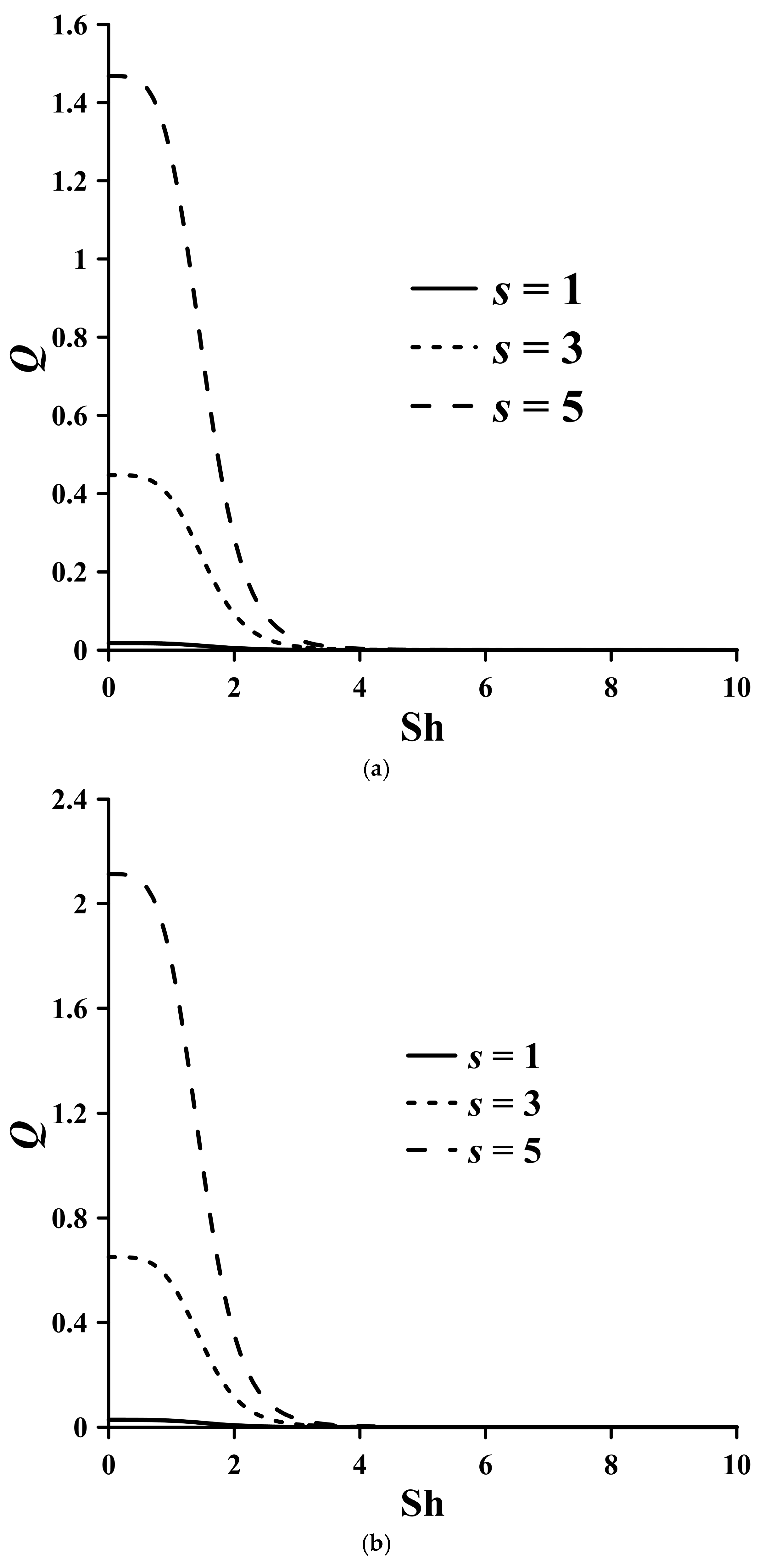
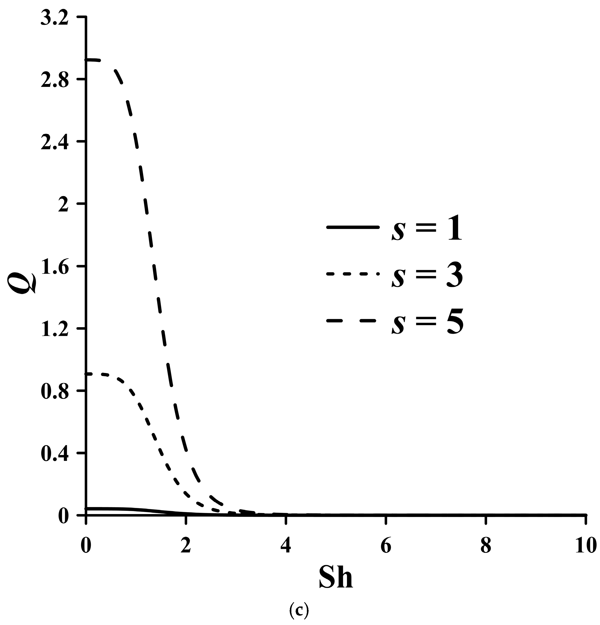
The process of heat generation in conductor materials is associated with the influence of several parameters. As mathematical transformations demonstrated, they include a parameter that characterizes the geometric size of the conductor (s), which affects the mean free path of electrons (Kn). Parameter M is inversely proportional to the electron scattering time τ and describes the effect of electron momentum nonconserving collisions and a parameter that takes into account the variability of the current, namely oscillatory effects (Sh). The results of calculating heat generation based on the Fourier series method (Figure 8, Figure 9 and Figure 10) show that an increase in oscillatory effects (Sh) leads to a decrease in heat generation. An increase in parameter s indicates a decrease in the intensity of electron collisions, which reduces resistance. As a result, the speed of the so-called electron fluid increases and, accordingly, heat generation in the conductor increases (Figure 8).
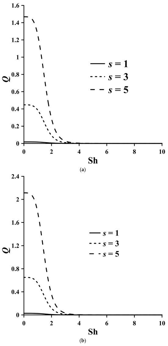
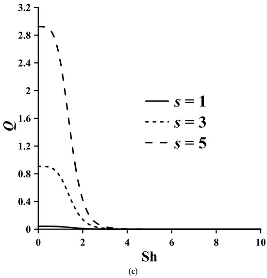
Figure 8.
Effect of the Sh number and parameter s on the amount of heat release at (a) Kn = 0.001, (b) Kn = 0.05, (c) Kn = 0.1.
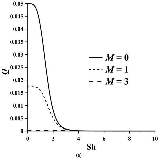

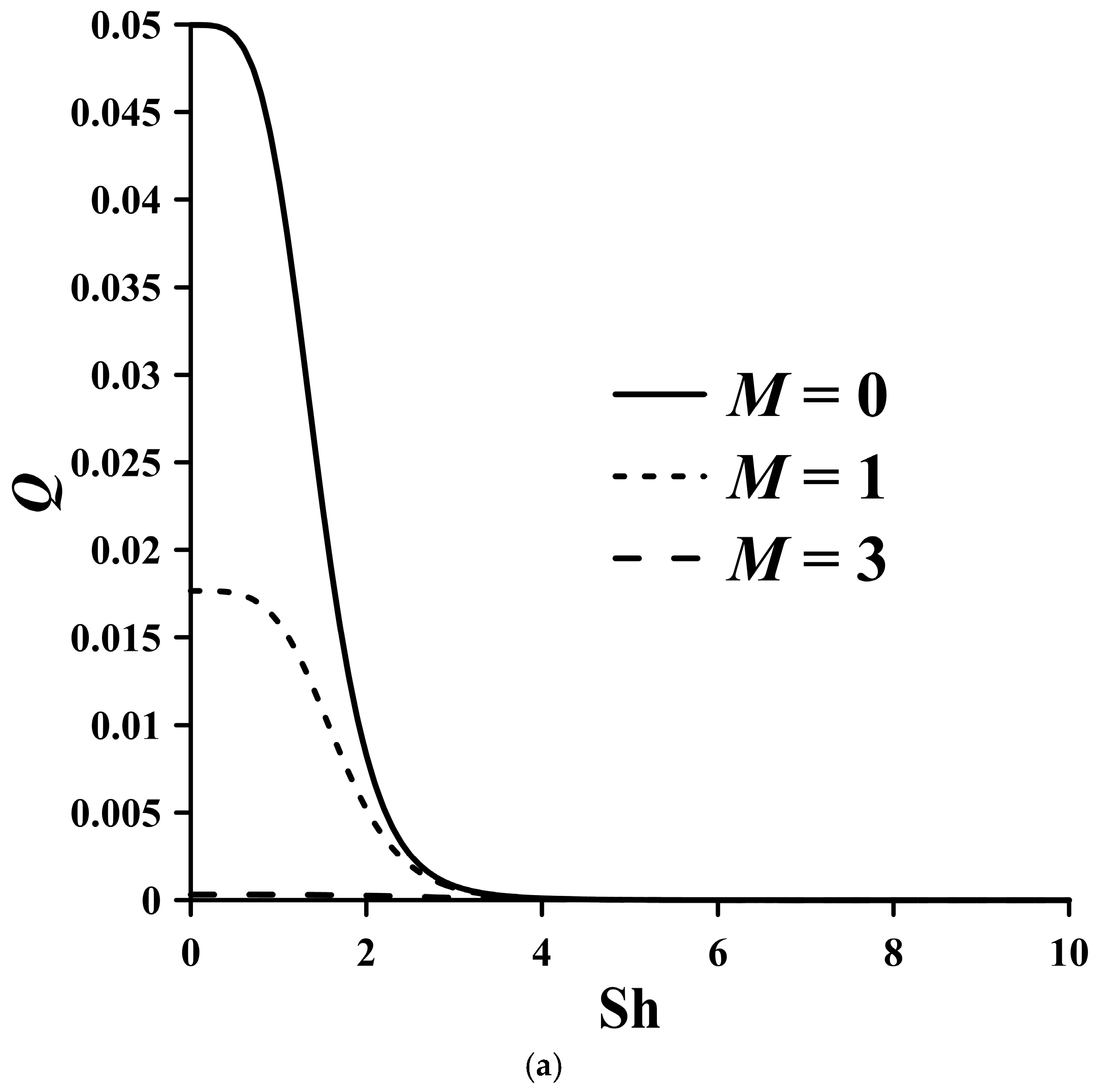
Figure 9.
Effect of the Sh number and parameter M on the amount of heat release at (a) Kn = 0.001, (b) Kn = 0.05, (c) Kn = 0.1.

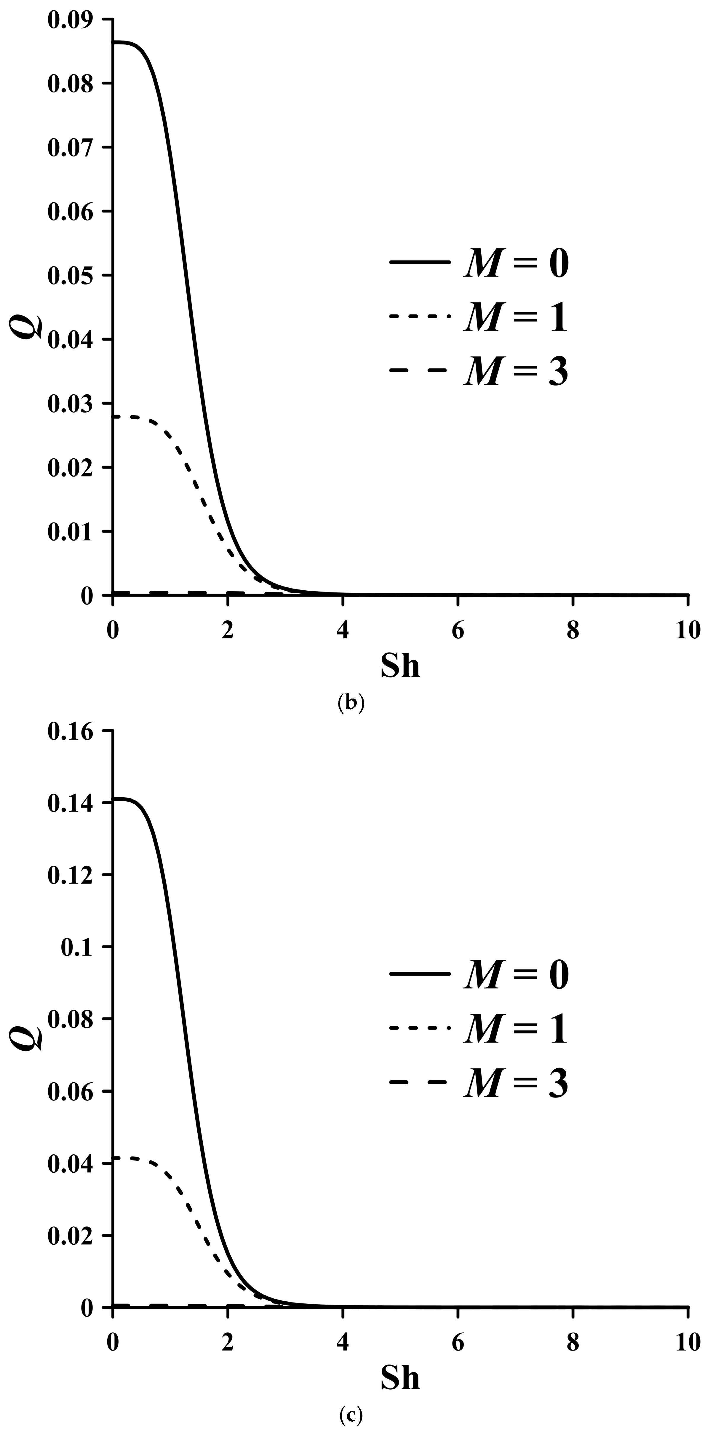
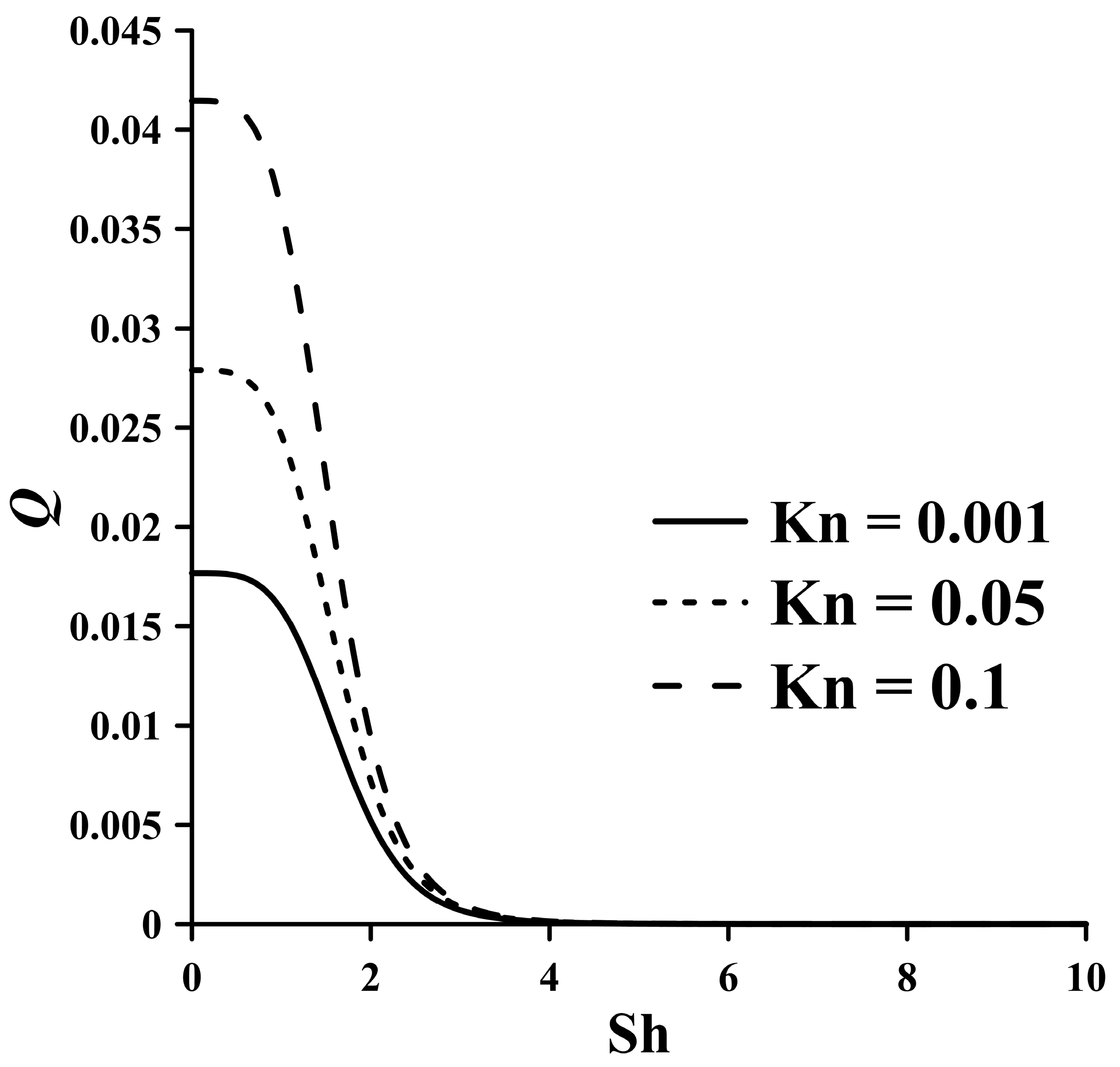
Figure 10.
Effect of the Sh and Kn numbers on the amount of heat release at M = 1, s = 1.
An increase in parameter M leads to a decrease in heat generation at smaller values of Sh number (Figure 9), which can be explained by the decrease in relaxation time.
At small values of Sh, an increase in slip effects (Kn) gives an increase in heat generation due to an increase in the velocity on the surface of the conductor, since an increase in the mean free path L improves conductivity (Figure 10).
6. Conclusions
An unsteady model of femtofluid flow in flat and cylindrical conductors has been developed. The model is based on the similarity of behavior of charge carriers of a conductor and liquids. An analytical solution of the profiles of velocity and current was obtained based on Laplace transforms. The analytical data were compared with the numerical results obtained using LBM. The difference between analytical and numerical solutions did not exceed 5%.
It is shown that the behavior of femtofluid under the influence of an oscillating potential gradient is determined by three dimensionless parameters: M, s, Sh, and Kn.
With increasing frequency (Sh) in flat and circular conductors, the maximum of the particle flux averaged over the oscillation period shifts from the center to the periphery. This trend in profile behavior is explained by the skin effect.
A comparison of the profiles in Figure 7 shows the effect of the mean free path for momentum-nonconserving collisions. An increase in the mean free path for momentum-nonconserving collisions (Kn) leads to an increase in the speed on the surface of the conductor. This effect increases with increasing frequency. Increasing the Knudsen number enhances heat generation at lower Sh number values due to the greater average speed of the charge carriers.
An increase in L (Kn) leads to a decrease in the number of collisions and, consequently, to a decrease in the resistance of the conductor and an increase in the density of the current. As the frequency increases, this effect decreases due to the formation of vortices when the polarity changes. The results obtained by analytical and numerical modeling are in good agreement.
An increase in the frequency of oscillation leads to a decrease in current density due to there being an increase in the inductive reactance of the conductor.
As the frequency increases, the randomness of the movement of carriers and the number of their collisions increases, which also leads to an increase in resistance, which results in there being a decrease in heat generation.
Increasing the M parameter (decreasing the effect of carrier collisions) leads to an increase in current density. As the frequency increases, the effect of the M parameter decreases due to the formation of vortices. At lower Sh values, any increase in parameter M reduces heat generation due to the decreased relaxation time. An increase in parameter s decreases the intensity of charge carrier collisions, which reduces resistance. As a result, heat generation in the conductor increases.
It is shown that unlike classical hydrodynamics, when the heat flow is proportional to the value of , for electron fluids, the heat flow is proportional to .
Author Contributions
Conceptualization, A.A.A. and I.V.S.; Methodology, Y.Y.K., I.V.S., N.P.D. and A.I.T.; Software, Y.Y.K., N.P.D., A.I.T. and A.S.K.; Validation, A.I.T.; Formal analysis, Y.Y.K., A.A.A. and I.V.S.; Investigation, A.A.A. and I.V.S.; Data curation, Y.Y.K. and A.S.K.; Writing—original draft preparation, Y.Y.K., A.A.A., I.V.S., N.P.D. and A.I.T.; Writing—review & editing, Y.Y.K., A.A.A., I.V.S., N.P.D. and A.S.K.; Visualization, A.A.A. All authors have read and agreed to the published version of the manuscript.
Funding
The research contributions of the authors A.A.A., N.P.D., A.I.T., Y.Y.K. and A.S.K. were funded in frames of the program of research projects of the National Academy of Sciences of Ukraine (No. 6541230), “Support of priority for the state scientific researches and scientific and technical (experimental) developments” 2025–2027 (1230), Project: “Development of distributed energy based on the use of gas turbine and gas piston technologies and local alternative fuels during the period of martial law and the restoration of Ukraine”.
Data Availability Statement
The original contributions presented in this study are included in the article. Further inquiries can be directed to the corresponding author.
Conflicts of Interest
The authors declare no conflict of interest.
References
- Bandurin, D.A.; Torre, I.; Kumar, R.K.; Shalom, M.B.; Tomadin, A.; Principi, A.; Auton, G.; Khestanova, E.; Novoselov, K.S.; Grigorieva, I.V.; et al. Negative local resistance caused by viscous electron backflow in graphene. Science 2015, 351, 1055–1058. [Google Scholar] [CrossRef]
- Avramenko, A.A.; Tyrinov, A.I.; Kovetska, Y.Y.; Konyk, A. Oscillating flow of viscous electron fluids. Chin. J. Phys. 2024, 87, 635–645. [Google Scholar] [CrossRef]
- Polini, M.; Geim, A.K. Viscous electron fluids. Phys. Today 2020, 73, 28–34. [Google Scholar] [CrossRef]
- Lucas, A.; Fong, K.C. Hydrodynamics of electrons in graphene. J. Phys. Condens. Matter 2018, 30, 053001. [Google Scholar] [CrossRef]
- Jong, M.D.; Molenkamp, L.W. Hydrodynamic electron flow in high-mobility wires. Phys. Rev. B 1994, 51, 13389–13402. [Google Scholar] [CrossRef]
- Ahn, S.; Das Sarma, S. Hydrodynamics, viscous electron fluid, and Wiedemann-Franz law in two-dimensional semiconductors. Phys. Rev. B 2022, 106, L081303. [Google Scholar] [CrossRef]
- Makhviladze, T.M.; Sarychev, M.E. Influence of point defects on the initiation of electromigration in an impurity conductor. Russ. Microelectron. 2021, 50, 339–346. [Google Scholar] [CrossRef]
- D’Agosta, R.; Di Ventra, M. Hydrodynamic approach to transport and turbulence in nanoscale conductors. J. Phys. Condens. Matter 2006, 18, 11059–11065. [Google Scholar] [CrossRef]
- Sulpizio, J.A.; Ella, L.; Rozen, A.; Birkbeck, J.; Perello, D.J.; Dutta, D.; Ben-Shalom, M.; Taniguchi, T.; Watanabe, K.; Holder, T.; et al. Visualizing Poiseuille flow of hydrodynamic electrons. Nature 2019, 576, 75–79. [Google Scholar] [CrossRef]
- Gulyamov, G.; Erkaboev, U.I.; Rakhimov, R.G.; Mirzaev, J.I. On temperature dependence of longitudinal electrical conductivity oscillations in narrow-gap electronic semiconductors. J. Nano-Electron. Phys. 2020, 12, 03012. [Google Scholar] [CrossRef]
- Einhellinger, M.; Cojuhovschi, A.; Jeckelmann, E. Numerical method for nonlinear steady-state transport in one-dimensional correlated conductors. Phys. Rev. B 2012, 85, 235141. [Google Scholar] [CrossRef]
- Kiselev, E.I.; Schmalian, J. The boundary conditions of viscous electron flow. Phys. Rev. B 2019, 99, 035430. [Google Scholar] [CrossRef]
- Scaffidi, T.; Nandi, N.; Schmidt, B.; Mackenzie, A.P.; Moore, J.E. Hydrodynamic electron flow and Hall viscosity. Phys. Rev. Lett. 2017, 118, 226601. [Google Scholar] [PubMed]
- Samaddar, S.; Strasdas, J.; Janßen, K.; Just, S.; Johnsen, T.; Wang, Z.; Uzlu, B.; Li, S.; Neumaier, D.; Liebmann, M. Evidence for Local Spots of Viscous Electron Flow in Graphene at Moderate Mobility. Nano Lett. 2021, 21, 9365–9373. [Google Scholar] [CrossRef]
- Moll, P.J.W.; Kushwaha, P.; Nandi, N.; Schmidt, B.; Mackenzie, A.P. Evidence for hydrodynamic electron flow in PdCoO2. Science 2016, 351, 1061–1064. [Google Scholar] [CrossRef]
- Gooth, J.; Menges, F.; Kumar, N.; Süß, V.; Shekhar, C.; Sun, Y.; Drechsler, U.; Zierold, R.; Felser, C.; Gotsmann, B. Thermal and electrical signatures of a hydrodynamic electron fluid in tungsten diphosphide. Nat. Commun. 2018, 9, 4093. [Google Scholar] [CrossRef]
- Sun, Q.; Zhang, N.; Zhang, H.; Yu, X.; Ding, Y.; Yuan, Y. Functional phase change composites with highly efficient electrical to thermal energy conversion. Renew. Energy 2020, 145, 2629–2636. [Google Scholar] [CrossRef]
- Rosselló, G.; López, R.; Lim, J.S. Time-dependent heat flow in interacting quantum conductors. Phys. Rev. B 2015, 92, 115402. [Google Scholar] [CrossRef]
- Zhou, H.; Jiang, J.W.; Wang, J.T.; Lü, J.S. Effects of electron-phonon interaction on thermal and electrical transport through molecular nano-conductors. AIP Adv. 2015, 5, 053204. [Google Scholar] [CrossRef]
- Viljas, J.K.; Heikkilä, T.T. Electron-phonon heat transfer in monolayer and bilayer graphene. Phys. Rev. B 2010, 81, 245404. [Google Scholar] [CrossRef]
- Gabbana, A.; Mendoza, M.; Succi, S.; Tripiccione, R. Numerical evidence of electron hydrodynamic whirlpools in graphene samples. Comput. Fluids 2018, 172, 644–650. [Google Scholar] [CrossRef]
- Avramenko, A.A.; Tyrinov, A.I.; Shevchuk, I.V. An analytical and numerical study on the start-up flow of slightly rarefied gases in a parallel-plate channel and a pipe. Phys. Fluids 2015, 27, 042001. [Google Scholar] [CrossRef]
- Avramenko, A.A.; Tyrinov, A.I.; Shevchuk, I.V. Start-up slip flow in a microchannel with a rectangular cross section. Theor. Comput. Fluid Dyn. 2015, 29, 351–371. [Google Scholar] [CrossRef]
- Tyrinov, A.I.; Avramenko, A.A.; Basok, B.I.; Davydenko, B.V. Modeling of flows in a microchannel based on the Boltzmann lattice equation. J. Eng. Phys. Thermophys. 2012, 85, 65–72. [Google Scholar] [CrossRef]
- Avramenko, A.A.; Kovetska, Y.Y.; Shevchuk, I.V.; Tyrinov, A.I.; Shevchuk, V.I. Mixed Convection in Vertical Flat and Circular Porous Microchannels. Transp. Porous Media 2018, 124, 919–941. [Google Scholar] [CrossRef]
- Avramenko, A.A.; Kovetska, Y.Y.; Shevchuk, I.V.; Tyrinov, A.I.; Shevchuk, V.I. Heat Transfer in Porous Microchannels with Second-Order Slipping Boundary Conditions. Transp. Porous Media 2019, 129, 673–699. [Google Scholar] [CrossRef]
- Avramenko, A.A.; Dmitrenko, N.P.; Tyrinov, A.I.; Kovetska, Y.Y.; Kobzar, A.S. Flow of viscous electron fluids over a sphere. J. Mol. Liq. 2024, 416, 126509. [Google Scholar] [CrossRef]
- Bhatnagar, P.L.; Gross, E.P.; Krook, M. A model for collision processes in gases. I. Small amplitude processes in charged and neutral one-component systems. Phys. Rev. 1954, 94, 511–525. [Google Scholar] [CrossRef]
- He, X.; Luo, L.S. Theory of the lattice Boltzmann method: From the Boltzmann equation to the lattice Boltzmann equation. Phys. Rev. E 1997, 56, 6811–6817. [Google Scholar] [CrossRef]
- Mendoza, M.; Boghosian, B.M.; Herrmann, H.J.; Succi, S. Fast lattice Boltzmann solver for relativistic hydrodynamics. Phys. Rev. Lett. 2010, 105, 014502. [Google Scholar] [CrossRef]
- Wheeler, H.A. Formulas for the Skin Effect. Proc. IRE 1942, 30, 412–424. [Google Scholar] [CrossRef]

Disclaimer/Publisher’s Note: The statements, opinions and data contained in all publications are solely those of the individual author(s) and contributor(s) and not of MDPI and/or the editor(s). MDPI and/or the editor(s) disclaim responsibility for any injury to people or property resulting from any ideas, methods, instructions or products referred to in the content. |
© 2025 by the authors. Licensee MDPI, Basel, Switzerland. This article is an open access article distributed under the terms and conditions of the Creative Commons Attribution (CC BY) license (https://creativecommons.org/licenses/by/4.0/).