Abstract
In this paper, we present rigorous asymptotic componentwise perturbation bounds for regular Hermitian indefinite matrix eigendecompositions, obtained via the method of splitting operators. The asymptotic bounds are derived from exact nonlinear expressions for the perturbations and allow each entry of every matrix eigenvector to be bounded in the case of distinct eigenvalues. In contrast to the perturbation analysis of the Schur form of a nonsymmetric matrix, the bounds obtained here do not rely on the Kronecker product, which significantly reduces both memory requirements and computational cost. This enables efficient sensitivity analysis of high-order problems. The eigenvector perturbation bounds are further applied to estimate the angles between perturbed and unperturbed one-dimensional invariant subspaces spanned by the corresponding eigenvectors. To reduce conservatism in the case of high-order problems, we propose the use of probabilistic perturbation bounds based on the Markov inequality. The analysis is illustrated by two numerical experiments of order 5000.
Keywords:
matrix perturbation analysis; symmetric matrices; eigenvectors; asymptotic bounds; probabilistic bounds MSC:
47A55; 47A15; 65F15; 65F25
1. Introduction
The perturbation analysis of eigenvalues in real symmetric and complex Hermitian matrices is a well-established topic in matrix analysis. It has been extensively presented in depth in foundational works such as those of Kato [1], Wilkinson [2], Parlett [3], Stewart and Sun [4], Bhatia [5], Stewart [6], and Chatelin [7]; in the surveys of Sun [8] and Li [9]; and in numerous research articles, including [10,11,12,13,14,15], and the references therein. The perturbation analysis of Hermitian decompositions is generally simpler than that of nonsymmetric matrix decompositions (see [16] for a survey of nonsymmetric cases). The main objective of such an analysis is to establish perturbation bounds for the eigenvalues and eigenvectors of Hermitian matrices subject to either Hermitian or non-Hermitian perturbations; see [17] for the interesting case of non–Hermitian perturbations.
Depending on the goal, perturbation analysis may be a priori, where one seeks to predict changes in the eigendecomposition before perturbation is applied, or a posteriori, where errors in eigenvalues and eigenvectors are estimated based on computed perturbed quantities [7] (Ch. 4). In this work, we focus on the former; the latter is typically related to the derivation of residual bounds, as discussed by Davis and Kahan [18], Parlett [3] (Ch. 11), Stewart and Sun [4] (Ch. 5), Chatelin [7] (Ch. 4), and Nakatsukasa [19]. Furthermore, perturbation analysis may be asymptotic (local), where the effect of vanishing perturbations is investigated, or global, where guaranteed bounds are sought for sufficiently large perturbations. In most studies, emphasis is placed on eigenvalue perturbations, while eigenvector perturbation analysis is often reduced to sensitivity analysis of the associated invariant subspace. In several cases, this sensitivity analysis is limited to bounding the distance between the unperturbed and perturbed subspaces [13] or estimating the angles between these subspaces [6] (Ch. 4), [4] (Ch. 5), [8,9]. However, in some applications, it is necessary to obtain bounds on the individual elements of specific eigenvectors, not merely on the sensitivity of the corresponding invariant subspace. This necessitates a componentwise perturbation analysis [20] of the whole matrix eigensystem, consisting of eigenvalues and corresponding eigenvectors.
In this paper, we focus on performing such a componentwise perturbation analysis for indefinite Hermitian matrices, allowing us to bound every entry of each corresponding eigenvector. This analysis is carried out only for regular eigenvalue problems, i.e., perturbation problems involving matrices with distinct eigenvalues. Singular problems, corresponding to multiple eigenvalues, require different techniques (see [21,22]). Regular problems, on the other hand, can be addressed in a simple and efficient way using the method of splitting operators [23], which has already been applied to several other matrix perturbation problems. Importantly, the bounds obtained for the eigenvector entries via this method can also be used to derive bounds on the sensitivity of the invariant subspaces spanned by the corresponding eigenvectors.
In principle, perturbation analysis of Hermitian decompositions can be performed using techniques developed for non-Hermitian problems. However, such approaches often require substantially more memory and computational effort. For example, the method for perturbation analysis of the Schur form proposed in [24] requires the construction of large matrices via the Kronecker product. The method presented here avoids the use of such products, enabling the analysis of significantly larger problems.
Consider a Hermitian matrix . Using a unitary transformation matrix , the matrix A can be reduced to the diagonal form
where are the eigenvalues of A, while is the matrix of the corresponding orthonormal eigenvectors. Note that the eigenvalues of a Hermitian matrix are always real. If A is real, then U is orthogonal [25] (Ch. 8), [3] (Ch. 1). The diagonal decomposition (1) is also referred to as the symmetric Schur decomposition. Without loss of generality, we assume that the eigenvalues of A are ordered such that .
If the matrix A is subject to a Hermitian perturbation , then instead of the decomposition (1), we obtain the perturbed diagonal decomposition
where are the perturbed eigenvalues and is the matrix of the perturbed eigenvectors.
The objective of the perturbation analysis is to determine bounds on the eigenvalue perturbations
and on the corresponding eigenvector perturbations . The perturbation problem for eigendecompositions of Hermitian matrices is regular if and only if the eigenvalues of A are distinct. Another important objective is to determine the sensitivity of the one-dimensional invariant subspaces spanned by the eigenvectors . According to the Wielandt–Hofmann theorem [25] (Ch. 8), the eigenvalues of a Hermitian matrix are always well conditioned, since their perturbations satisfy
However, the eigenvectors may be highly sensitive to perturbations in A, depending on the separation of the eigenvalues; see, e.g., [12].
According to the method of splitting operators [23], it is possible to derive separate perturbation bounds for and , which enables the construction of tighter perturbation bounds for the eigenvector. To this end, it is convenient to introduce the matrix
which has unitary equivalence to the unknown matrix . By estimating the entries of this matrix, sharp bounds on the entries of can be obtained thanks to the orthogonality of U.
We further introduce the perturbation parameter vector
whose components are the entries of the strictly lower triangular part of . This vector is a convenient tool for bounding various quantities arising in the perturbation analysis of A.
The structure of the paper is as follows. In Section 2, we derive asymptotic bounds on the perturbation parameters, which are then applied to the perturbation analysis of eigenvalues and eigenvectors of a symmetric matrix. The eigenvector perturbation bounds are subsequently used to obtain asymptotic bounds on the perturbations of the invariant subspaces spanned by the eigenvectors. Section 3 briefly presents results concerning the determination of realistic probabilistic bounds on the entries of a random matrix using its Frobenius norm. We describe how such bounds can be incorporated into the derivation of probabilistic perturbation bounds for the eigenvector entries, eigenvalues, and invariant subspaces. Section 4 illustrates the theoretical results by two numerical experiments with matrices of order 5000, demonstrating the performance of the derived bounds. Finally, Section 5 contains concluding remarks.
All computations in this paper were performed using MATLAB® Version 9.9 (R2020b) [26] with IEEE double-precision arithmetic on a machine equipped with a 12th Gen Intel(R) Core(TM) i5-1240P CPU running at 1.70 GHz and 32 GB of RAM. M-files implementing the perturbation bounds described herein are available from the authors upon request.
2. Asymptotic Perturbation Bounds
2.1. Asymptotic Bounds for the Perturbation Parameters
Theorem 1.
Let be a Hermitian matrix () with distinct eigenvalues , decomposed as , where U is unitary and Λ is diagonal. Assume that A is perturbed by a Hermitian perturbation so that
Denote as the transformed perturbation matrix, and construct the vector
Then, the perturbation parameters
satisfy the equation
where is a diagonal matrix of the form
with and being a vector containing second–order terms in .
Proof.
Since the matrices U and are unitary, it follows that
and therefore,
Substituting this expression for into (6), we obtain
Equivalently,
Expression (9) can be rewritten as a system of nonlinear algebraic equations for the unknown quantities
in the form (3), where the component of the nonlinear term is given by
□
We note that solving the system of Equations (3) does not require the explicit formation of the matrix M. In particular, the asymptotic bound in the inequality
can be obtained directly by using the expression
Example 1.

Consider the matrix
The eigenvalues of this matrix are
Note the closeness of the last three eigenvalues, which suggests that the corresponding eigenvectors may be ill conditioned.
The chosen perturbation matrix is
where is a matrix whose elements are random normally distributed numbers.
For this perturbation problem, the matrix , which determines the perturbation parameter vector x in (3), has a 2–norm equal to , confirming that the problem is relatively ill conditioned.
The exact perturbation parameters and their asymptotic approximations , computed using (11), are shown to eight decimal digits in Table 1. The magnitudes of the corresponding elements of the two vectors show good agreement. The discrepancies between the values of and arise from bounding the entries of the vector f with and neglecting the nonlinear term .
Table 1.
Exact perturbation parameters related to the matrix and their linear estimates for .
2.2. Asymptotic Componentwise Eigenvector Bounds
Theorem 2.
Under the assumptions of Theorem 1, a strict asymptotic bound on the perturbation of each eigenvector of A under a perturbation is given by
where
and the elements of the vector are given by
Proof.
Consider the auxiliary matrix introduced above,
As noted earlier, the strictly lower triangular part of this matrix contains elements of the form
which can be replaced by the corresponding elements of the vector x. The strictly upper triangular part of consists of elements
which, according to the unitary condition (7), can be represented as
or
Here, the term , for is the conjugate of the element . Hence, the matrix can be written as
where
and the matrices
contain second-order terms in . For definiteness, we assume that is chosen such that the diagonal elements of are real and
since condition (12) does not impose any restriction on the imaginary part of .
According to (13), the matrix can be estimated as
where
contains second-order terms in the elements of x. Thus, an asymptotic (linear) approximation of the matrix can be obtained as
□
Note that these bounds are also valid for real symmetric matrices.
Example 2.
For the same matrix A and perturbation as in Example 1, the absolute values of the exact changes of the entries of the matrix U and their linear approximations, obtained using (15), are given, respectively, by
and
For all , it is verified that .
2.3. Eigenvalue Sensitivity
For the changes in the elements of the perturbed diagonal matrix , we have
Hence,
Thus, we obtain
where, based on (5),
According to (7), it holds that
which gives
The quantity contains second-order terms in .
If the perturbation is known, expression (19) makes it possible to bound using the eigenvector bound (15).
In the asymptotic eigenvalue analysis, higher-order terms are neglected, and one has
Hence,
which reduces to the well-known corollary of the Wielandt–Hoffman theorem [25] (Ch. 8).
2.4. Sensitivity of One-Dimensional Invariant Subspaces
The estimate of the eigenvector perturbation can be used to derive a bound on the sensitivity of one-dimensional (simple) invariant subspace associated with the eigenvector .
Consider the one-dimensional invariant subspace . The sensitivity of this subspace is measured by the angle between the perturbed and unperturbed invariant subspaces. Since
we have that [6,27] (Ch. 4),
where
is the orthogonal complement of , while . Note that, in (20), we prefer to use the expression involving rather than , since, for small , the sine is well conditioned and the cosine is not.
Equation (20) shows that the sensitivity of the one-dimensional invariant subspace is directly related to the perturbation parameters . Consequently, if bounds on the perturbation parameters are known, the sensitivity of all invariant subspaces can be estimated. More specifically, we have
Hence, the angle between the jth perturbed and unperturbed invariant subspace can be approximated with the following asymptotic estimate:
where is the asymptotic estimate of obtained using the perturbation parameters.
We note that this estimate produces results nearly identical to the linear bounds derived in [8,13,28].
Example 3.
For the same matrix and perturbation as in the previous examples, the exact angles between the perturbed and unperturbed one-dimensional invariant subspaces, together with their linear estimates, are shown in Table 2.
Table 2.
Exact angles between perturbed and unperturbed invariant subspaces and their linear estimates.
3. Probabilistic Asymptotic Bounds
Numerical experiments with symmetric matrices indicate that the estimates obtained using Theorem 2 may become overly conservative as the matrix order increases. For instance, when the order of the matrix is 2000, the ratio between the bound (15) and the actual values of the entries of may grow as large as , rendering the computed bound useless. A further reduction in the perturbation bounds can be achieved by introducing probabilistic perturbation bounds, which, for large n, allow one to obtain significantly tighter estimates with high probability. To this end, we employ the probabilistic matrix bounds proposed in [29,30], which are based on the Markov inequality [31] (Section 5-4).
We briefly outline the essence of the approach presented in [29]. The goal is to reduce the magnitude of entries of an estimate of the matrix perturbation at the expense of allowing some entries of to be smaller then the corresponding entries of . We obtain the following result.
Theorem 3.
Let be an estimate of the random perturbation , and let denote the probability that . If the entries of are chosen as
where
and is a desired probability, then
If the number is sufficiently large that , Theorem 3 allows the mean value of the bound and, hence, the magnitude of its entries to be reduced by the scaling factor , provided that the desired probability is set to be less than one. Note that the probability bound produced by the Markov inequality is conservative; in practice, the actual results are usually much closer than those predicted by . This is because the Markov inequality is valid for the worst possible distribution of the random variables, whereas in our case we do not impose any restriction on the probability distribution of the entries of .
According to Theorem 3, the use of the scaling factor (22) guarantees that the inequality
holds for each i and j with probability no less than .
Using Theorem 3, a probability bound on the perturbation parameters can be derived as follows.
Theorem 4.
If the asymptotic estimate of the perturbation parameter vector x is chosen as
where Ξ is determined according to
then
The inequality (25) shows that a probability estimate of the component can be obtained by replacing the perturbation norm in the linear estimate (11) with the probability estimate , where the scaling factor is chosen according to (22) for a specified probability .
The probabilistic perturbation bounds on the elements of the vector x make it possible to find probabilistic bounds on the elements of .
Theorem 5.
An asymptotic bound with probability on the perturbation of each eigenvector of A under a perturbation is given by
where
and the elements of the vector are determined from
The probabilistic bound on then yields the following asymptotic perturbation bounds on the eigenvalues of A:
Finally, we find that the angle between the jth perturbed and unperturbed one-dimensional invariant subspaces satisfies the probabilistic asymptotic estimate
4. Numerical Experiments
In this section, we present two numerical experiments illustrating the perturbation bounds for eigendecompositions of matrices of order 5000. The matrices are constructed in the form , where V is orthogonal and D is a diagonal matrix containing the prescribed eigenvalues. The perturbation is taken as , where is a matrix with normally distributed random entries.
Example 4.

In this examples, the eigenvalues of A are distributed uniformly from 1 to 5.999 with an increment of 0.001, which results in having a 2-norm equal to .
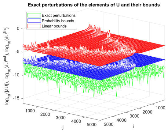
In Figure 1, we display the entries of the exact perturbation , together with the entries of the asymptotic and the probabilistic bound . The desired lower bound probability is set to , and the scaling factor for finding the probabilistic estimates is 1000. As a result, the actual probability is equal to , since all entries of exceed the corresponding entries of . As already mentioned, this phenomenon is due to the conservatism of the Markov inequality. The eigenvalue perturbations , together with their asymptotic estimate and probability estimate , are shown in Figure 2. There is no eigenvalue whose probability perturbation bound is smaller than the actual , which yields accuracy instead of the reference value of . Due to the equal spacing between the eigenvalues, the sensitivity of all invariant subspaces is the same in this case (Figure 3).
Figure 1.
The entries of the matrix and their asymptotic and probabilistic bounds for Example 4.
Figure 2.
The eigenvalue perturbations and their asymptotic and probabilistic bounds for Example 4.
Figure 3.
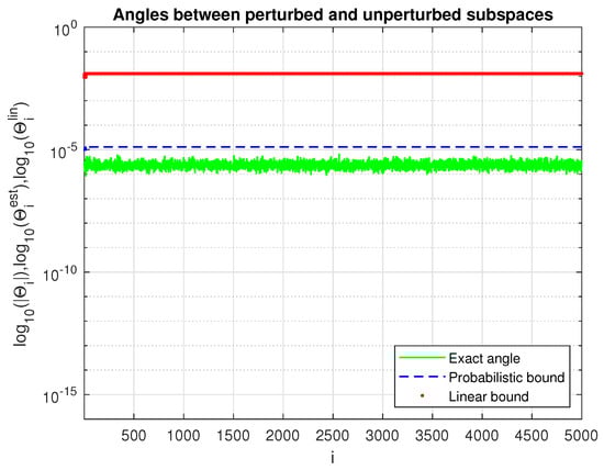
Angles between the perturbed and unperturbed invariant subspaces and their asymptotic and probabilistic bounds for Example 4.
Clearly, the probabilistic estimates are much closer to the actual perturbations than the linear deterministic bounds are.
Example 5.
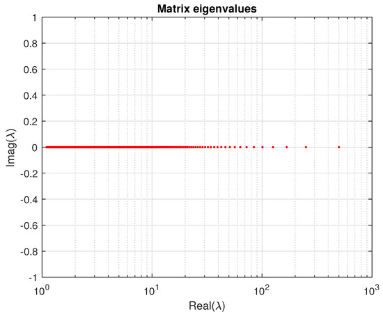
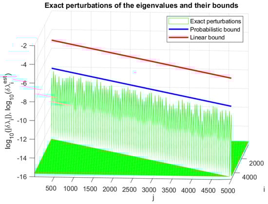
In this example, the eigenvalues of A are set to and are thus distributed between and 501. The norm of the matrix is equal to . The eigenvalues of A are shown in Figure 4.
Figure 4.
The matrix eigenvalues for Example 5.
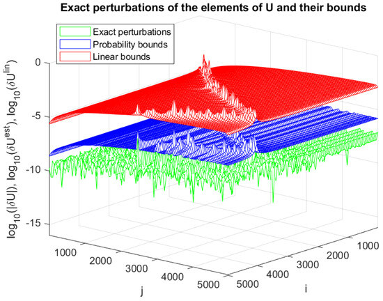
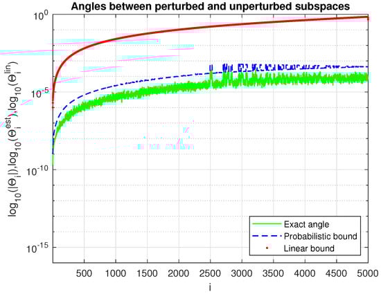
In Figure 5, Figure 6 and Figure 7, we present the matrix , the eigenvalue perturbations, and the angles between the perturbed and unperturbed invariant subspaces, respectively, as well as their asymptotic and probabilistic bounds for . Due to the decreasing separation between the eigenvalues, the sensitivity of the invariant subspace increases with the index i. As in the previous example, the actual probabilistic bounds for the eigenvector matrix and for the eigenvalues again reach .
Figure 5.
The entries of the matrix and their asymptotic and probabilistic bounds for Example 5.
Figure 6.
The eigenvalue perturbations and their asymptotic and probabilistic bounds for Example 5.
Figure 7.
Angles between the perturbed and unperturbed invariant subspaces and their asymptotic and probabilistic bounds for Example 5.
Note that in both examples, the linear estimates correctly reflect the changes in the corresponding exact quantities.
5. Conclusions
In this paper, we have presented strict asymptotic perturbation bounds for the eigenvalues, eigenvectors, and invariant subspaces of symmetric and Hermitian matrices. The use of the splitting operator method enables a unified treatment with the perturbation analysis of the Schur form [24] and the generalized Schur form [32]. Since the deterministic bounds derived may become conservative for high-order matrices, we have introduced probabilistic bounds based on the Markov inequality. These probabilistic bounds are easily obtained from the asymptotic bounds and allow a substantial reduction in the perturbation estimates with a guaranteed probability that is close to one in practice. As shown by the examples, an appealing aspect of the new bounds for symmetric matrices is that they can be determined with low requirements in terms of memory and volume of computational effort.
Author Contributions
Conceptualization, M.K. and P.H.P.; methodology, P.H.P.; software, P.H.P.; validation, M.K. All authors have read and agreed to the published version of the manuscript.
Funding
This research received no external funding.
Institutional Review Board Statement
Not applicable.
Informed Consent Statement
Not applicable.
Data Availability Statement
The datasets generated during the current study are available from the authors upon reasonable request.
Acknowledgments
The authors are grateful to the reviewers for their remarks and suggestions that helped to improve the manuscript.
Conflicts of Interest
The authors declare that the research was conducted in the absence of any commercial or financial relationship that could be construed as a potential conflict of interest.
Notation
| , | the set of complex numbers; |
| , | the space of complex matrices; |
| , | a matrix with entries ; |
| , | the jth column of A; |
| , | the ith row of an matrix A; |
| , | the jth column of an matrix A; |
| , | the strictly lower triangular part of A; |
| , | the matrix of absolute values of the elements of A; |
| , | the Hermitian transpose of A; |
| , | the zero matrix; |
| , | the identity matrix; |
| , | the perturbation of A; |
| , | the spectral norm of A; |
| , | the Frobenius norm of A; |
| , | equality by definition; |
| ⪯, | partial order: if , then means ; |
| , | the subspace spanned by the columns of X; |
| , | the orthogonal complement of U, ; |
References
- Kato, T. Perturbation Theory for Linear Operators, 2nd ed.; Springer: Berlin/Heidelberg, Germany, 1995; ISBN 978-0-540-58661-6. [Google Scholar]
- Wilkinson, J. The Algebraic Eigenvalue Problem; Clarendon Press: Oxford, UK, 1965; ISBN 978-0-19-853418-1. [Google Scholar]
- Parlett, B.N. The Symmetric Eigenvalue Problem; Society of Industrial and Applied Mathematics: Philadelphia, PA, USA, 1998. [Google Scholar] [CrossRef]
- Stewart, G.W.; Sun, J.-G. Matrix Perturbation Theory; Academic Press: New York, NY, USA, 1990; ISBN 978-0126702309. [Google Scholar]
- Bhatia, R. Perturbation Bounds for Matrix Eigenvalues; Society of Industrial and Applied Mathematics: Philadelphia, PA, USA, 2007; ISBN 978-0-898716-31-3. [Google Scholar] [CrossRef]
- Stewart, G. Matrix Algorithms; Vol. II: Eigensystems; SIAM: Philadelphia, PA, USA, 2001; ISBN 0-89871-503-2. [Google Scholar]
- Chatelin, F. Eigenvalues of Matrices; Society of Industrial and Applied Mathematics: Philadelphia, PA, USA, 2012; ISBN 978-1-611972-45-0. [Google Scholar] [CrossRef]
- Sun, J.-G. Stability and Accuracy. Perturbation Analysis of Algebraic Eigenproblems; Technical Report; Department of Computing Science, Umeå University: Umeå, Sweden, 1998; pp. 1–210. [Google Scholar]
- Li, R. Matrix perturbation theory. In Handbook of Linear Algebra, 2nd ed.; Hogben, L., Ed.; CRC Press: Boca Raton, FL, USA, 2014; pp. 21-1–21-20. [Google Scholar]
- Barlow, J.; Slapničar, I. Optimal perturbation bounds for the Hermitian eigenvalue problem. Linear Algebra Appl. 2000, 309, 19–43. [Google Scholar] [CrossRef][Green Version]
- Mathias, R. Quadratic residual bounds for the Hermitian eigenvalue problem. SIAM J. Matrix Anal. Appl. 1998, 19, 541–550. [Google Scholar] [CrossRef]
- Stewart, G.W. Error and perturbation bounds for subspaces associated with certain eigenvalue problems. SIAM Rev. 1973, 15, 727–764. [Google Scholar] [CrossRef]
- Sun, J.-G. Perturbation expansions for invariant subspaces. Linear Algebra Appl. 1991, 153, 85–97. [Google Scholar] [CrossRef][Green Version]
- Ipsen, I.C.F. An overview of relative sin(Θ) theorems for invariant subspaces of complex matrices. J. Comp. Appl. Math. 2000, 123, 131–153. [Google Scholar] [CrossRef]
- Veselić, K.; Slapničar, I. Floating-point perturbations of Hermitian matrices. Linear Algebra Appl. 1993, 195, 81–116. [Google Scholar] [CrossRef][Green Version]
- Greenbaum, A.; Li, R.-C.; Overton, M.L. First-order perturbation theory for eigenvalues and eigenvectors. SIAM Rev. 2020, 62, 463–482. [Google Scholar] [CrossRef]
- Barbarino, G.; Serra–Capizzano, S. Non-Hermitian perturbations of Hermitian matrix–sequences and applications to the spectral analysis of the numerical approximation of partial differential equations. Numer. Linear Algebra Appl. 2020, 27, 31. [Google Scholar] [CrossRef]
- Davis, C.; Kahan, W.M. The Rotation of Eigenvectors by a Perturbation. III. SIAM J. Numer. Anal. 1970, 7, 1–46. [Google Scholar] [CrossRef]
- Nakatsukasa, Y. Sharp error bounds for Ritz vectors and approximate singular vectors. Math. Comput. 2018, 89, 1843–1866. [Google Scholar] [CrossRef]
- Wang, W.-G.; Wei, Y. Mixed and componentwise condition numbers for matrix decompositions. Theor. Comput. Sci. 2017, 681, 199–216. [Google Scholar] [CrossRef]
- Carlsson, M. Spectral perturbation theory of Hermitian matrices. In Bridging Eigenvalue Theory and Practice—Applications in Modern Engineering; Carpentieri, B., Ed.; IntechOpen: London, UK, 2025; ISBN 978-1-83634-248-9. [Google Scholar] [CrossRef]
- Li, R.-C.; Nakatsukasa, Y.; Truhar, N.; Wang, W.-G. Perturbation of multiple eigenvalues of Hermitian matrices. Linear Algebra Appl. 2012, 437, 202–213. [Google Scholar] [CrossRef]
- Konstantinov, M.; Petkov, P. Perturbation Methods in Matrix Analysis and Control; NOVA Science Publishers, Inc.: New York, NY, USA, 2020; Available online: https://novapublishers.com/shop/perturbation-methods-in-matrix-analysis-and-control (accessed on 4 October 2025).
- Petkov, P. Componentwise perturbation analysis of the Schur decomposition of a matrix. SIAM J. Matrix Anal. Appl. 2021, 42, 108–133. [Google Scholar] [CrossRef]
- Golub, G.H.; Van Loan, C.F. Matrix Computations, 4th ed.; The Johns Hopkins University Press: Baltimore, MD, USA, 2013; ISBN 978-1-4214-0794-4. [Google Scholar]
- The MathWorks, Inc. MATLAB, Version 9.9.0.1538559 (R2020b); The MathWorks, Inc.: Natick, MA, USA, 2020. Available online: https://www.mathworks.com (accessed on 4 October 2025).
- Björck, A.; Golub, G. Numerical methods for computing angles between linear subspaces. Math. Comp. 1973, 27, 579–594. [Google Scholar] [CrossRef]
- Bai, Z.; Demmel, J.; Mckenney, A. On computing condition numbers for the nonsymmetric eigenproblem. ACM Trans. Math. Softw. 1993, 19, 202–223. [Google Scholar] [CrossRef]
- Petkov, P. Probabilistic perturbation bounds of matrix decompositions. Numer. Linear Algebra Appl. 2024, 31, 1–40. [Google Scholar] [CrossRef]
- Petkov, P. Probabilistic perturbation bounds for invariant, deflating and singular subspaces. Axioms 2024, 13, 597. [Google Scholar] [CrossRef]
- Papoulis, A. Probability, Random Variables and Stochastic Processes, 3rd ed.; McGraw Hill, Inc.: New York, NY, USA, 1991; ISBN 0-07-048477-5. [Google Scholar]
- Zhang, G.; Li, H.; Wei, Y. Componentwise perturbation analysis for the generalized Schur decomposition. Calcolo 2022, 59, 19. [Google Scholar] [CrossRef]


Disclaimer/Publisher’s Note: The statements, opinions and data contained in all publications are solely those of the individual author(s) and contributor(s) and not of MDPI and/or the editor(s). MDPI and/or the editor(s) disclaim responsibility for any injury to people or property resulting from any ideas, methods, instructions or products referred to in the content. |
© 2025 by the authors. Licensee MDPI, Basel, Switzerland. This article is an open access article distributed under the terms and conditions of the Creative Commons Attribution (CC BY) license (https://creativecommons.org/licenses/by/4.0/).