1. Introduction
The reduction in both the volume and radioactivity of high-level wastes prior to disposal, coupled with the recovery of unused uranium and plutonium, has been extensively researched. The initial breakthrough in solvent extraction for obtaining pure uranium and plutonium was achieved through the development of the PUREX process (Plutonium and Uranium Recovery by Extraction) [
1]. Tri-n-butyl phosphate (TBP) is a crucial extractant for uranium, plutonium, zirconium, and other metals in liquid–liquid extraction processes used in the atomic energy, hydrometallurgical, and chemical industries. In solvent extractions, TBP is combined with either a polar or nonpolar diluent. This combination modifies the density, facilitating phase separation, and reduces viscosity, thereby enhancing flow and kinetic properties [
1,
2,
3,
4,
5,
6,
7,
8]. Thus, TBP and its complexes with organic solutes are viscous and possess densities that are relatively close to that of the aqueous phase in typical liquid–liquid solvent extraction systems. In these systems, viscosity is a crucial transfer property, significantly impacting the scale-up of liquid applications [
9].
Due to its importance, researchers have made significant efforts to experimentally determine the viscosities of various TBP-diluent systems. In 2007, Tian et al. [
10] measured the densities and viscosities of the binary mixtures of TBP with hexane and dodecane systems. Following this work, in 2008, Fang et al. [
11] measured these experimental values using cyclohexane and n-heptane with the binary mixtures of TBP at atmospheric pressure in the whole composition range and over different temperatures. Fang reported that when the Grunberg Nissan equation was used to measure viscosity, the experimental data were measured with less than 1% average absolute deviation (ADD) at temperatures (from 288 to 308) K. Sagdeev et al. [
12] in 2013 measured the density and viscosity of n-heptane over a wider temperature range from 298 K to 470 K using the hydrostatic weighing and falling-body techniques. They calculated the ADD of 0.21% to 0.23% between the present and reported measurements of the density for n-heptane. In the same year, Basu et al. [
2] obtained the partial molar volumes of the respective components using a binary mixture of TBP with hexane, heptane, and cyclohexane at different temperatures from (298.15 to 323.15) K. Basu reported that a binary mixture of TBP with hexane could achieve a consistent negative deviation from ideality. Most recently, in 2018, Billah et al. [
3] measured densities, viscosities, and refractive indices for the binary mixtures of TBP under atmospheric pressure with toluene and ethylbenzene over the entire range of composition, and at different temperatures from T = (303.15 to 323.15) K.
Artificial Intelligence (AI) and machine learning (ML) have been extensively applied across all the areas of computational science, including biomedical sciences, drug delivery, chemistry, and material sciences, to predict the future behavior of systems based on historical data [
13,
14,
15,
16,
17,
18]. However, in the field of computational chemistry, conventional methods for measuring the viscosity of TBP mixture systems have primarily focused on pure liquids and binary mixtures. Therefore, predictive models for the viscosity of TBP mixtures are needed for practical process calculations and equipment design. Despite their widespread use, these traditional methods are time-consuming, tedious, and require a multistage preparation process, which can be harmful to human health and the environment due to the use of toxic organic solvents. Consequently, machine learning-based models that provide reliable viscosity predictions for liquids are crucial.
The literature survey revealed that, to date, no studies have modeled the viscosity of TBP mixtures using ML techniques. This research gap inspired us to propose ML models to accurately predict the viscosity of TBP diluted in solvents using experimental data obtained from the literature [
2,
3,
10,
11]. In this study, for the first time, we propose an accurate and efficient artificial neural network (NN) to predict the relative viscosity of TBP. Additionally, we demonstrate that ML models can predict the viscosity of TBP mixtures with a high degree of accuracy. Among the five ML models developed in this study, the NN model emerges as a suitable option for accurately predicting the viscosity of TBP mixtures with a lower margin of deviation (MOD) compared to the other regular ML models.
The novelty of this research lies in its comprehensive comparison of different ML models to predict TBP mixture viscosities, which could significantly streamline industrial processes and reduce exposure to toxic solvents. The second section provides a comprehensive overview of the experimental database, feature visualization, machine learning model setup, and statistical analysis.
Section 3 explores our findings, emphasizing the advantages of employing various machine learning techniques and showcasing the impressive effectiveness of each model.
Section 4 comprises the discussion, and finally,
Section 5 summarizes our findings, underscoring the model’s potential in enhancing viscosity refinement and advancing our knowledge of TBP fluid properties.
2. Materials and Methods
The proposed algorithm to predict the dynamic viscosity of TBP mixtures is illustrated in
Figure 1. The dataset comprises 511 measurements for TBP mixtures with temperature-based density across different compositions. We pre-processed the data by standardizing it to ensure uniform scaling across all the features, and we reduced the dimensionality of the data to facilitate efficient training.
To ensure a fair comparison, we utilized five different ML algorithms—Logistic Regression (LR), Support Vector Regression (SVR), random forest (RF), Extreme Gradient Boosting (XGBoost), and neural network (NN)—employing identical experimental data points (4599 = 511 measurements × 9 features per measurement) for the viscosity of TBP mixtures across various compositions, densities, and temperatures. We hypothesized that the ML models can accurately predict viscosities compared to the actual (observed) values. To evaluate this hypothesis, we conducted a two-sample
t-test on the predicted viscosity values. Further details regarding the block diagram in
Figure 1 will be elaborated in the subsequent sections.
2.1. Experimental Database and Feature Visualization
The databases for this study were compiled from data reported in the literature. A total of 511 experimental points for TBP mixtures with temperature-based density, encompassing various compositions and including hexane, dodecane, cyclohexane, n-heptane, toluene, and ethylbenzene, were gathered from multiple scientific publications [
3,
10,
11]. In the original dataset, there are nine descriptors (features), including temperature, density, and seven compositions, used to estimate viscosity.
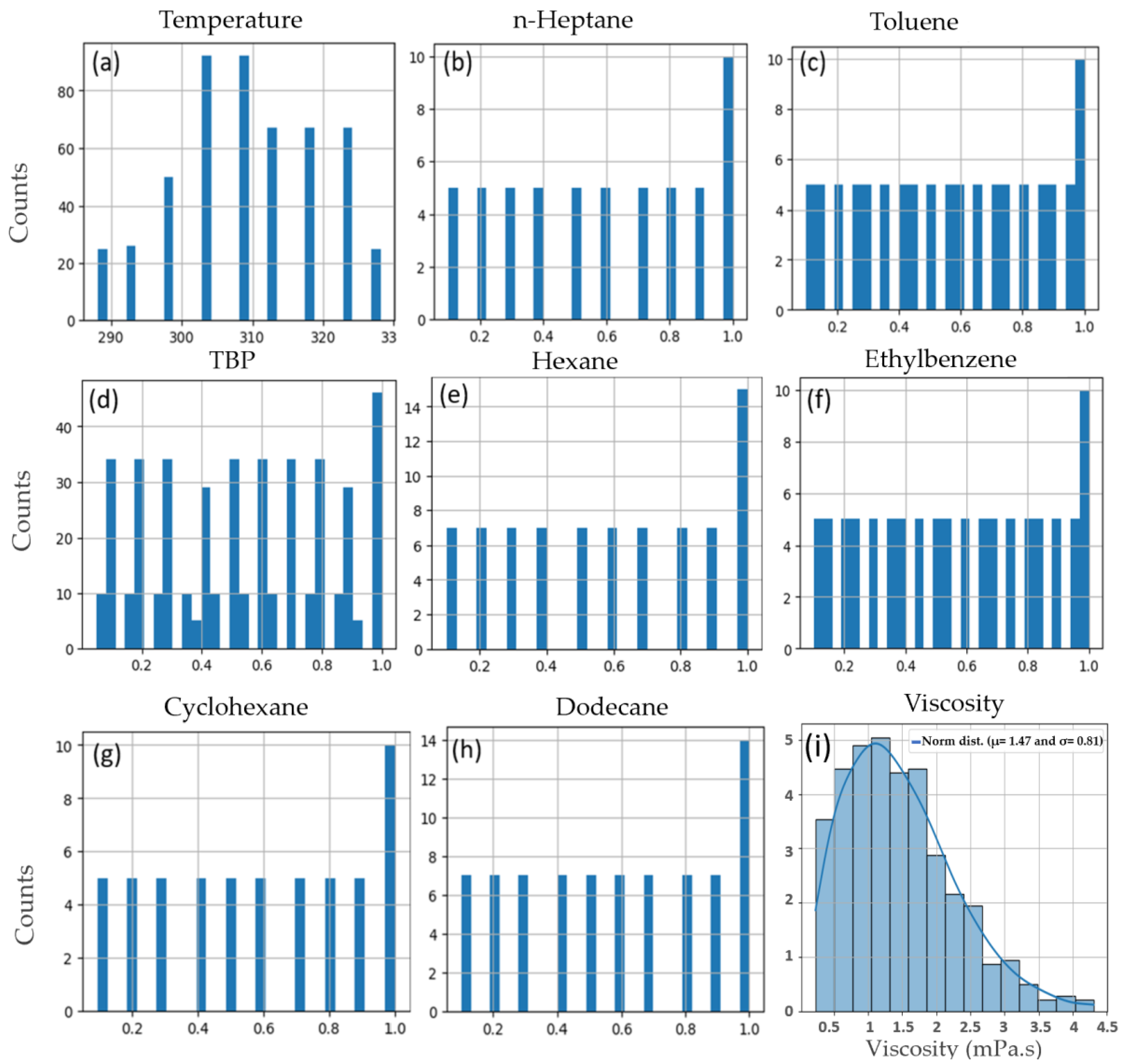
Figure 2a–h depict the distribution of the values in the dataset, with the x-axis representing the values and the y-axis indicating the frequency of each value.
Figure 2i illustrates the viscosity changes in the dataset, showing a normal distribution with parameters N (1.47, 0.81).
2.2. Correlation Matrix
To assess the relationships between the features and the target variable (viscosity), the Pearson product–moment correlation coefficient was utilized [
19]. The correlation heatmap in
Figure 3 reveals significant insights into the relationships between the various factors influencing the viscosity of TBP mixtures. Temperature shows a moderate negative correlation with viscosity (−0.36), indicating that higher temperatures lead to lower viscosities. TBP composition has a strong positive correlation with viscosity (0.86) and density (0.80), suggesting that higher TBP content increases both viscosity and density. In contrast, hexane composition demonstrates a moderate negative correlation with viscosity (−0.38) and density (−0.55), implying that more hexane results in lower viscosity and density. Other components like cyclohexane, n-heptane, dodecane, and toluene show weaker correlations with viscosity, highlighting that their impacts are less significant compared to TBP and hexane. These correlations underscore the dominant influence of TBP and hexane compositions on the viscosity and density of the mixtures, while temperature also plays a crucial role in modifying these properties.
The exploration of the relationship between viscosity, temperature, and TBP composition is crucial because viscosity significantly affects the efficiency of industrial processes involving TBP. Temperature variations impact viscosity, thereby influencing mixing and separation processes. TBP is a primary component in these mixtures, and its concentration directly affects the physical properties of the mixture. Understanding these relationships allows us to develop accurate predictive models, enhancing process control, efficiency, and safety in industrial applications.
Figure 4 illustrates the relationships between viscosity, temperature, and TBP composition.
Figure 4a depicts the association between temperature (K) and viscosity (mPa·s). The scatter plot, supplemented with a regression line, shows a negative correlation, indicating that viscosity decreases as temperature increases. The distribution plots at the top and right side of the scatter plot further emphasize this trend, revealing a broad spread of viscosity values at lower temperatures and a tighter distribution at higher temperatures.
Figure 4b presents a 3D surface plot of viscosity as a function of temperature (K) and TBP composition. This visualization shows that viscosity decreases not only with increasing temperature but also as TBP composition increases. The gradient in the color scale, from red (higher viscosity) to blue (lower viscosity), further confirms that higher temperatures and TBP compositions contribute to lower viscosity values. This indicates that both higher temperature and higher TBP concentration synergistically reduce the viscosity of the mixture.
2.3. Feature Selection and Principal Component Analysis
Principal Component Analysis (PCA) was utilized to reduce data dimensionality [
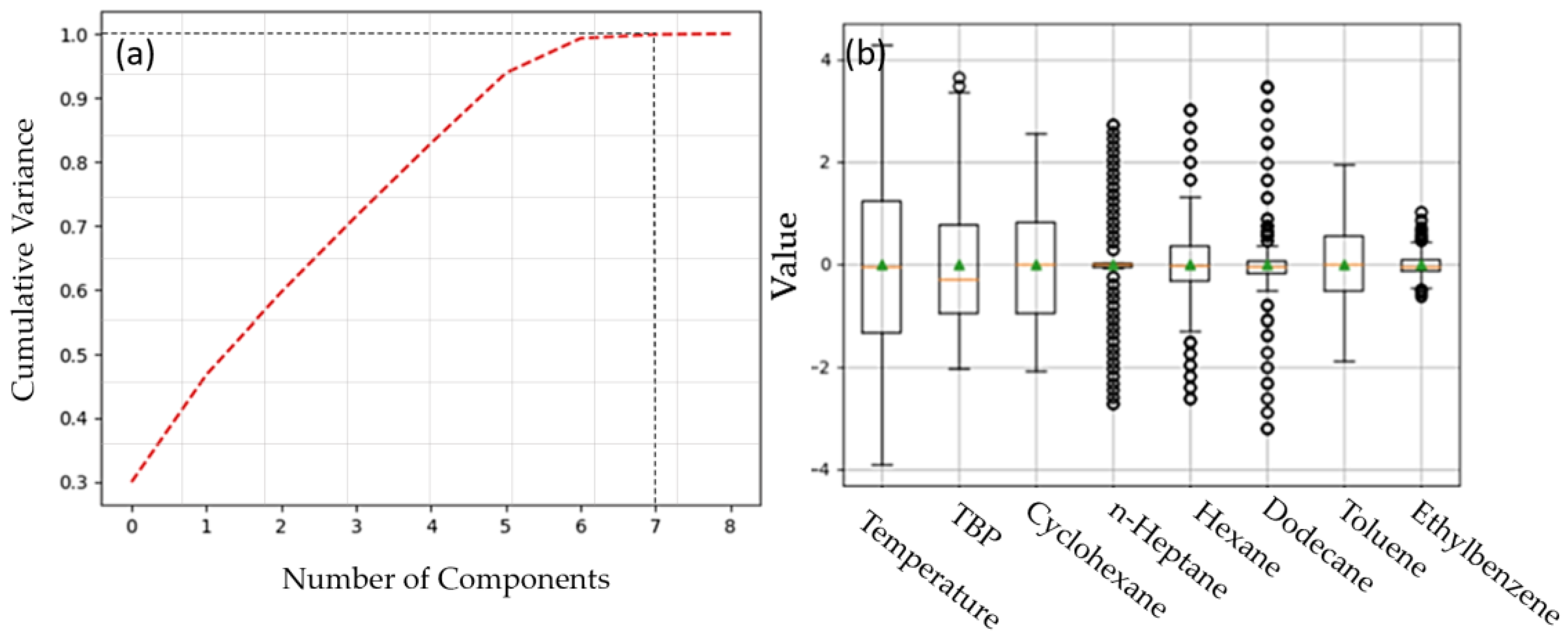
20]. In achieving this, PCA effectively transforms data points from a high-dimensional to a low-dimensional space, preserving essential linear structures throughout the process. The robust optimality of the resultant low-dimensional embedding stems from the precise mathematical foundation underlying PCA. For feature selection, we employed pairwise correlation analysis in Python, setting Pearson correlation coefficients between 5% and 95% to identify highly correlated features. Subsequently, we applied PCA to these correlated features, reducing dimensionality to eight principal components, effectively capturing over 99% of the variability within the dataset.
Figure 5a illustrates the explained variance for all the features, while
Figure 5b depicts the variation distribution of the selected significant features, excluding density in the training of the ML algorithms. This analysis reveals that temperature exhibits the highest variation, whereas n-heptane composition shows the lowest variation among the features considered.
To elaborate further, the input variables considered were temperature and the compositions (
Xi) of solvents for each species. The viscosity functionality of the solvents is outlined below:
where
X1 to
X7 are the solvents and
T = (288.15, 293.15, 298.15, 303.15, 308.15, 313.15, 318.15, 323.15, and 328.15)
K are the experimental temperatures used to measure the compositions. After identifying and collecting the data set, the next step was to select the ML models to predict the viscosity. To do so, for comparison purposes, we trained five different ML algorithms including SVR, RF, LR, XGB, and NN, which will be explained in the following section. To train these models, we randomly split our dataset to 80% for training and 20% for validation and testing. In this study, the training set was used to generate the ML model, and the test set was utilized to investigate the prediction capability and to validate the trained model.
2.4. Machine Learning Models
All the models discussed in this section were built in Python 3.8 with Scikit-Learn 1.1.3, Keras 2.9, TensorFlow 2.9.1 libraries trained by an RTX 3090 GPU with 24 GB memory, and CUDA 11.4.
2.4.1. Support Vector Regression (SVR)
The SVR algorithm approach’s function approximation is an optimization problem, aiming to minimize the gap between predicted and desired outputs [
21,
22,
23]. Given that our problem lacked linear separability in the input space, we employed a kernel to map the data to a higher-dimensional space, known as kernel space, where linear separability could be achieved. In this investigation, we utilized the Scikit-learn framework [
24] (version 1.1.3) library with SVR class with parameters including a radial basis function (‘RBF) kernel with a 0.001 tolerance for stopping criterion, and the regularization parameter
C = 1 have been used. We performed a linear SVR which is expressed below:
where
X,
ω = (
ω1,
ω2, …,
ωn) ∈
Rn,
b ∈
R, and
T are, respectively, the input or support vectors, the weight vector, the intercept, and transpose operator. The optimization problem for training the linear SVR is given by the following:
where
C is a positive regularization parameter (
C = 1), the penalty for incorrectly estimating the output associated with input vectors.
2.4.2. Gradient Boosted Decision Trees (XGBoost)
The XGBoost regressor employed a combination of 100 decision trees to mitigate the risk of overfitting encountered by each individual tree. XGBoost utilized a boosting technique, sequentially combining weak learners, such that each subsequent tree rectified the errors of its predecessor [
25,
26]. In this work, the XGBoost model was developed with a learning rate of 0.3 and the number of estimators = 100.
2.4.3. Random Forest (RF)
By utilizing different subsets of the available features, numerous independent decision trees can be simultaneously constructed on various sections of the training data. Bootstrapping ensures that each decision tree within the random forest is unique, contributing to the reduction in RF variance [
27]. We found 100 trees in the forest to be optimum in our RF model.
2.4.4. Logistic Regression (LR)
The main advantage of LR is to avoid confounding effects by analyzing the association of all the variables together [
28,
29]. In this work, we used the “L2” regularization method which is a ridge regression and can add a squared magnitude of coefficients as the penalty term to the loss function regularization.
2.4.5. Neural Network Architecture
In the NN architecture, we implemented a feed-forward backpropagation approach to adjust the weights and determine the optimal mapping between the input features and the target output [
30,
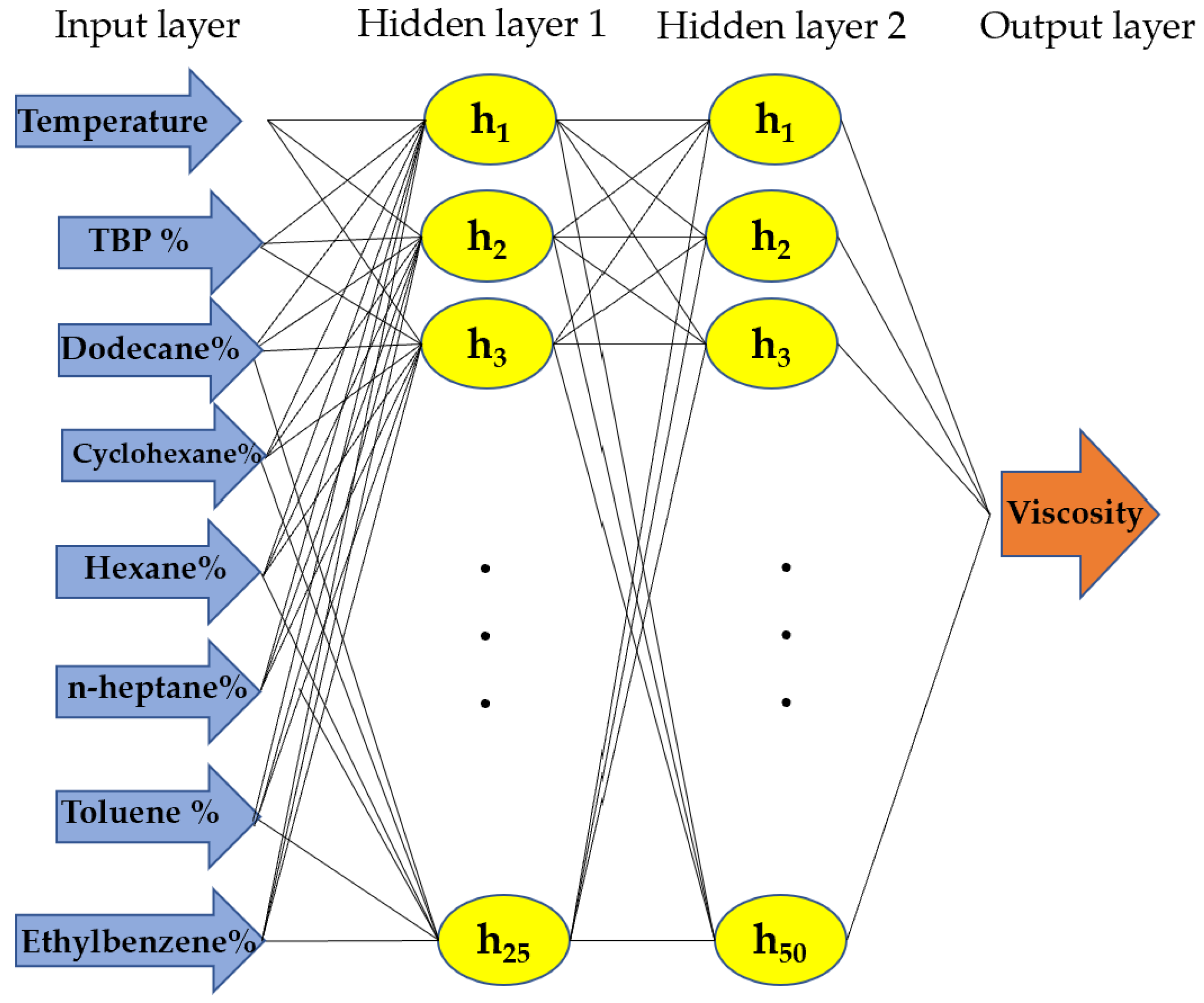
31]. The architecture of the feedforward network utilized in this study is depicted in
Figure 6, comprising two hidden layers with 25 and 50 neurons for the first and second hidden layers, respectively. The ‘ReLU’ activation function was employed to propagate only positive weights, as specified in Equation (4). To select the optimal parameters, we employed a cross-validated approach using the GridSearchCV method with 5-fold cross-validation in Python [
32,
33].
2.5. Performance Metrics
The trained models’ performance was evaluated using three parameters: Mean Absolute Error (
MAE), Mean Squared Error (
MSE), and the adjusted correlation coefficient (
R2). Regression analysis was employed to evaluate the network’s capability for ternary viscosity prediction, with the coefficient of determination serving as a metric to gauge the correlation between the trained model and the experimental data. The performance metrics used in this study were defined as below:
where
N is the number of viscosity data points,
is the ith observed value of the viscosity,
is the predicted viscosity with the ML model,
is the average value of the experimental viscosity data, and
p is the number of predictors.
2.6. Statistical Analysis
In RStudio Version 2022.07.0 + 548, statistical analysis was conducted to ascertain if there were any statistically significant differences between the observed and predicted viscosity values for each ML model. It was assumed that the feature distribution was normal, and the samples were drawn from independent features. Subsequently, for each model, the null hypothesis was assessed by computing the mean (
µ) for the viscosity values to test whether
µobserved =
µpredicted. The margin of deviation (
MOD) was used to calculate the error bars as defined below:
3. Results
In this section, we discuss the performance of the various approaches and the optimal parameters for the developed ML algorithms. The developed models were trained on 408 observations with eight features (totaling 3264 data points) and tested on 103 observations with eight features (totaling 824 data points) across temperatures ranging from 288.15 K to 328.15 K.
The learning curves for the NN model are depicted in
Figure 7, illustrating that the NN model began to converge after 20 epochs.
Table 1 presents a comparison of all the developed models’ performance in terms of adjusted
R2,
MSE, and
MAE. As indicated in
Table 1, the NN model achieved the highest performance with an MSE of 0.157% and an adjusted
R2 of 99.97%. Following the NN model, in descending order of performance, XGBoost, RF, SVR, and Logistic Regression attained adjusted
R2 values of 99.54%, 99.22%, 99.06%, and 93.10%, respectively, on the test dataset.
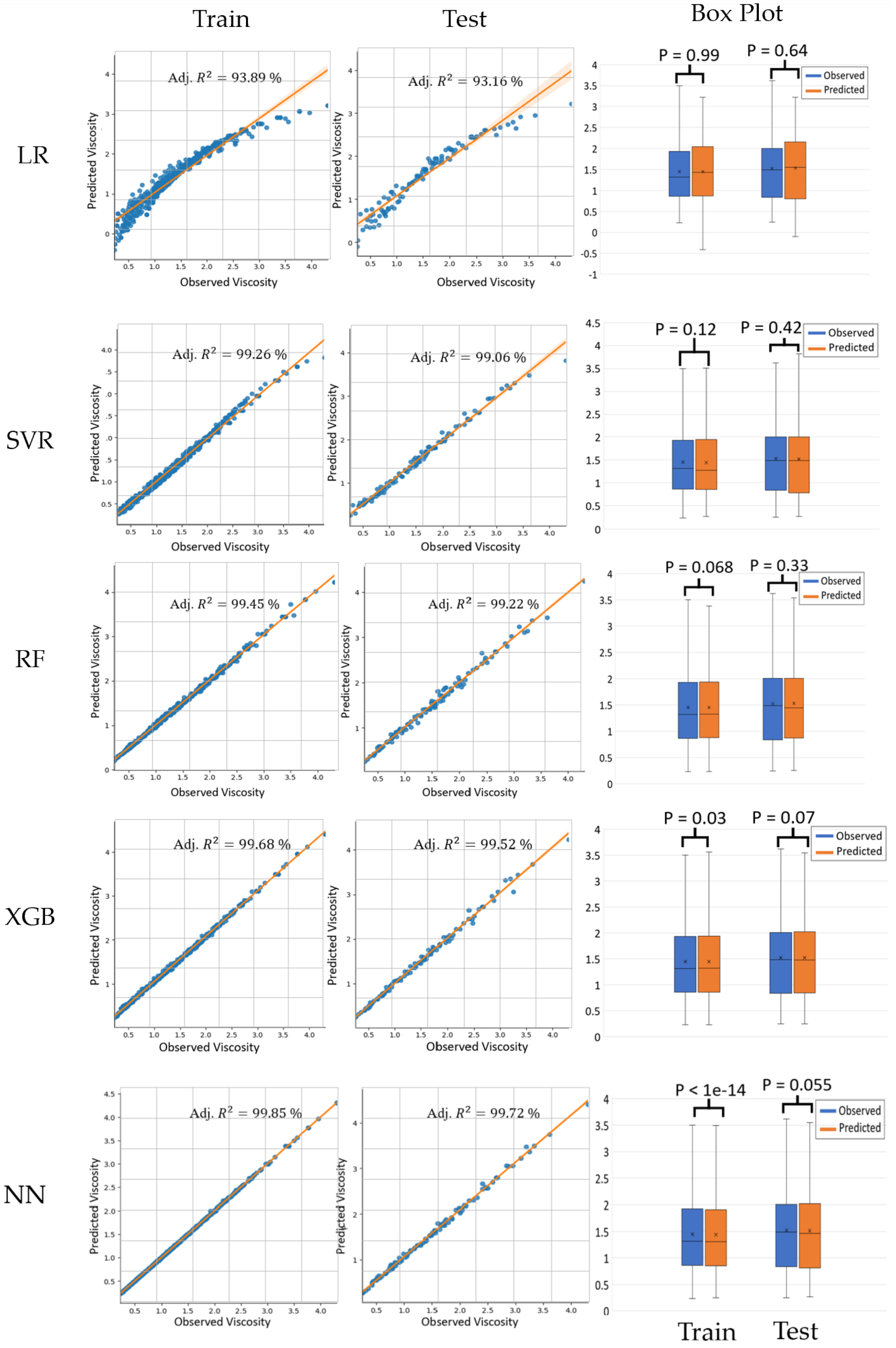
Figure 8 presents a comparative analysis of the five ML models—LR, SVR, RF, XGB, and NN—in predicting viscosity. The scatter plots for both the training and testing datasets illustrate the relationship between the observed and predicted viscosity, with the adjusted R-squared values indicating the model’s performance. LR exhibits the adjusted R-squared values of 93.89% and 93.16% for training and testing, respectively. SVR shows significantly higher values of 99.26% and 99.06%, while RF and XGB demonstrate even stronger performance with values exceeding 99.2% for both the datasets. NN outperformed all the trained models with the R-squared values of 99.85% and 99.72%. for training and testing, respectively. The accompanying box plots, with the
p-values from
t-tests, indicate that there are no statistically significant differences between the observed and predicted viscosities across all the models, except for NN (
p < 1 × 10
−14) and a marginal significance in the training set of XGB (
p = 0.03). This comprehensive evaluation highlights the superior predictive accuracy of NN and XGB models compared to LR, SVR, and RF for viscosity prediction.
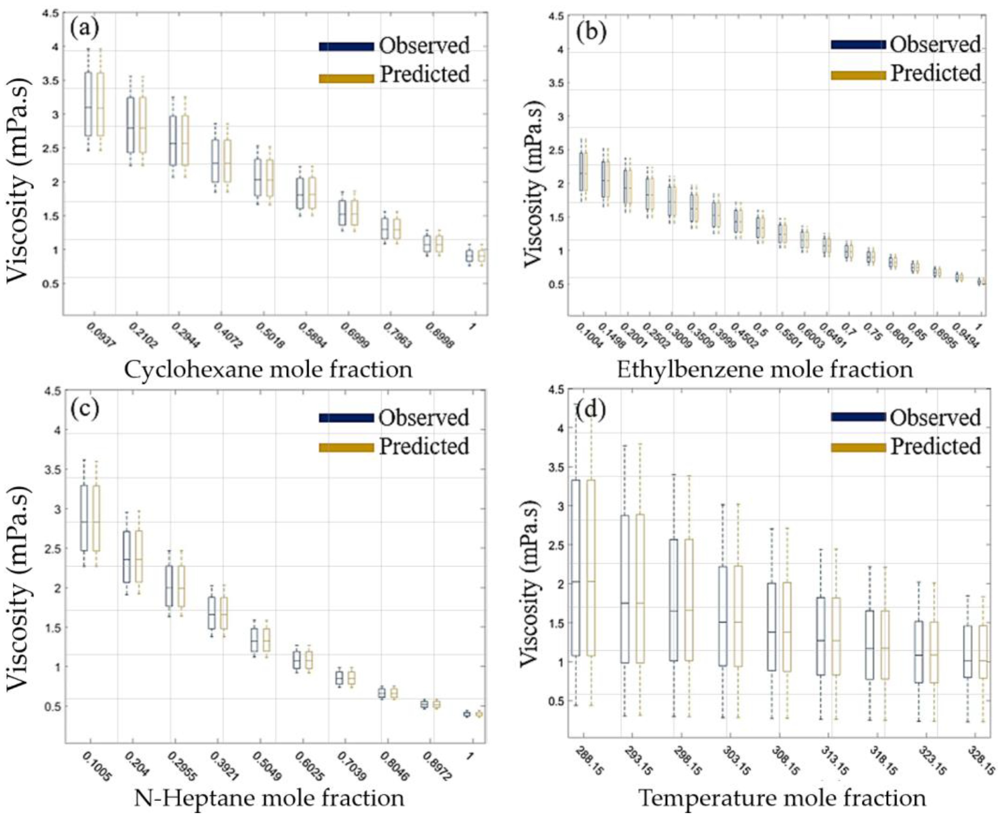
Figure 9 presents a comparative analysis of the observed and predicted viscosity values under varying conditions, depicted in four subplots.
Figure 9a illustrates the relationship between the viscosity and cyclohexane mole fraction, showing a decreasing trend as the mole fraction increases, with the predicted values closely aligning with the observed data.
Figure 9b examines the effect of the ethylbenzene mole fraction on viscosity, also demonstrating a decrease in the viscosity with increasing mole fraction, where the predicted values consistently match the observed values.
Figure 9c explores the viscosity variation with n-heptane mole fraction, revealing a similar decreasing trend, and the predicted values once again closely follow the observed data. Lastly,
Figure 9d shows the viscosity dependence on temperature, with the viscosity decreasing as the temperature rises, and the predicted values aligning well with the observed ones across different temperature points. Overall, the predictive model demonstrates a high degree of accuracy in estimating viscosity across different mole fractions and temperature conditions, as evidenced by the close match between the observed and predicted data.
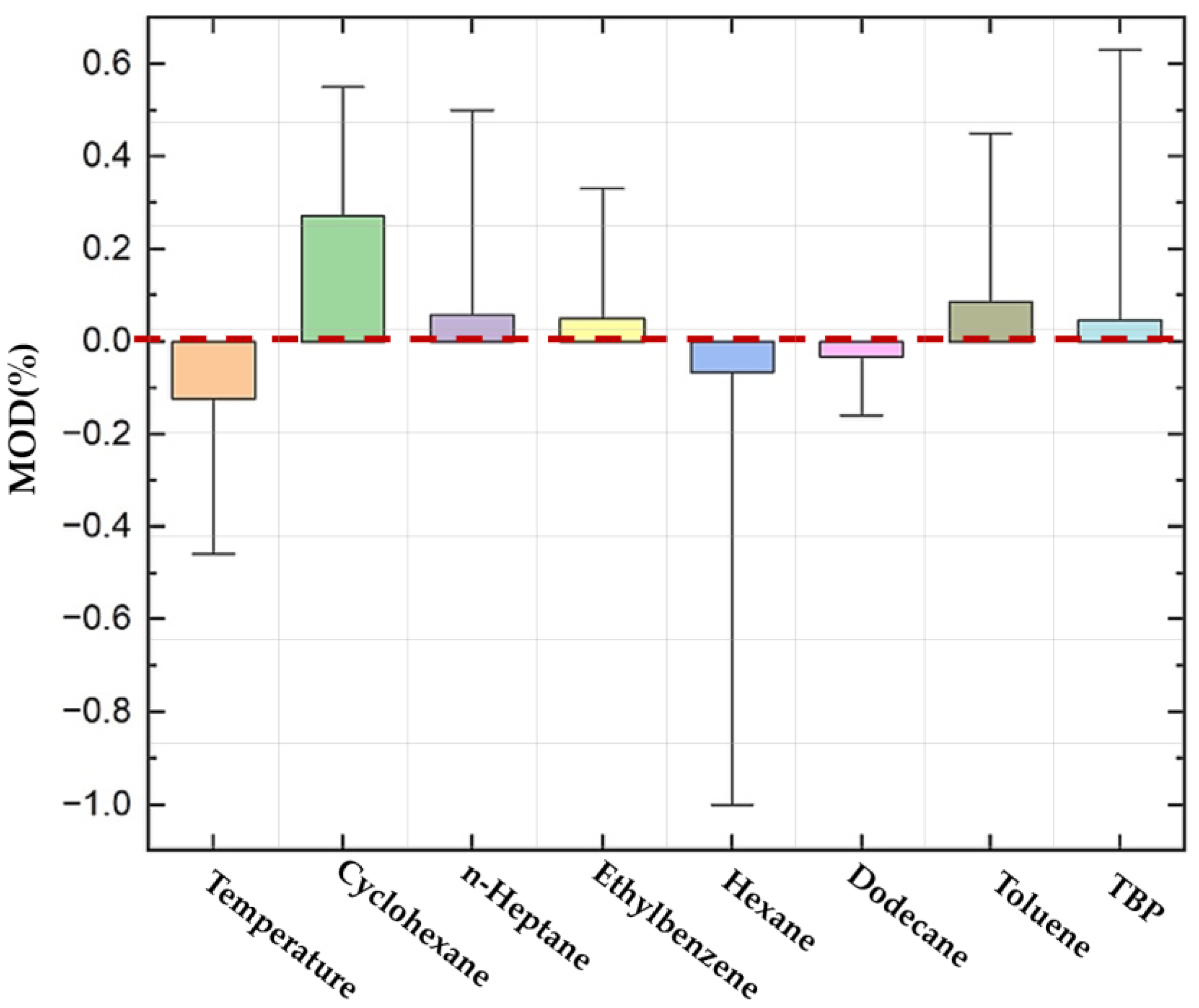
Figure 10 displays the
MOD percentages for viscosity predictions across various factors. Temperature has a median
MOD of approximately −0.1% (IQR: −0.35% to 0.15%), while cyclohexane shows a median
MOD of 0.2% (IQR: 0.05% to 0.45%). For n-heptane, the median
MOD is around 0.05% (IQR: −0.1% to 0.15%), and ethylbenzene shows a median
MOD of 0.05% (IQR: −0.05% to 0.15%). Hexane exhibits a median
MOD of 0.0% (IQR: −0.15% to 0.15%), dodecane a median MOD of 0.0% (IQR: −0.05% to 0.2%), toluene a median
MOD of 0.05% (IQR: −0.1% to 0.25%), and TBP a median
MOD of 0.0% (IQR: −0.05% to 0.2%). The results indicate good predictive accuracy, with most deviations being minor, and variability is lowest for ethylbenzene and TBP and highest for hexane and cyclohexane, demonstrating the model’s robust reliability across different chemical conditions and temperatures.
The computational cost analysis (
Table 2) reveals that the NN has the highest training time (6.5780 s) but a low inference time (0.0055 s), making it efficient for real-time predictions. XGBoost is the most efficient overall, with the lowest training (0.0029 s) and inference (0.0018 s) times. RF shows moderate costs, while SVR is extremely fast in both training (0.0010 s) and inference (0.0004 s). LR also has low computational costs, making it suitable for quick predictions. These results highlight the trade-offs between accuracy and computational efficiency for each model.
4. Discussion
This study aimed to predict the viscosity of TBP mixtures using five different machine learning models. The analysis included 408 observations with eight features (TBP, hexane, dodecane, cyclohexane, n-heptane, toluene, ethylbenzene, and temperature). The viscosity predictions spanned temperatures from 288.15 K to 328.15 K. The performance of each model was evaluated using metrics such as Mean Squared Error (MSE), Mean Absolute Error (MAE), and adjusted R2. The NN model outperformed the others with an MSE of 0.157% and an adjusted R2 of 99.97% on the test dataset; however, it needs a longer time for training with respect to other models. XGBoost, RF, and SVR followed with the adjusted R2 values of 99.54%, 99.22%, and 99.06%, respectively, while LR had the lowest performance with an adjusted R2 of 93.16%.
The NN model’s architecture, consisting of 25 neurons in the first hidden layer and 50 neurons in the second hidden layer, demonstrated superior predictive accuracy, particularly for the TBP + Ethylbenzene system, achieving a MOD of 0.049%. This highlights the NN model’s robustness and reliability in handling the non-linear relationships in the data. The MOD was analyzed across different solvents to assess the prediction accuracy further. Temperature showed a median MOD of approximately −0.1% with low variability, indicating consistent performance across different temperature ranges. Among the solvents, cyclohexane had the highest variability in MOD, while ethylbenzene and TBP exhibited the lowest, signifying stable predictions for these solvents. The findings from this study underscore the efficacy of the ML models in predicting the viscosity of complex mixtures like TBP. The high adjusted R2 values and low MSE indicate that these models can capture the intricate dependencies between the features, providing accurate viscosity predictions. This is particularly valuable for applications in chemical engineering where precise viscosity measurements are crucial.
A primary limitation of this study is the relatively small dataset size. Despite using techniques such as GridSearchCV for hyperparameter tuning and dropout methods to prevent overfitting, a larger dataset would likely improve model accuracy and generalizability. Moreover, the results of PCA suggest only reducing the dimension by one, which is not a significant reduction. Due to the small dataset size, we chose to retain all the compositional variables to ensure the models have sufficient information to make precise predictions. Reducing dimensions further using PCA could lead to the loss of important compositional information, which is vital for capturing the intricate relationships between viscosity and the components of the mixture. Then, we chose not to reduce more dimensions, as all the molecular compositions need to be considered to maintain the integrity and accuracy of our predictions. Future research should focus on expanding the dataset to include more compositions and temperature ranges, which would enhance the models’ robustness. Moreover, while this study focused on viscosity, incorporating additional physical properties such as density could provide a more comprehensive understanding of TBP mixtures. Exploring multi-output models that predict both viscosity and density simultaneously could be a promising direction for future work. Future works should also focus on assessing model performance by comparing the simulated and observed data using a more balanced metric like the Kling–Gupta efficiency [
34].
The successful application of the ML models in this study demonstrates their potential in computational chemistry, particularly in predicting the properties of complex mixtures. This approach can be extended to other chemical systems, facilitating more efficient and accurate property predictions. The integration of ML techniques in chemical engineering workflows could lead to significant advancements in process optimization, materials design, and quality control.
5. Conclusions
In this paper, we presented a comparative study of various machine learning (ML) models for predicting the viscosity of Tri-n-butyl phosphate (TBP) mixtures. The models evaluated included Logistic Regression (LR), Support Vector Regression (SVR), random forest (RF), Extreme Gradient Boosting (XGBoost), and neural network (NN). We utilized an extensive experimental dataset to train and test these models, employing Principal Component Analysis (PCA) for feature selection and dimensionality reduction.
Our primary hypothesis was that the ML models could accurately predict the viscosity of TBP mixtures, potentially outperforming the traditional experimental methods in terms of efficiency and safety. Based on our findings, this hypothesis was validated, particularly with the NN model, which achieved the highest accuracy with an MSE of 0.157% and an adjusted R2 of 99.72%. This model’s performance supports the feasibility of using ML to predict viscosity, thereby reducing the reliance on labor-intensive and hazardous traditional methods.
The investigated ML models demonstrated superior accuracy in predicting TBP viscosity, making it a reliable tool for industrial applications. Also, the ML models, once trained, can provide rapid predictions, significantly reducing the time required compared to traditional experimental methods, and reducing the need for direct handling of toxic solvents, thereby enhancing laboratory safety. The methodology can be extended to other chemical systems and different types of mixtures, showcasing its versatility. On the other hand, ML models are computationally intensive, requiring significant resources for training. The accuracy of the ML models is contingent on the quality and range of the training data, which in this study was limited to specific temperature ranges and compositions.
Future research should focus on expanding the experimental dataset to include a broader range of compositions and temperatures, enhancing the model’s robustness and accuracy. Additionally, incorporating more advanced ML techniques and exploring ensemble methods could further improve predictive performance. Predicting other related properties, such as density alongside viscosity, could provide a more comprehensive understanding of TBP mixtures. Addressing these areas will mitigate the current methodology’s disadvantages and open new avenues for applying ML in chemical process optimization.

