Diatomic: An Open-Source Excel Application to Calculate Thermodynamic Properties for Diatomic Molecules

Abstract

In this paper, I present Diatomic, an open-source Excel application that calculates molar thermodynamic properties for diatomic ideal gases. This application is very easy to use and requires only a limited number of molecular constants, which are freely available online. Despite its simplicity, Diatomic provides methodologies and results that are usually unavailable in general quantum chemistry packages. This application uses the general formalism of statistical mechanics, enabling two models to describe the rotational structure and two models to describe the vibrational structure. In this work, Diatomic was used to calculate standard molar thermodynamic properties for a set of fifteen diatomic ideal gases. A special emphasis was placed on the analysis of four properties (standard molar enthalpy of formation, molar heat capacity at constant pressure, average molar thermal enthalpy, and standard molar entropy), which were compared with experimental values. A molecular interpretation for the molar heat capacity at constant pressure, as an interesting pedagogical application of Diatomic, was also explored in this paper.

1. Introduction

Diatomic molecules are important in many areas of modern science, such as atmospheric chemistry [1,2], astrobiology [3], and ultracold physics [4]. Despite their simplicity, diatomic molecules are valuable models for understanding the relationship between structure and thermodynamic properties in more complex systems. For this purpose, the development of high-quality theoretical methods to calculate these properties is of paramount importance. Two main strategies have usually been adopted to improve the accuracy of these methods: (i) improving the description of the electronic structure [5,6,7,8], and (ii) implementing better models to describe the (rotational and vibrational) nuclear motions [9,10,11,12,13,14,15,16,17,18,19,20,21,22,23,24,25,26,27,28].

Obtaining more reliable information about the electronic structure has been achieved by (i) a high-level quantum method [5,6,7], (ii) a robust basis set [5,6,7], (iii) the extrapolation to the complete basis set (CBS) limit [5,6,7], (iv) the inclusion of relativistic and spin–orbit effects [5,6,7,8], and (v) a very good description of the electronic correlation [5,6,7].

The rotational structure is usually described by a classical approach since the temperatures of interest are normally much higher than the characteristic rotational temperatures. However, at low temperatures, it is important to adopt a quantum description of this structure to obtain accurate values [9].

At low and moderate temperatures, the vibrational structure can be reasonably described by the harmonic oscillator model [10]. However, this approach is known to overestimate the vibrational frequencies [10], leading to significant errors at high temperatures. To overcome this limitation, several correction methods have been applied [11,12,13,14,15,16,17,18,19,20,21,22,23,24,25,26,27,28]. Most of them can be classified into two groups: (i) methods that use empirical scaling factors to correct the harmonic frequencies [13,14,15,16,17,18], and (ii) methods that use anharmonic potentials [19,20,21,22,23,24,25,26,27,28].

The thermodynamic properties of a molecular system can be calculated using general quantum chemistry packages [29,30,31,32,33,34]. However, the required computational resources and level of expertise are considerable. The main difficulty in performing these calculations is probably the installation of such types of packages, which constitutes a very hard task for nonspecialized researchers or students.

In this work, I have developed an open-source Excel application to calculate thermodynamic properties for diatomic ideal gases. This application, called Diatomic, is very easy to use and requires only some basic knowledge of theoretical chemistry. In fact, a user of Diatomic only has to input a limited number of molecular constants (namely, the electronic ground state energy and the corresponding spin multiplicity, the atomic masses, the rotational symmetry number, the equilibrium bond length, the harmonic vibrational wave number, and the well depth of the Morse potential) to perform a calculation of this type. This information is freely available from online resources [35]. Additionally, the pressure and a set of fourteen temperatures must also be inputted.

Diatomic provides many features, often not available in general quantum chemistry packages, to perform and interpret this type of calculation. These include (i) two models (classical and quantum) describing the rotational structure, (ii) two models (harmonic and Morse) describing the vibrational structure, (iii) energies and Boltzmann populations for the quantum rotational model, (iv) energies and Boltzmann populations for both vibrational models implemented in the application, (v) molar thermodynamic properties as a function of temperature available in very easy to interpret and process tables, and (vi) availability of these tables organized by different criteria.

A future user of Diatomic should be interested in diatomic ideal gases for pedagogical and/or scientific purposes. I envision three main applications for this tool: (i) educational applications: professors and students can use this application to explore fundamental concepts in quantum chemistry and/or statistical mechanics without requiring special skills in computer science; (ii) research in experimental chemistry: researchers in this field can use Diatomic to easily predict the thermodynamic properties of diatomic ideal gases; and (iii) research in computational chemistry: researchers can explore specific features of Diatomic to rationalize the results of computational calculations.

Most of the aforementioned refinements to the electronic structure can be easily incorporated into Diatomic, as they solely impact the electronic energy. For this purpose, one only needs to search the literature for these corrected values. However, the goal of this work is not to obtain highly accurate values for the molar thermodynamic properties under study. Rather, I aim to demonstrate that users can achieve reliable results for these properties using Diatomic and freely available molecular data online. Additionally, since Diatomic is an open-source collaborative project, anyone can contribute by adding new vibrational potentials to the application.

Diatomic was used here to calculate these properties for fifteen ideal gases as a function of temperature and at a constant pressure. The chemical species studied correspond to all diatomic molecules that can be obtained by combining these five elements: H, N, O, F, and Cl.

These molecules are classified according to their symmetry (homonuclear or heteronuclear) and spin multiplicity (singlet, doublet, or triplet) (see

Table 1. Classification of the diatomic molecules under study.

Type	Number of Molecules	Molecules
Singlet homonuclear	4	H2, N2, F2, Cl2
Triplet homonuclear	1	O2
Singlet heteronuclear	3	HF, HCl, ClF
Doublet heteronuclear	4	OH, NO, OF, ClO
Triplet heteronuclear	3	NH, NF, NCl

).

2. Methods

2.1. General Formalism

According to the well-established formalism of statistical mechanics [36,37,38], all the most relevant thermodynamic properties of an ideal gas can be calculated from its partition function. For a molar canonical ensemble, which is equivalent to an isothermal-isobaric ensemble for an ideal gas, and within the Born–Oppenheimer approach, this partition function (Q(N_A, V, T)) can be calculated from its molecular components:

$$Q(N_A,V,T)={\displaystyle \frac{Z^{N_A}}{N_A!}}={\left(Z_{el}\right)}^{N_A}\times {\displaystyle \frac{{\left(Z_{transl}\right)}^{N_A}}{N_A!}}\times {\left(Z_{rot}\right)}^{N_A}\times {\left(Z_{vib}\right)}^{N_A}$$

(1)

In Equation (1), N_A is the Avogadro number and Z is the molecular partition function. In the same Equation, Z_el, Z_transl, Z_rot, and Z_vib are the (electronic, translational, rotational and vibrational) components of the partition function. Within this formalism, the molar thermodynamic properties can be decomposed in a similar way:

$$A_m=A_m^{el}+A_m^{transl}+A_m^{rot}+A_m^{vib}\hspace{0.17em}(molar \mathit{Helmholtz} \mathit{energy})$$

(2)

$$G_m=A_m+RT\iff G_m=A_m^{el}+A_m^{transl}+A_m^{rot}+A_m^{vib}+RT\hspace{0.17em}(molar \mathit{Gibbs} \mathit{energy})$$

(3)

$${〈E〉}_m={〈E^{el}〉}_m\hspace{0.17em}+{〈E^{transl}〉}_m+{〈E^{rot}〉}_m+{〈E^{vib}〉}_m(\mathit{average} \mathit{value} \mathit{of} \mathit{molar} \mathit{energy})$$

(4)

$${〈H〉}_m={〈H〉}_m+RT\iff {〈H〉}_m={〈E^{el}〉}_m\hspace{0.17em}+{〈E^{transl}〉}_m+{〈E^{rot}〉}_m+{〈E^{vib}〉}_m+RT(\mathit{average} \mathit{value} \mathit{of} \mathit{molar} \mathit{enthalpy})$$

(5)

$$S_m=S_m^{el}+S_m^{transl}+S_m^{rot}+S_m^{vib}(\mathit{molar} \mathit{entropy})$$

(6)

$$C_{v,m}=C_{v,m}^{el}+C_{v,m}^{transl}+C_{v,m}^{rot}+C_{v,m}^{vib}(\mathit{molar} \mathit{heat} \mathit{capacity} \mathit{at} \mathit{constant} \mathit{volume})$$

(7)

$$C_{p,m}=C_{v,m}+R\iff C_{p,m}=C_{v,m}^{el}+C_{v,m}^{transl}+C_{v,m}^{rot}+C_{v,m}^{vib}+R(\mathit{molar} \mathit{heat} \mathit{capacity} \mathit{at} \mathit{constant} \mathit{pressure})$$

(8)

In some of the preceding Equations (3), (5) and (8) an additional non-specific component (RT or R) must also be included. The components of the molar thermodynamic properties can be calculated as follows:

$$A_m^{comp}=-RT\ln Z_{comp},comp=el,rot\mathrm{and}vib;A_m^{transl}=-RT\ln {\displaystyle \frac{Z_{transl}}{N_A}}-RT$$

(9)

$${〈E^{comp}〉}_m=R{T}^2{\left({\displaystyle \frac{\partial \ln Z_{comp}}{\partial T}}\right)}_V,comp=el,transl,rot\mathrm{and}vib\iff$$

(10)

$${〈E^{comp}〉}_m=N_A{\displaystyle \sum _i{P}_i{E}_i^{comp}};comp=el,transl,rot\mathrm{and}vib$$

(11)

Equation (10) should be used for partition functions (Z_comp) calculated analytically and Equation (11) should be used for partition functions calculated numerically. In the last equation, $E_i^{comp}$ is the energy of the quantum state i and P_i is the corresponding Boltzmann population given by the following formula:

$$P_i={\displaystyle \frac{\exp \left(-\beta \hspace{0.17em}{E}_i^{comp}\right)}{Z_{comp}}};\text{with} \mathit{\beta }=k_B T$$

(12)

in which k_b is the Boltzmann constant.

$$S_m^{comp}=R\ln Z_{comp}+RT{\left({\displaystyle \frac{\partial \left(\ln Z_{comp}\right)}{\partial T}}\right)}_V;comp=el,transl,rot\mathrm{and}vib$$

(13)

$$S_m^{transl}=R\ln {\displaystyle \frac{Z_{transl}}{N_A}}+R+RT{\left({\displaystyle \frac{\partial \left(\ln Z_{transl}\right)}{\partial T}}\right)}_V$$

(14)

$$C_{v,m}^{comp}={\left({\displaystyle \frac{\partial {〈E^{comp}〉}_m}{\partial T}}\right)}_V={\displaystyle \frac{N_A}{k_B}}{T}^{-2}\hspace{0.17em}{\sigma }_{E^{comp}}^2;comp=el,transl,rot\mathrm{and}vib$$

(15)

In Equation (15), ${\sigma }_{E^{comp}}^2$ is the variance associated with the energy component (E^comp) calculated as

$${\sigma }_{E^{comp}}^2=〈E^{com{p}^2}〉-{〈E^{comp}〉}^2;comp=el,transl,rot\mathrm{and}vib$$

(16)

In Equation (16), $〈E^{comp}〉$ and $〈E^{com{p}^2}〉$ are, respectively, the average values of the energy component ($E^{comp}$) and of its square ($E^{{comp}^2}$) given by

$$〈E^{com\mathrm{p}}〉={\displaystyle \sum _i{P}_i{E}_i^{comp}};comp=el,transl,rot\mathrm{and}vib$$

(17)

$${〈E^{{comp}^2}〉}_m={\displaystyle \sum _i{P}_i{E}_i^{com{p}^2}};comp=el,transl,rot\mathrm{and}vib$$

(18)

2.2. Classification of the Molar Thermodynamic Properties

The molar thermodynamic properties are classified according to the criteria presented in

Table 2. Classification of the molar thermodynamic properties under study.

Type	Characterization
1	Absolute values of the molar thermodynamic properties, which depend on zero-point energy
2	Thermal values of the molar thermodynamic properties, which depend on zero-point energy
3	Molar thermodynamic properties, which do not depend on zero-point energy

.

Some properties of this type depend on the zero-point energy (ZPE), which corresponds to the molar energy at 0 K. This quantity can be calculated as the sum of two components: the zero-point electronic energy (ZPEE) and the zero-point vibrational energy (ZPVE):

$$ZPE=ZPEE+ZPVE$$

(19)

$$ZPEE=N_A\hspace{0.17em}{E}_0$$

(20)

$$ZPVE=N_A\hspace{0.17em}{E}_0^{vib}$$

(21)

In the last two equations, $E_0$ and $E_0^{vib}$ are the energies of the electronic and vibrational ground states, respectively.

The type 1 molar thermodynamic properties correspond to the absolute values of the thermodynamic properties that are dependent on the zero-point energy. A list of these properties is given in

Table 3. List of the type 1 molar thermodynamic properties and respective components.

Molar Thermodynamic Property	Symbol	Components	Symbol
Molar Helmholtz energy	Am	Electronic	Aelm
		Translational	Atranslm
		Rotational	Arotm
		Vibrational	Avibm
Molar Gibbs energy	Gm	Electronic	Aelm
		Translational	Atranslm
		Rotational	Arotm
		Vibrational	Avibm
		Nonspecific	RT
Average value of molar energy	<E>m	Electronic	<Eel>m
		Translational	<Etransl>m
		Rotational	<Erot>m
		Vibrational	<Evib>m
Average value of molar enthalpy	<H>m	Electronic	<Eel>m
		Translational	<Etransl>m
		Rotational	<Erot>m
		Vibrational	<Evib>m
		Nonspecific	RT

.

These properties are functions of temperature (T) and a limited number of molecular constants, which will be presented in Section 2.10. The molar entropy (S_m) is also dependent on the pressure (P) due to its translational component ($S_m^{transl}$).

The type 2 molar thermodynamic properties correspond to the thermal values of the thermodynamic properties that depend on zero-point energy. A list of these properties is presented in

Table 4. List of the type 2 molar thermodynamic properties and respective components.

Molar Thermodynamic Property	Symbol	Components	Symbol
Thermal molar Helmholtz energy	Am, therm	Translational	Atranslm
		Rotational	Arotm
		Vibrational	Avibm, therm
		Electronic	Aelm
Thermal molar Gibbs energy	Gm, therm	Translational	Atranslm
		Rotational	Arotm
		Vibrational	Avibm, therm
		Electronic	Aelm
		Nonspecific	RT
Average value of thermal molar energy	<E>m, therm	Translational	<Etransl>m
		Rotational	<Erot>m
		Vibrational	<Evib>m, therm
		Electronic	<Eel>m
Average value of thermal molar enthalpy	<H>m, therm	Translational	<Etransl>m
		Rotational	<Erot>m
		Vibrational	<Evib>m, therm
		Electronic	<Eel>m
		Nonspecific	RT

.

A generic type 2 molar thermodynamic property ($X_{m,therm}$) can be calculated according to the following formula:

$$X_{m,therm}=X_m-X_{m,ref};X=A,G,〈\mathrm{E}〉\mathrm{or}〈H〉$$

(22)

in which $X_m$ is the molar value of the thermodynamic property (X) at a generic temperature (T) and $X_{m,r\mathrm{ef}}$ is the corresponding molar value at a reference temperature (T_ref). In this study, two distinct reference temperatures were used. The original molar thermal values, calculated from the Diatomic application, use the reference temperature of 0 K. Some thermal values, presented in Section 3, use the reference temperature of 298.15 K for consistency with the corresponding experimental values.

The type 3 molar thermodynamic properties are those that are independent of zero-point energy. A list of these properties is presented in

Table 5. List of the type 3 molar thermodynamic properties and respective components.

Molar Thermodynamic Property	Symbol	Components	Symbol
Molar entropy	Sm	Translational	Stranslm
		Rotational	Srotm
		Vibrational	Svibm
		Electronic	Selm
Molar heat capacity at constant volume	Cv,m	Translational	Ctranslv,m
		Rotational	Crotv,m
		Vibrational	Cvibv,m
		Electronic	Celv,m
Molar heat capacity at constant pressure	Cp,m	Translational	Ctranslv,m
		Rotational	Crotv,m
		Vibrational	Cvibv,m
		Electronic	Celv,m
		Nonspecific	R

.

2.3. Classical Limit

The general formalism, as presented in Section 2.1, is based on a quantum formulation. In this case, the partition function associated with a component comp is calculated as a summation over the respective quantum levels (i),

$$Z_{comp}={\displaystyle \sum _i{g}_i}\hspace{0.17em}{E}_i^{comp}=el, transl, rot or vib,$$

(23)

in which g_i is the degeneracy of the quantum level i and $E_i^{comp}$ is the corresponding energy.

However, when the temperature is high enough that the energy difference between two successive levels is much smaller than k_BT, the summation (23) can be replaced by an appropriate integral (classical limit). In this case, it is valid the so-called equipartition principle, according to which each classical quadratic energy term contributes with R/2 for the molar heat capacity at constant volume (C_v,m) and RT/2 for the average value of the molar energy (<E>_m).

Each energy component is associated with a characteristic temperature (Θ_comp), which determines the applicability of the classical limit and the equipartition principle (T >> Θ_comp). These characteristic temperatures vary considerably depending on the nature of the component. In general, the electronic temperatures (Θ_el) are very high, the vibrational temperatures (Θ_vib) are moderate or high, the rotational temperatures (Θ_rot) are low, and the translational temperatures (Θ_transl) are very low.

This principle is rarely applicable to the electronic component, because the energy differences between two successive electronic levels are usually too large [36,37]. For diatomic molecules, when this principle is fully applied to the nuclear motion components (translational, rotational, and vibrational), these molar thermodynamic properties can be estimated as follows:

• The translational component, associated with three normal modes, contributes with 3R/2 to C_v,m and with 3RT/2 to <E>_m.
• The rotational component, associated with two normal modes, contributes with R to C_v,m and with RT to <E>_m.
• The vibrational component, associated with one normal mode, contributes with R to C_v,m and with RT to <E>_m. It is important to state that the equipartition principle can only be applied to the vibrational component for the harmonic oscillator model (see Section 2.8). This principle does not apply to the Morse oscillator model.

A translational or rotational normal mode contributes with a single value to the referred molar thermodynamic properties (R/2 to C_v,m and RT/2 to <E>_m), because it is associated with a single quadratic kinetic energy term in classical mechanics. The vibrational normal mode contributes twice as much to the aforementioned molar thermodynamic properties (R to C_v,m and with RT to <E>_m) due to its association with two quadratic energy terms (one kinetic and one potential) in classical mechanics.

For a temperature interval [T_ref, T], where the classical limit and the equipartition principle are applicable to the nuclear motion components but not to the electronic component, the following approximate equations are valid:

$${〈E〉}_{m,therm}\approx {\displaystyle \frac{7}{2}}R\hspace{0.17em}\hspace{0.17em}\left(T-T_{ref}\right)$$

(24)

$${〈H〉}_{m,therm}\approx {\displaystyle \frac{9}{2}}\hspace{0.17em}\hspace{0.17em}R\left(T-T_{ref}\right)$$

(25)

$$C_{v,m}\approx {\displaystyle \frac{7}{2}}R$$

(26)

$$C_{p,m}\approx {\displaystyle \frac{9}{2}}R$$

(27)

$$S_m=S_{m,ref}+{\displaystyle \underset{T_{ref}}{\overset{T}{\int }}\frac{C_{p,m}}{T}}\hspace{0.17em}dT\iff S_m\approx S_{m,ref}+{\displaystyle \frac{9}{2}}R\ln \left({\displaystyle \frac{T}{T_{ref}}}\right)$$

(28)

In Equation (28), $S_{m,ref}$ is the molar entropy at a reference temperature T_ref.

2.4. Theoretical Models

In the Diatomic application, the translational structure is always treated using the classical approach (see Section 2.6), while the electronic structure is handled in a distinctive manner (see Section 2.5). Two models (classical and quantum) have been implemented for the rotational structure (see Section 2.7). For the vibrational structure, two models (harmonic oscillator and Morse oscillator) are also available (see Section 2.8). Additionally, an almost fully classical model (classical rotation and classical vibration; see Section 2.3) is used in this work. These theoretical models are summarized in

Table 6. Theoretical models used in this work.

Theoretical Model	Description
harm, class	Vibrational structure: Harmonic oscillator; Rotational structure: Classical approach.
Morse, class	Vibrational structure: Morse oscillator; Rotational structure: Classical approach.
harm, quant	Vibrational structure: Harmonic oscillator; Rotational structure: Quantum approach.
Morse, quant	Vibrational structure: Morse oscillator; Rotational structure: Quantum approach.
class, class	Vibrational structure: Classical approach; Rotational structure: Classical approach.

.

The quantum rotational (quant) and classical rotational (class) models yield significantly different results only at temperatures around or below the rotational temperature (Θ_rot) [9,36,37]. In this study, however, the temperatures in question (T ≥ 298.15 K) are considerably higher than the highest rotational temperature (Θ_rot = 87.44 K for H₂). Consequently, it is reasonable to expect that the theoretical model (class or quant) used to describe the rotational structure has a minimal impact on the results.

The harmonic and Morse potentials are very similar for low vibrational energies and bond lengths close to the equilibrium. However, they diverge significantly in opposite situations (high vibrational energies and/or bond lengths far from the equilibrium) [36,37]. From the perspective of statistical mechanics, this means that the values of molar thermodynamic properties calculated using the two associated vibrational models (harm and Morse) should be similar at low temperatures [36,37]. As the temperature increases, these differences are expected to become more pronounced due to the rise in Boltzmann populations associated with the vibrational excited states [36,37]. However, this effect can be mitigated by the increase in vibrational frequency [36,37].

The performance of the (class, class) model should be associated with the applicability of the equipartition principle [36,37]. For molar thermodynamic properties directly associated with this principle (such as C_p,m or <H^o>_{m, therm}), this performance should result from a competition between harmonic and anharmonic factors. From a harmonic perspective, this performance should increase with temperature by the convergence to the classical limit (where the equipartition principle is fully applied). Conversely, from an anharmonic perspective, this performance is expected to decrease with temperature.

2.5. Electronic Structure

For the molecules studied, it was assumed that the energy differences between the electronic ground state and the electronic excited states are very large. Consequently, only the first state is occupied at the temperatures under consideration. Furthermore, in the calculation of the electronic partition function (Z_el), it is usually assumed that the energy of the electronic ground state (E₀) is the zero of the energy scale,

$$Z_{el}=g_0$$

(29)

in which g₀ is the spin multiplicity of the electronic ground state.

This implies that some corrections have to be introduced to the general formalism presented in Section 2.1 and Section 2.3:

$$A_m^{el}=-RT\ln g_0+N_A\hspace{0.17em}{E}_0$$

(30)

$${〈E^{el}〉}_m=N_A{E}_0=ZPEE$$

(31)

$$C_{v,m}^{el}={\left({\displaystyle \frac{\partial {〈E^{el}〉}_m}{\partial T}}\right)}_V={\displaystyle \frac{N_A}{k_B}}{T}^{-2}\hspace{0.17em}{\sigma }_{E^{el}}^2=0$$

(32)

$$S_m^{el}=R\ln g_0$$

(33)

2.6. Translational Structure

The translational structure is fully treated by the classical approach. Thus, the translational partition function and the translational components of some relevant molar thermodynamic properties can be calculated, respectively, as follows:

$$Z_{transl}={\displaystyle \frac{V}{{\Lambda }^3}}$$

(34)

$$A_m^{transl}=-RT\ln {\displaystyle \frac{k_{B}T}{P{\Lambda }^3}}-RT$$

(35)

$${〈E^{transl}〉}_m={\displaystyle \frac{3}{2}}RT$$

(36)

$$C_{v,m}^{transl}={\displaystyle \frac{3}{2}}R$$

(37)

$$S_m^{transl}=R\ln {\displaystyle \frac{k_{B}T}{P{\Lambda }^3}}+{\displaystyle \frac{5}{2}}R$$

(38)

In Equations (34), (35) and (38), Λ is the thermal de Broglie wavelength given by

$$\Lambda ={\left({\displaystyle \frac{h^2}{2\pi \hspace{0.17em}m\hspace{0.17em}{k}_{B}T}}\right)}^{1/2},$$

(39)

in which m is the molecular mass and h is the Planck constant.

2.7. Rotational Structure

The rotational structure is treated using two alternative approaches (quantum and classical). Within the quantum formalism, the rotational partition function can be calculated as

$$\begin{array}{l}{Z}_{rot}={\displaystyle \frac{1}{{\sigma }_{rot}}}{\displaystyle \sum _{J=0}^{\infty }{g}_J\exp \left(-\frac{E_J^{rot}}{k_B\hspace{0.17em}T}\right)},\mathrm{with}{g}_J=2J+1\iff Z_{rot}={\displaystyle \frac{1}{{\sigma }_{rot}}}{\displaystyle \sum _{J=0}^{\infty }{g}_J}\exp \left({\displaystyle \frac{-B\hspace{0.17em}J\left(J+1\right)}{k_{B}T}}\right)\iff \\ Z_{rot}={\displaystyle \frac{1}{{\sigma }_{rot}}}{\displaystyle \sum _{J=0}^{\infty }(2J+1)}\exp \left({\displaystyle \frac{-{\Theta }_{rot}J\left(J+1\right)}{T}}\right)\end{array}$$

(40)

In the Diatomic application, a finite number of terms (J_max = 2000) are used in the summations included in Equation (40). However, this was enough to obtain convergence in the rotational partition for all the calculations performed here.

In this equation, σ_rot is the rotational symmetry number (σ_rot = 2 for diatomic homonuclear molecules and σ_rot = 1 for diatomic heteronuclear molecules), $E_J^{rot}$ is the energy of the rotational quantum level J, $g_J$ is the respective degeneracy, B is the rotational constant, and ${\Theta }_{rot}$ is the rotational temperature. The last two quantities can be calculated using the following equations:

$$B={\displaystyle \frac{{\hslash }^2}{2I}},\mathrm{with}\hslash ={\displaystyle \frac{h}{2\pi }}$$

(41)

$${\Theta }_{rot}={\displaystyle \frac{B}{k_B}}$$

(42)

In Equation (41), I is the moment of inertia given by

$$I=\mu \hspace{0.17em}{r}_{eq}^2,\hspace{0.17em}\mu ={\displaystyle \frac{m_1\times m_2}{m}},$$

(43)

where μ is the reduced mass of the diatomic molecule, m₁ is the mass of its first atom, m₂ is the mass of its second atom, and r_eq is its equilibrium bond length.

Within this formalism, the rotational components of some relevant molar thermodynamic properties can be calculated as

$$A_m^{rot}=-RT\ln Z_{rot}\iff A_m^{rot}=-RT\ln \left[{\displaystyle \frac{1}{{\sigma }_{rot}}}{\displaystyle \sum _{J=0}^{J_{\max }}(2J+1)}\exp \left({\displaystyle \frac{-{\Theta }_{rot}J\left(J+1\right)}{T}}\right)\right];\mathrm{with}{J}_{\max }=2000$$

(44)

$${〈E^{\mathrm{rot}}〉}_{m,T}=N_A{\displaystyle \sum _{J=0}^{J_{\max }}{P}_{\mathrm{J}}\hspace{0.17em}{E}_J^{rot};\mathrm{with}{P}_J=}(2J+1){\displaystyle \frac{\exp \left(-\beta \hspace{0.17em}{E}_J^{rot}\right)}{{\sigma }_{rot}\hspace{0.17em}{Z}_{rot}}}$$

(45)

$$C_{v,m}^{rot}={\displaystyle \frac{N_A}{k_B}}{T}^{-2}\hspace{0.17em}{\sigma }_{E^{rot}}^2=N_A{\displaystyle \frac{\left(〈E^{{rot}^2}〉-{〈E^{ro\mathrm{t}}〉}^2\right)}{k_B{T}^2}}$$

(46)

In Equation (46), $〈E^{rot}〉$ and $〈E^{ro{t}^2}〉$ are the average values of the rotational energy ($E^{rot}$) and of its square ($E^{{rot}^2}$), respectively, given by

$$〈E^{rot}〉={\displaystyle \sum _{J=0}^{J_{\max }}{P}_J{E}_J^{rot}}$$

(47)

$$〈E^{{rot}^2}〉={\displaystyle \sum _{J=0}^{J_{\max }}{P}_J{E}_J^{ro{t}^2}}$$

(48)

$$S_m^{rot}={\displaystyle \frac{{〈E^{rot}〉}_m-A_m^{rot}}{T}}$$

(49)

Within the classical formalism, Equations (40)–(49) must be reformulated as

$$Z_{rot}={\displaystyle \frac{T}{{\sigma }_{rot}\hspace{0.17em}{\Theta }_{rot}}}$$

(50)

$$A_m^{rot}=-RT\ln Z_{rot}\iff A_m^{rot}=-RT\ln \left({\displaystyle \frac{T}{{\sigma }_{rot}\hspace{0.17em}{\Theta }_{rot}}}\right)$$

(51)

$${〈E^{rot}〉}_m=RT$$

(52)

$$C_{v,m}^{rot}=R$$

(53)

$$S_m^{rot}=R\left(\ln \left({\displaystyle \frac{T}{{\sigma }_{rot}\hspace{0.17em}{\Theta }_{rot}}}\right)+1\right)$$

(54)

2.8. Vibrational Structure

The vibrational structure is treated using two alternative approaches (harmonic oscillator and Morse oscillator). Within the harmonic oscillator formalism, the vibrational partition function can be calculated as

$$Z_{vib}={\displaystyle \frac{\exp \left[-\beta \hspace{0.17em}h{\nu }_{vib}/2\right]}{1-\exp \left[-\beta \hspace{0.17em}h{\nu }_{vib}\right]}}\iff Z_{vib}={\displaystyle \frac{\exp \left[-h{\nu }_{vib}/\left(2k_{B}T\right)\right]}{1-\exp \left[-h{\nu }_{vib}/\left(k_{B}T\right)\right]}}\iff Z_{vib}={\displaystyle \frac{\exp \left[-{\Theta }_{vib}/\left(2T\right)\right]}{1-\exp \left[-{\Theta }_{vib}/T\right]}},$$

(55)

where ν_vib is the vibrational frequency and Θ_vib the vibrational temperature, given, respectively, by

$${\nu }_{vib}={\displaystyle \frac{1}{2\pi }}{\left({\displaystyle \frac{K}{\mu }}\right)}^{1/2}$$

(56)

in which K is the force constant of the diatomic molecule,

$${\Theta }_{vib}={\displaystyle \frac{h{\nu }_{vib}}{k_B}}$$

(57)

Within this formalism, the vibrational components of some relevant molar thermodynamic properties can be calculated as follows:

$$A_m^{vib}=-RT\ln Z_{vib}\iff A_m^{vib}=-RT\ln \left({\displaystyle \frac{\exp \left[-{\Theta }_{vib}/\left(2T\right)\right]}{1-\exp \left[-{\Theta }_{vib}/T\right]}}\right)$$

(58)

$${〈E^{vib}〉}_m=R{\displaystyle \frac{{\Theta }_{vib}}{2}}+R{\displaystyle \frac{{\Theta }_{vib}}{\exp \left({\Theta }_{vib}/T\right)-1}}\iff {〈E^{vib}〉}_m={\displaystyle \frac{N_A}{2}}h{\nu }_{vib}+{\displaystyle \frac{N_{A}h{\nu }_{vib}}{\exp \left[h{\nu }_{vib}/\left(k_{B}T\right)\right]-1}}$$

(59)

$$C_{v,m}^{vib}={\displaystyle \frac{N_A}{k_B}}{T}^{-2}\hspace{0.17em}{\sigma }_{E^{vib}}^2=R\left[\exp \left({\Theta }_{vib}/T\right){\left({\displaystyle \frac{{\Theta }_{vib}/T}{\exp \left({\Theta }_{vib}/T\right)-1}}\right)}^2\right]$$

(60)

$$S_m^{vib}=R\left({\displaystyle \frac{{\Theta }_{vib}/T}{\exp \left({\Theta }_{vib}/T\right)-1}}-\ln \left[1-\exp \left(-{\Theta }_{vib}/T\right)\right]\right)$$

(61)

Within the Morse oscillator formalism, Equations (55)–(61) must be reformulated as

$$Z_{vib}={\displaystyle \sum _{v=0}^{v_{\max }}\exp \left(-\beta \hspace{0.17em}{E}_v^{vib}\right)}$$

(62)

where $E_v^{vib}$ is the vibrational energy of a diatomic molecule according to this formalism given by Equation (63):

$$E_v^{vib}=\left(v+{\displaystyle \frac{1}{2}}\right)\hspace{0.17em}h{\nu }_{vib}-{\left(v+{\displaystyle \frac{1}{2}}\right)}^2\hspace{0.17em}{\chi }_e\hspace{0.17em}h{\nu }_{vib};v=0,1,2,3,\dots ,v_{\max }$$

(63)

A harmonic vibrational frequency is used here.

In Equation (63), v is the vibrational quantum number, v_max + 1 is the number of bound states associated with the Morse potential, and χ_e is the anharmonicity constant. The last two quantities can be calculated by Equations (64) and (65), respectively:

$$v_{\max }={\displaystyle \frac{1-{\chi }_e}{2{\chi }_e}}$$

(64)

$${\chi }_{\mathrm{e}}={\displaystyle \frac{h{\nu }_{vib}}{4D_e}}$$

(65)

In Equation (65), D_e is the well depth of the Morse potential.

$$A_m^{vib}=-RT\ln Z_{vib}\iff A_m^{vib}=-RT\ln \left[{\displaystyle \sum _{v=0}^{v_{\max }}\exp \left(-\beta \hspace{0.17em}{E}_{\mathrm{v}}^{\mathrm{vib}}\right)}\right]$$

(66)

$${〈E^{vib}〉}_m=N_A{\displaystyle \sum _{v=0}^{v_{\max }}{P}_v\hspace{0.17em}{E}_v^{vib};\mathrm{with}{P}_v=}{\displaystyle \frac{\exp \left(-\beta \hspace{0.17em}{E}_v^{vib}\right)}{\hspace{0.17em}{Z}_{vib}}}$$

(67)

$$C_{v,m}^{vib}={\displaystyle \frac{N_A}{k_B}}{T}^{-2}\hspace{0.17em}{\sigma }_{E^{vib}}^2=N_A{\displaystyle \frac{\left(〈E^{v{\mathrm{ib}}^2}〉-{〈E^{vib}〉}^2\right)}{k_B{T}^2}}$$

(68)

In Equation (68), $〈E^{vib}〉$ and $〈E^{vi{b}^2}〉$ are the average values of the vibrational energy ($E^{vib}$) and of its square ($E^{{vib}^2}$), respectively, given by

$$〈E^{vib}〉={\displaystyle \sum _{v=0}^{v_{\max }}{P}_v{E}_v^{vib}}$$

(69)

$$〈E^{{vib}^2}〉={\displaystyle \sum _{v=0}^{v_{\max }}{P}_v{E}_v^{vi{b}^2}}$$

(70)

$$S_m^{vib}={\displaystyle \frac{{〈E^{vib}〉}_m-A_m^{vib}}{T}}$$

(71)

2.9. Standard Molar Enthalpy of Formation

The standard molar enthalpy of formation of a diatomic heteronuclear gas AB (Δ_fH^o(AB, g)) is defined as the enthalpy variation associated with the following chemical equation under standard conditions:

½ A₂(g) + ½ B₂(g) ⇌ AB(g)

(72)

$${\Delta }_f{H}^{\mathrm{o}}(\mathrm{AB},\mathrm{g})={〈H^{\mathrm{o}}(\mathrm{AB},\mathrm{g})〉}_m-{\displaystyle \frac{1}{2}}\left({〈H^{\mathrm{o}}({\mathrm{A}}_2,\mathrm{g})〉}_m+〈H^{\mathrm{o}}({\mathrm{B}}_2,\mathrm{g})〉\right)$$

(73)

In Equation (73), the standard molar enthalpy of a diatomic gas X (<H^o (X, g)>_m; X = AB, A₂, or B₂) is the average value of the standard molar enthalpy of this chemical species at a pressure 1 bar and a specific temperature (usually 298.15 K).

2.10. Molecular Constants

In the theoretical models considered, the molar thermodynamic properties depend only on a limited number of molecular constants (primary molecular constants). However, in many cases, the formalism previously presented in this section was expressed using other molecular constants (secondary molecular constants) that can be obtained from the primary ones. A list of the molecular constants used in this work is presented in

Table 7. Classification of the molecular constants used in this work.

Molecular Constant	Symbol	Type
Energy of the electronic ground state	E0	Primary
Well depth of Morse potential	De	Primary
Spin multiplicity of the electronic ground state	g0	Primary
Rotational symmetry number	σrot	Primary
Mass of atom 1	m1	Primary
Mass of atom 2	m2	Primary
Equilibrium bond length	req	Primary
Vibrational frequency	νvib	Primary
Molecular mass	m	Secondary
Moment of inertia	I	Secondary
Rotational temperature	Θrot	Secondary
Rotational constant	B	Secondary
Reduced mass	μ	Secondary
Vibrational force constant	Κ	Secondary
Vibrational wavenumber	${\overline{\nu }}_{vib}$	Secondary
Vibrational tenperature	Θvib	Secondary
Dissociation energy at 0 K	D0	Secondary
Anharmonicity constant	χe	Secondary
Number of bound states for Morse oscillator	vmax + 1	Secondary

. The values of these constants used in the calculations are provided in the Tables S3 and S4 in Supplementary Materials.

2.11. Diatomic Application

A general flowchart of the Diatomic application is shown in Figure 1 (a detailed flowchart is provided in Figure S1).

This application is organized into three different blocks of spreadsheets: the block of data, the block of preliminary calculations, and the block of results.

The block of data provides the universal constants, whose values were also adopted by Gaussian 09 and recommended by Mohr et al. [39]. The users are then required to input the primary molecular constants (see Table 7 and Table S3), and the secondary molecular constants (see Table 7 and Table S4) are further calculated in this block. The block of preliminary calculations characterizes the rotational and vibrational structures within the different theoretical models available in Diatomic and calculates the partition functions. In the block of results, the final results are presented/calculated using different criteria (see details in Supplementary Materials).

3. Results

In this study, the Diatomic application was used to calculate the molar thermodynamic properties presented in Table 2, Table 3, Table 4 and Table 5 for the molecules listed in Table 1. The first four models presented in Table 6 (harm, class; Morse, class; harm, quant; and Morse, quant) were employed in these calculations. The molecular constants, calculated at a CCSD(T)/cc-pVQZ quantum level, were taken from the Computational Chemistry Comparison and Benchmark DataBase [35]. These thermodynamic properties were calculated for 14 different temperatures (ranging from 298.15 K to 1573.15 K) at a constant pressure of 1 bar. Thus, these are standard molar thermodynamic properties at different temperatures. These results are available in Supplementary Materials (see Table S1 and the files referred to therein).

For comparison, these properties were also calculated using Gaussian 09 [29] at a CCSD(T)/cc-pVQZ quantum level. For each molecule studied, a geometry optimization with harmonic frequency calculation was performed. The maximum deviations between the molar thermodynamic properties, calculated by Diatomic and Gaussian 09, were 0.002 calorie-based units (see folder “04_G09_vs_Diatomic_Comparisions” in Supplementary Materials).

A special focus was placed on the analysis of four molar thermodynamic properties, which can be directly compared with experimental values. The selected properties were (i) the standard molar enthalpy of formation at 298.15 K (Δ_fH^o), (ii) the molar heat capacity at constant pressure (C_p,m), (iii) the average value of the standard molar thermal enthalpy (<H^o>_{m, therm}), and (iv) the standard molar entropy (S^o_m). The five theoretical models presented in Table 6 were tested in these calculations. The methodology and the thermodynamic constraints (in terms of temperature and pressure) were consistent with those used in the global calculations.

For most of the molecules under study, the experimental values for Δ_fH^o were provided by Chase Jr. [40] and are freely available in the NIST Chemistry WebBook database [41]. For the nitrogen monochloride (NCl) molecule, the corresponding experimental value was provided by Shamasundar and Arunan [42].

The experimental values for the other molar thermodynamic properties (C_p,m, <H^o>_{m, therm} and S^o_m) were estimated using fittings to the Shomate equations, performed within the NIST Chemistry WebBook database [41], from original values provided by Chase Jr. [40]. A reference temperature of 298.15 K was chosen for both the experimental and calculated values of <H^o>_{m, therm}. The relative errors for the calculated values were determined using the experimental values as a reference. No experimental values are available for the nitrogen monochloride (NCl) molecule.

The results obtained in this study are presented in Tables S5 through S17, which can be found in the Supplementary Information.

Finally, Diatomic was used to address an interesting pedagogical issue: the molecular interpretation of the molar heat capacity at constant pressure (C_p,m). For this purpose, a representative group of three molecules (H₂, O_2, and Cl₂) was selected. The methodology and the thermodynamic constraints (in terms of temperature and pressure) were consistent with those used in the preceding calculations. Some relevant molecular constants of these molecules are presented in

Table 8. Relevant molecular constants * for three representative molecules (H₂, O_2, and Cl₂).

Molecule	μ/u	K/N m−1	${\overline{\mathit{\nu }}}_{\mathit{v}\mathit{i}\mathit{b}}$/cm−1	Θvib/K	Θrot/K
H2	0.50392	575.91	4404.3	6336.8	87.46
O2	7.9975	1203.7	1598.3	2299.6	2.08
Cl2	17.4844	316.74	554.50	797.80	0.35

* Calculated at a CCSD(T)/cc-pVQZ quantum level and obtained from the Computational Chemistry Comparison and Benchmark DataBase [35].

.

Table 9. The vibrational quantity $T^{-2}{\sigma }_{E^{vib}}^2$ and the molar heat capacity at constant pressure (C_p,m) as functions of temperature, for three representative molecules (H₂, O_2, and Cl₂), using the (harm, class) theoretical model.

Molecule	T/K	1047 T−2σ2Evib/J2 K−2	Cp, m/J K−1 mol−1
H2	298.15	0.00	29.10
	373.15	0.00	29.10
	473.15	0.01	29.10
	573.15	0.04	29.12
	673.15	0.14	29.16
	773.15	0.35	29.25
	873.15	0.71	29.41
	973.15	1.20	29.63
	1073.15	1.82	29.90
	1173.15	2.53	30.20
	1273.15	3.30	30.54
	1373.15	4.10	30.89
	1473.15	4.91	31.24
	1573.15	5.71	31.59
O2	298.15	0.51	29.32
	373.15	1.53	29.77
	473.15	3.54	30.65
	573.15	5.76	31.61
	673.15	7.81	32.51
	773.15	9.57	33.27
	873.15	11.02	33.91
	973.15	12.21	34.43
	1073.15	13.18	34.85
	1173.15	13.97	35.20
	1273.15	14.63	35.48
	1373.15	15.17	35.72
	1473.15	15.62	35.91
	1573.15	16.00	36.08
Cl2	298.15	10.84	33.83
	373.15	13.20	34.86
	473.15	15.12	35.70
	573.15	16.26	36.19
	673.15	16.98	36.51
	773.15	17.46	36.72
	873.15	17.79	36.86
	973.15	18.03	36.96
	1073.15	18.21	37.04
	1173.15	18.34	37.10
	1273.15	18.45	37.15
	1373.15	18.53	37.19
	1473.15	18.60	37.21
	1573.15	18.66	37.24

presents the values for the vibrational quantity $T^{-2}{\sigma }_{E^{vib}}^2$ (where T is the working temperature and ${\sigma }_{E^{vib}}^2$ is the variance of vibrational energy) and C_p,m as functions of temperature for the three representative molecules (H₂, O_2, and Cl₂), calculated using the (harm, class) theoretical model.

Table 10. The vibrational quantity $T^{-2}{\sigma }_{E^{vib}}^2$ and the molar heat capacity at constant pressure (C_p,m) as functions of temperature for three representative molecules (H₂, O_2, and Cl₂), using the (Morse, class) theoretical model. The experimental values for C_p,m are also included here.

Molecule	T/K	1047 T−2σ2Evib/J2 K−2	Cp, m/J K−1 mol−1
			(Morse, Class)	Experimental
H2	298.15	0.00	29.10	28.84
	373.15	0.00	29.10	29.14
	473.15	0.01	29.11	29.25
	573.15	0.06	29.13	29.30
	673.15	0.21	29.19	29.40
	773.15	0.50	29.32	29.57
	873.15	0.96	29.52	29.81
	973.15	1.56	29.78	30.11
	1073.15	2.29	30.10	30.47
	1173.15	3.10	30.45	30.88
	1273.15	3.96	30.83	31.31
	1373.15	4.84	31.21	31.75
	1473.15	5.72	31.60	32.18
	1573.15	6.58	31.97	32.61
O2	298.15	0.57	29.35	29.38
	373.15	1.66	29.83	29.88
	473.15	3.76	30.74	30.80
	573.15	6.04	31.73	31.84
	673.15	8.12	32.64	32.77
	773.15	9.91	33.42	33.55
	873.15	11.39	34.07	34.20
	973.15	12.61	34.60	34.74
	1073.15	13.60	35.03	35.18
	1173.15	14.43	35.39	35.57
	1273.15	15.11	35.69	35.91
	1373.15	15.69	35.94	36.21
	1473.15	16.17	36.16	36.48
	1573.15	16.59	36.34	36.73
Cl2	298.15	11.10	33.94	33.95
	373.15	13.50	34.99	35.02
	473.15	15.49	35.86	35.89
	573.15	16.70	36.38	36.44
	673.15	17.49	36.73	36.80
	773.15	18.05	36.97	37.05
	873.15	18.47	37.16	37.24
	973.15	18.80	37.30	37.40
	1073.15	19.07	37.42	37.47
	1173.15	19.30	37.52	37.63
	1273.15	19.51	37.61	37.75
	1373.15	19.70	37.69	37.85
	1473.15	19.88	37.77	37.93
	1573.15	20.05	37.84	38.02

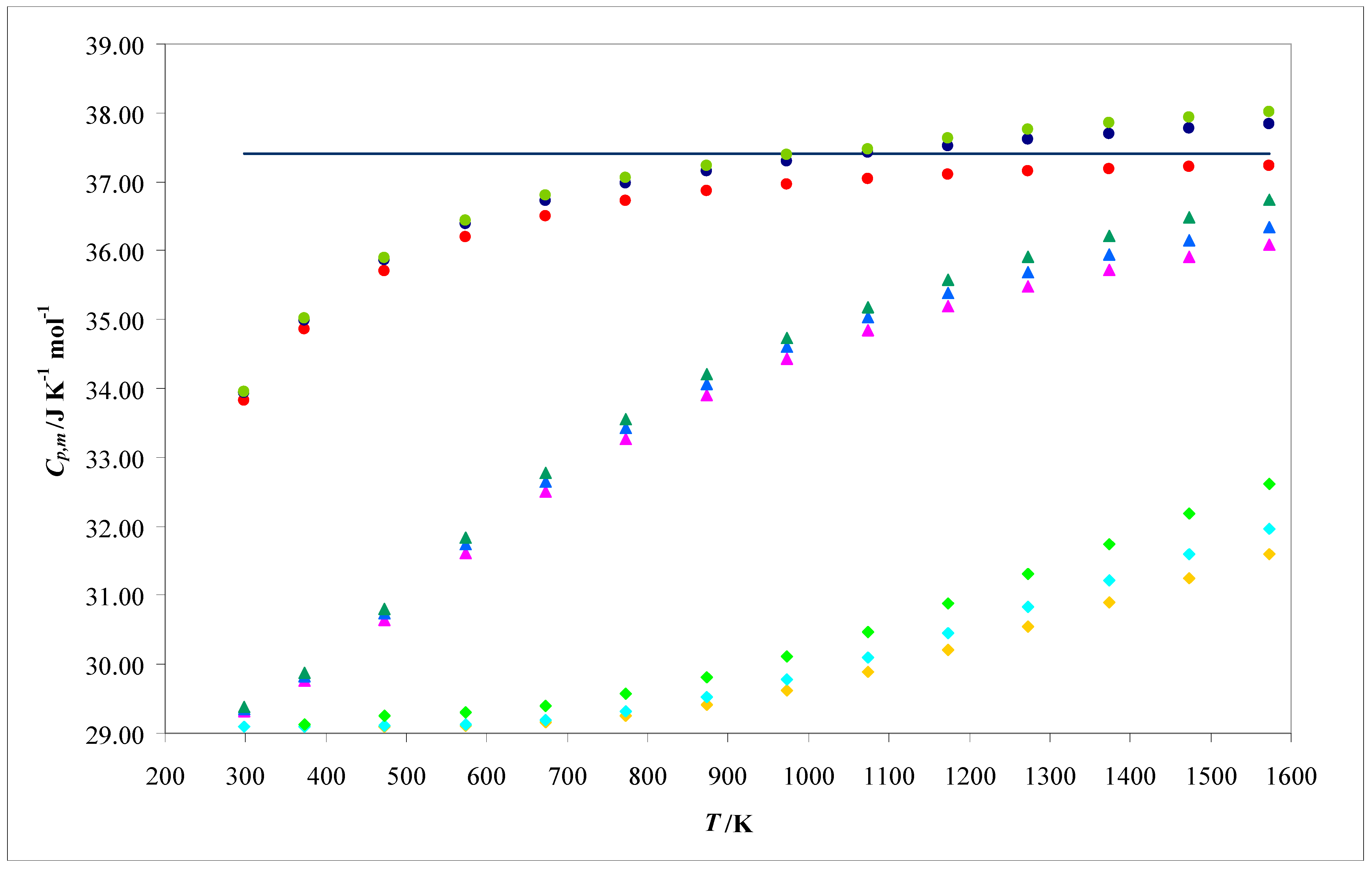
presents the corresponding values, calculated using the (Morse, class) theoretical model. Additionally, it includes the experimental values for C_p,m. In Figure 2, the calculated (using the (harm, class), (Morse, class), and (class, class) theoretical models) and experimental values for C_p,m are represented as functions of temperature.

These quantities ($T^{-2}{\sigma }_{E^{vib}}^2$ and C_p,m) are directly proportional, as can be demonstrated by combining Equations (8) and (60) for the (harm, class) theoretical model or Equations (8) and (68) for the (Morse, class) theoretical model. This way a general equation representing the referred proportionally can be obtained:

$$C_{p,m}={\displaystyle \frac{N_A}{k_B}}{T}^{-2}{\sigma }_{E^{vib}}^2+{\displaystyle \frac{7}{2}}R$$

(74)

Equation (74) is valid for both theoretical models and all the molecules since the working temperatures are significantly larger than the characteristic rotational temperatures (Θ_rot) for the molecules under study (the equipartition principle is valid for both translational and rotational degrees of freedom). This condition is fully applied in the present case, as the minimum working temperature (298.15 K) is much larger than the maximum rotational temperature (Θ_rot(H₂) = 87.46 K). In Figure 3, C_p,m is represented as a function of $T^{-2}{\sigma }_{E^{vib}}^2$. The dependence of this vibrational quantity on temperature is represented in Figure 4.

Equation (74) establishes a linear relationship between C_p,m and $T^{-2}{\sigma }_{E^{vib}}^2$. A least squares fitting, performed on these data (see Figure 3), confirmed that the respective slope and intercept are N_A/k_B = 4.36 × 10⁴⁶ J⁻¹ K mol⁻¹ and 7 R/2 = 29.10 J K⁻¹ mol⁻¹, respectively. The individual point associated with the (class, class) model, identified by the symbol in Figure 3, corresponds to the following coordinates:

$$C_{p,m}={\displaystyle \frac{9}{2}}R\iff C_{p,m}=37.42J K^{-1}{mol}^{-1}$$

(75)

$$T^{-2}\hspace{0.17em}{\sigma }_{E^{vib}}^2=\left({\displaystyle \frac{9}{2}}R-{\displaystyle \frac{7}{2}}R\right)/4.36\times {10}^{46}\iff T^{-2}\hspace{0.17em}{\sigma }_{E^{vib}}^2={\displaystyle \frac{R}{4.36\times {10}^{46}}}\iff T^{-2}\hspace{0.17em}{\sigma }_{E^{vib}}^2=1.91\times {10}^{-46}{J}^2{K}^{-2}$$

(76)

The variance of vibrational energy (${\sigma }_{E^{vib}}^2$) should reflect the Boltzmann populations for both the ground and excited vibrational states. These populations are presented in

Table 11. Boltzmann vibrational populations as a function of temperature for three representative molecules (H₂, O₂, and Cl₂), using the (harm, class) theoretical model.

Molecule	T/K	298.15	373.15	473.15	573.15	673.15	773.15	873.15	973.15	1073.15	1173.15	1273.15	1373.15	1473.15	1573.15
H2	P0	1.0000	1.0000	1.0000	1.0000	0.9999	0.9997	0.9993	0.9985	0.9973	0.9955	0.9931	0.9901	0.9865	0.9822
	P1	0.0000	0.0000	0.0000	0.0000	0.0001	0.0003	0.0007	0.0015	0.0027	0.0045	0.0068	0.0098	0.0134	0.0175
	P2	0.0000	0.0000	0.0000	0.0000	0.0000	0.0000	0.0000	0.0000	0.0000	0.0000	0.0000	0.0001	0.0002	0.0003
	P3	0.0000	0.0000	0.0000	0.0000	0.0000	0.0000	0.0000	0.0000	0.0000	0.0000	0.0000	0.0000	0.0000	0.0000
	Pv>3	0.0000	0.0000	0.0000	0.0000	0.0000	0.0000	0.0000	0.0000	0.0000	0.0000	0.0000	0.0000	0.0000	0.0000
O2	P0	0.9996	0.9979	0.9923	0.9819	0.9672	0.9489	0.9282	0.9059	0.8827	0.8592	0.8357	0.8126	0.7901	0.7682
	P1	0.0004	0.0021	0.0077	0.0178	0.0318	0.0485	0.0667	0.0853	0.1036	0.1210	0.1373	0.1523	0.1659	0.1781
	P2	0.0000	0.0000	0.0001	0.0003	0.0010	0.0025	0.0048	0.0080	0.0121	0.0170	0.0226	0.0285	0.0348	0.0413
	P3	0.0000	0.0000	0.0000	0.0000	0.0000	0.0001	0.0003	0.0008	0.0014	0.0024	0.0037	0.0053	0.0073	0.0096
	Pv>3	0.0000	0.0000	0.0000	0.0000	0.0000	0.0000	0.0000	0.0001	0.0002	0.0004	0.0007	0.0012	0.0019	0.0029
Cl2	P0	0.9312	0.8821	0.8148	0.7514	0.6943	0.6437	0.5990	0.5595	0.5245	0.4934	0.4656	0.4407	0.4182	0.3978
	P1	0.0641	0.1040	0.1509	0.1868	0.2122	0.2294	0.2402	0.2465	0.2494	0.2500	0.2488	0.2465	0.2433	0.2396
	P2	0.0044	0.0123	0.0280	0.0464	0.0649	0.0817	0.0963	0.1086	0.1186	0.1266	0.1330	0.1379	0.1416	0.1443
	P3	0.0003	0.0014	0.0052	0.0115	0.0198	0.0291	0.0386	0.0478	0.0564	0.0641	0.0711	0.0771	0.0824	0.0869
	Pv>3	0.0000	0.0002	0.0012	0.0038	0.0087	0.0161	0.0259	0.0377	0.0511	0.0659	0.0815	0.0979	0.1146	0.1315

(for the (harm, class) theoretical model) and in

Table 12. Boltzmann vibrational populations as a function of temperature for three representative molecules (H₂, O_2, and Cl₂), using the (Morse, class) theoretical model.

Molecule	T/K	298.15	373.15	473.15	573.15	673.15	773.15	873.15	973.15	1073.15	1173.15	1273.15	1373.15	1473.15	1573.15
H2	P0	1.0000	1.0000	1.0000	1.0000	0.9999	0.9996	0.9989	0.9978	0.9962	0.9938	0.9908	0.9870	0.9825	0.9774
	P1	0.0000	0.0000	0.0000	0.0000	0.0001	0.0004	0.0011	0.0022	0.0038	0.0061	0.0091	0.0128	0.0171	0.0220
	P2	0.0000	0.0000	0.0000	0.0000	0.0000	0.0000	0.0000	0.0000	0.0000	0.0001	0.0001	0.0002	0.0004	0.0006
	P3	0.0000	0.0000	0.0000	0.0000	0.0000	0.0000	0.0000	0.0000	0.0000	0.0000	0.0000	0.0000	0.0000	0.0000
	Pv>3	0.0000	0.0000	0.0000	0.0000	0.0000	0.0000	0.0000	0.0000	0.0000	0.0000	0.0000	0.0000	0.0000	0.0000
O2	P0	0.9995	0.9976	0.9915	0.9804	0.9648	0.9457	0.9241	0.9009	0.8769	0.8527	0.8286	0.8048	0.7817	0.7592
	P1	0.0005	0.0024	0.0084	0.0192	0.0339	0.0512	0.0699	0.0888	0.1073	0.1248	0.1410	0.1558	0.1692	0.1811
	P2	0.0000	0.0000	0.0001	0.0004	0.0013	0.0029	0.0056	0.0092	0.0137	0.0190	0.0249	0.0312	0.0377	0.0444
	P3	0.0000	0.0000	0.0000	0.0000	0.0001	0.0002	0.0005	0.0010	0.0018	0.0030	0.0045	0.0064	0.0087	0.0112
	Pv>3	0.0000	0.0000	0.0000	0.0000	0.0000	0.0000	0.0000	0.0001	0.0003	0.0006	0.0011	0.0018	0.0027	0.0040
Cl2	P0	0.9283	0.8780	0.8092	0.7447	0.6867	0.6353	0.5900	0.5499	0.5145	0.4830	0.4549	0.4296	0.4068	0.3861
	P1	0.0664	0.1067	0.1535	0.1888	0.2135	0.2297	0.2397	0.2451	0.2472	0.2471	0.2452	0.2423	0.2385	0.2342
	P2	0.0049	0.0134	0.0298	0.0488	0.0675	0.0843	0.0986	0.1105	0.1201	0.1276	0.1334	0.1378	0.1409	0.1431
	P3	0.0004	0.0017	0.0059	0.0129	0.0217	0.0314	0.0411	0.0504	0.0589	0.0665	0.0732	0.0790	0.0839	0.0881
	Pv>3	0.0000	0.0003	0.0015	0.0048	0.0107	0.0193	0.0306	0.0440	0.0593	0.0758	0.0933	0.1114	0.1299	0.1485

(for the (Morse, class) theoretical model).

4. Discussion

The molecular interpretation for C_p,m, as presented in this paper, is based on its linear relationship with $T^{-2}{\sigma }_{E^{vib}}^2$ (see Equations (74)–(76) and Figure 2). This indicates that both quantities exhibit analogous tendencies with respect to their variations with relevant factors such as the temperature (T) or the vibrational frequency (ν_vib). This is evident by comparing Figure 2 and Figure 4.

The temperature dependence of the aforementioned quantities (C_p,m and $T^{-2}{\sigma }_{E^{vib}}^2$) can be understood as a competition between two opposing tendencies: the increase in the variance of the vibrational energy (${\sigma }_{E^{vib}}^2$) with T and the decrease in the T⁻² term with the same variable. The overall result of this competition is that both quantities increase with T, tending to constant values at high temperatures (see Figure 2 and Figure 4). For the (harm, class) theoretical model, these limits are derived from the equipartition principle (9 R/2 for C_p,m and 1.91 × 10⁻⁴⁶ J² K⁻² for $T^{-2}{\sigma }_{E^{vib}}^2$). For the (Morse, class) theoretical model, these limits exceed those predicted by this principle. These convergences at high temperatures are evident for Cl₂ (lowest vibrational temperature: Θ_vib = 554.6 K), can be anticipated for O₂ (intermediate vibrational temperature: Θ_vib = 2999.6 K), and are not obvious for H₂ (highest vibrational temperature: Θ_vib = 6336.8 K).

The quantities under study (C_p,m and $T^{-2}{\sigma }_{E^{vib}}^2$) clearly decrease with the ν_vib (see Figure 2 and Figure 4 and Table 8, Table 9 and Table 10). This tendency originates from the decrease in the variance of the vibrational energy (${\sigma }_{E^{vib}}^2$) with ν_vib (see Figure 4).

The variance of the vibrational energy (${\sigma }_{E^{vib}}^2$) is strongly correlated with the distribution of the Boltzmann populations across different vibrational states (see Table 9, Table 10, Table 11 and Table 12). ${\sigma }_{E^{vib}}^2$ is zero when only the vibrational ground state is occupied (P₀ = 1.0000, P_v>0 = 0.0000). Promoting a more balanced distribution of the vibrational populations, by decreasing the ground state population and increasing the populations of the vibrational excited states, will increase ${\sigma }_{E^{vib}}^2$. Given the exponential nature of the Boltzmann populations (see Equations (12) and (67)), this can be achieved by increasing the temperature or decreasing the vibrational frequency (reducing the energy difference between two consecutive vibrational states). These tendencies are confirmed in Table 9, Table 10, Table 11 and Table 12.

5. Conclusions

In this paper, I presented Diatomic as an alternative to quantum chemistry packages for calculating the thermodynamic properties of diatomic molecules. Diatomic is an open-source Excel application that requires only a limited number of molecular constants to perform these calculations. In addition, these constants can be easily obtained from freely available online databases.

This new application offers two models (Morse and harmonic) to describe the vibrational structure and two models (classical and quantum) to describe the rotational structure. By combining the rotational and vibrational structures, four theoretical models can be used within Diatomic (harm, class; Morse, class; harm, quant; and Morse, quant). Diatomic presents a number of distinctive features that enable its application for different purposes.

Diatomic was used to calculate four standard molar thermodynamic properties (standard molar enthalpy of formation, molar heat capacity at constant pressure, average value of the standard molar thermal enthalpy, and standard molar entropy) for a set of fifteen diatomic molecules. The results obtained with this application were compared with experimental data.

A molecular interpretation for the molar heat capacity at constant pressure (C_p,m), as an educational application of Diatomic, was also discussed here. This interpretation utilizes certain vibrational quantities provided by this application, such as the variance of the vibrational energy and the vibrational Boltzmann populations, which are typically unavailable in general quantum chemistry packages.