Development of Trading Strategies Using Time Series Based on Robust Interval Forecasts

Abstract

The task of time series forecasting is to estimate future values based on available observational data. Prediction Intervals methods are aimed at finding not the next point, but the interval that the future value or several values on the forecast horizon can fall into given current and historical data. This article proposes an approach for modeling a robust interval forecast for a stock portfolio. Here, a trading strategy was developed to profit from trading stocks in the market. The study used real trading data of real stocks. Forty securities were used to calculate the IMOEX. The securities with the highest weight were the following: GAZP, LKOH, SBER. This definition of the strategy allows operating with large portfolios. Increasing the accuracy of the forecast was carried out by estimating the interval of the forecast. Here, a range of values was considered to be a result of forecasting without considering specific moments, which guarantees the reliability of the forecast. The use of a predictive interval approach for the price of shares allows increasing their profitability.

1. Introduction

Contemporary financial instrument management systems have information and technological support capable of collecting, storing, and processing huge amounts of data. In a broad sense, this class also includes information systems that provide information support for the Internet of Things [1], automatic production lines [2], and information support systems for government systems [3,4], but most often, it supports trading on various exchanges [5,6]. From the point of view of general characteristics, such information systems are monitoring and control systems for a multiply connected, structurally complex object, the functions of which are to analyze and visualize data [7,8]. One of the traditional approaches to multi-connected systems with many inputs and many outputs is decomposition [9], including up to the SISO level (single input–single output). In this case, the identification of this system turns out to be quite simple, but such a complex of SISO models [10] does not consider the impact to the dynamics of a particular subsystem of the structural complexity of the entire object, and it becomes difficult to compile a portfolio. Without the decomposition of a multiply connected object with hundreds of thousands of inputs and hundreds of thousands of control actions, it is impossible to adequately solve control problems; for structurally complex objects, it is necessary to develop a methodology for forming a portfolio of financial series with which it is possible to form winning investment management strategies.

Modern large information systems work with a large number of time series, making up digital analytical platforms, decision support systems, and other object management software based on predictive values. Requirements for the quality of the forecast determine the need to use forecasting models that are robust in output, that is, those that provide guaranteed upper and lower estimates. The currently existing PI (Prediction Intervals) methods [11] are able to provide the requirements for the quality of time series forecasting.

Time series forecasting is an important problem in scientific research with a wide range of practical applications, including economics, environmental sciences, energy, and more [12,13]. In a general sense, a time series is a sequence of observations of some system or phenomenon in chronological order. The task of time series forecasting is to estimate future values based on available observational data. Time series forecasting is a traditional research topic in statistics, econometrics, and related fields [14]. The range of methods is quite wide (see Table 1 in [11]), spanning from autoregressive methods such as ARIMA to modern methods using artificial neural networks and machine learning, fuzzy logic, etc. The advantages of traditional one-dimensional methods are that they can work with a minimum amount of data; however, such approaches to time series modeling take into account only the features and patterns inherent in one time series without taking into account the structural complexity or portfolio of time series [15].

PI methods are aimed at finding not the next point, but the interval in which a future value or several values can fall on the forecast horizon under the given current and historical data. As is known, up to a certain point, interval analysis [16] develops, but it simply ceases to have a physical meaning even when solving linear algebraic equations, encountering the operation of multiplying intervals. In the theory of PI, there is no multiplication operation; only the addition of intervals is introduced. The use of PI provides a decrease in the degree of uncertainty in the data and the robustness of the model in terms of output, but at the same time, the accuracy of the forecast is also blurred. A guaranteed hit in each forecast interval is a reduction in error, and with a sufficiently wide interval, there is a complete exclusion of error.

This article proposes an approach to modeling a robust interval forecast for a portfolio of stocks. A trading strategy was developed to profit from trading stocks in the market. The study used real trading data of real stocks. To calculate the Moscow Exchange Index (IMOEX), 40 securities were used. The securities with the largest weight were GAZP, LKOH, SBER. First, we used the well-known method of dividing the time series into trend, cyclic, and noise components. Based on the stock price forecast, we determined the entry point strategy to be in an open position for most of the trend movement. The optimal points for opening and closing positions are located at the points of the local extrema of the cyclic component. This definition of the strategy allows you to operate with large portfolios. Increasing the accuracy of the forecast was carried out by estimating forecast intervals. When calculating PI, we removed uncertainties, ensuring that local extrema fell within the calculated range. The main problem of this strategy is that false positives on small fluctuations do not lead to local turning points, whereas using intervals guarantees insensitivity to noise. An important feature of the interval forecast is the forecast of a limited tube: we obtained a forecast both for a given width (forecast horizon) and for a given height at each predicted point. For the problem under consideration, we used the ranges of values bounded by a rectangle as an interval.

The contribution of the article is as follows:

• We considered, as a result of forecasting, a range of values without taking into account specific points, which guarantees the robustness of the forecast.
• We developed a method for modeling the stock price in the form of a range, which ensures the insensitivity of the model to local noise.
• We used the predictive intervals approach to predict the stock price when managing a portfolio, which allowed us to increase profitability.

The structure of the rest of the article is as follows. Section 2 contains analyses of background studies and provides basic information about the interval forecast and the algorithm for constructing the PI. Section 3 describes the research methods and initial data for modeling. Section 4 reports the results of building effective strategies; here, it is demonstrated that when using inaccurate models, combining their intervals makes a profit based on the analysis of PI. Section 5 contains the conclusion and suggestions for further research.

2. Background

As you know, the price of an individual stock fluctuates more often due to its dynamic, non-linear, non-parametric, and chaotic properties. Although it is difficult to predict individual stocks, given the many uncertainties in the stock market, many studies are still developing patterns in stock trends, and there is a reason for this. Many researchers have shown that available information is accumulated and reflected in prices and in historical data. That is the nature of the market: the general trends that occur are all reflected in historical price change data. By identifying changes inherent in stocks, you can evaluate the forecast of future values. Approximately 90% of large stock traders use the time series forecasting method based on the trend model [7]. Other researchers have sought to predict stock market trends through sophisticated means. There is research based on the news, finding correlations between the news and the actions of traders in relation to stocks. Regulators have a significant influence on stock indices. However, stock trend forecasting approaches are sensitive to minor factors.

Currently, there are several applied areas in which PI is used, for example, in wind forecasting [17] and solving energy problems [18]. Despite the large number of works on the topic of PI, it is not generally accepted; thus, it is necessary to explain some features of this approach.

The intervals have always been incorporated into some methods; in all methods of using statistics, there are always confidence estimates. In regression models, the confidence interval is an integral part of these models, but not everyone pays attention to it. Intervals can also be seen in the methods of the Gaussian process: fuzzy variables are set in intervals, and intervals can occur in conditions of inaccurate measurement of parameters. However, in all of these methods, unlike in PI, there is no task to reduce or expand the intervals. A distinctive feature of PI is obtaining guaranteed ranges of predicted data estimates.

One of the key methods is a nonparametric method for finding estimates of the lower and upper bounds of the PI, which is called LUBE (Lower Upper Bound Estimation) [19]. The implementation of the LUBE approach aims to build the PI directly from the input without any additional assumptions about the distribution of the data. The LUBE method was proposed in [20] and is aimed at constructing narrow most probable ranges of PI, posing an optimization problem in which the introduced criteria for evaluating the quality of solutions are used as the objective function. The most common problem is the two-criteria problem of finding a compromise. For example, in [21], the Pareto set is searched using evolutionary calculations.

The two most used indices are PICP and PINAW.

Let there be a time series representing forecast values for the horizon N: Y = {y₁, …, y_i, …, y_N}.

PICP is a score index for PI that indicates the likelihood that future values will be inside the lower and upper bounds [22]:

$$\mathrm{PICP}=\frac{1}{N}{\displaystyle \sum _{i=1}^N{a}_i},$$

(1)

where N is the size of the data sample, and a_i is a binary variable defined by the formula:

$$a_i=\{\begin{array}{l}1,\hspace{0.17em}{y}_i\notin [y_{i-},\hspace{0.17em}{y}_{i+}];\\ 0,\hspace{0.17em}{y}_i\in [y_{i-},\hspace{0.17em}{y}_{i+}].\end{array}$$

(2)

In Equation (2), the values $y_{i-}$, $y_{i+}$ are estimated lower and upper bounds. To ensure the accuracy of the PI, it is usually required that the PICP exceed a predetermined confidence level. In this study, the forecasting method allows 5% exits for the forecast interval.

PINAW is introduced to assess the effectiveness of PI [21]:

$$\mathrm{PINAW}=\frac{1}{N\cdot W}{\displaystyle \sum _{i=1}^N(y_{i+}-y_{i-})},$$

(3)

where W is the width of the range of PI values. The goal is to minimize the PI width.

Other indices are also possible [11], and they form the optimization problem with the aim of obtaining intervals.

We illustrate with a simple example using an accessible and well-known dataset of the S&P 500 index with a daily value at the close of trading.

We applied the traditional decomposition into seasonal components and built predictive ARIMA models in the form of intervals using Colab. Figure 1 shows the interval predictive models for the seasonal component, trend, and noise.

Thus, there are three series, and for each one, it is possible to build its own interval model. The noise component serves for fast predictions, and given the uncertainty, it provides a wide enough range to provide good PI. It allows the use of narrow intervals for a trend chart. The peculiarity of the author’s approach lies in the following algorithm. At the first step, we built several “simple” models (such as moving averages) without adjusting the models for accuracy because such adjustments provide interpolation, not forecast quality. The second step of the algorithm is the construction of intervals around the predicted values. The third step is interval pooling, which consists of using the maximum upper and lower bounds [11] of all used “simple” models. The fourth step is to reduce the interval as a solution to the optimization problem according to criteria (1)–(3). Thus, considering the monotonicity and smoothness of the trend component, it is possible to provide an interval forecast with a guaranteed level of accuracy.

3. Methods

Classic trend strategies are very popular when working with stock, commodity, and currency markets. Their essence is to divide the time series of market quotes into trend, cyclic, and noise components, and then to determine the optimal points for opening a position to be in an open position for most of the trend movement. It means to, despite the noise component, open a position in the direction of the trend component and close it exactly at the extremes of the cyclic component. Figure 2 clearly shows two trends, a downtrend and an uptrend, as well as fluctuations in the cyclical component. In this figure, there are no pure trends, and the price always oscillates around the trend. Strong fluctuations, with the wrong choice of the optimal position opening point, can neutralize a significant part of the trend movement. The optimal points for opening and closing a position are exactly at the extremes of the cyclical component. It means one should sell as high as possible and buy as low as possible. For example, the uptrend in Figure 2 starts at the local minimum of the cyclical component at the trend reversal to open a position up, and the local maximum of the cyclical component is at the end of the trend, where one should close the position.

Here, it is necessary to understand how prices will move on an uptrend. Two types of growth can be distinguished: a small jump or a rise leading to a local extremum. We understand a local extremum as a change in the sign of the first derivative at an inflection point on a trend or cyclic component (turning point).

Figure 2 shows the IMOEX chart for the period July 2020–February 2021. This is the “Japanese candlestick” chart, the most common among traders at the moment because it gives in a compressed form the most complete picture of the dynamics of the exchange price from a given discretization. The chart consists of rectangles with tails, or the body of the candle and its shadows. Each individual element is the fluctuations of quotes for a certain period of time, which is called a timeframe. On this chart, the timeframe is 1 day. The end point of the upper tail is the high price for 1 day, the lower tail is the low price for this day, the red candlestick represents that the closing price of the day was below the opening price, the green one represents that the closing price of the day was above the opening price, and the closing and opening prices are the borders of the rectangle. It is very similar to the speckled box-and-whisker chart from the standard set of charts in Excel. Regarding the parameters of each candle, the following terms are used hereafter on these charts: open (O)—the opening price; close (C)—closing price; low (L)—minimum value; high (H)—maximum value.

The global inflection points in Figure 2 happened on 14 August 2020, 30 October 2020, and 12 January 2021. Their difference from smaller fluctuations, noise, is that the trend component demonstrates monotonicity to forecast depth. Monotony can decrease or increase. The task is to determine the forecast in the form of an interval and to identify the inflection point of the trend. Shown in the region of November 1–3 is uncertainty, where the trend can either go up or continue to decline.

The main advantages of trend strategies are as follows:

−

simple in terms of technical implementation, unlike various scalping techniques, pair trading, counter-trend strategies, etc., and trends can be tracked visually;

−

understandable for most investors: “bought low, sold high”;

−

most importantly, they allow operating with large portfolios, which differs from the same scalping; in fact, the portfolio is determined by the volume of the market.

The main disadvantages of trend strategies stem from the principles of their construction and market dynamics. “Pure” trends, which can be profitable, are less common than cyclical and noise components. For a trend strategy, it is extremely important to correctly and timely detect a trend and extract maximum profit from it while allowing a minimum number of losing trades due to false signals, which, as a rule, will be more frequent, and minimizing losses on them.

Automated trend strategies are implemented through the analysis of the time series of quotes using digital filters. These are either popular technical indicators of trading terminals (MA, MACD, RSI, etc.; the essence is simple digital filters) or more complex digital filtering and machine learning algorithms.

Consider the simplest classic trend strategy: the intersection of simple moving averages. Based on the time series of closing prices, two simple moving averages were built:

$${\mathrm{M}\mathrm{A}}_{\mathrm{t}}\left(n\right)=({\mathrm{C}}_{\mathrm{t}}+{\mathrm{C}}_{\mathrm{t}-1}+\dots +{\mathrm{C}}_{\mathrm{t}-\mathrm{n}})/n$$

One moving average is “short” with a period of n, and the other moving average is “long” with a period of m > n. Further, in the following examples, n = 10 and m = 25. Crossing the “short” moving average “long” from the bottom up is a signal to open a long position and close a short position, and from top to bottom, it indicates one should close a long position and open a short position.

Hereinafter, we use the Moscow Exchange Index, IMOEX, with a period of 1 day as a traded instrument.

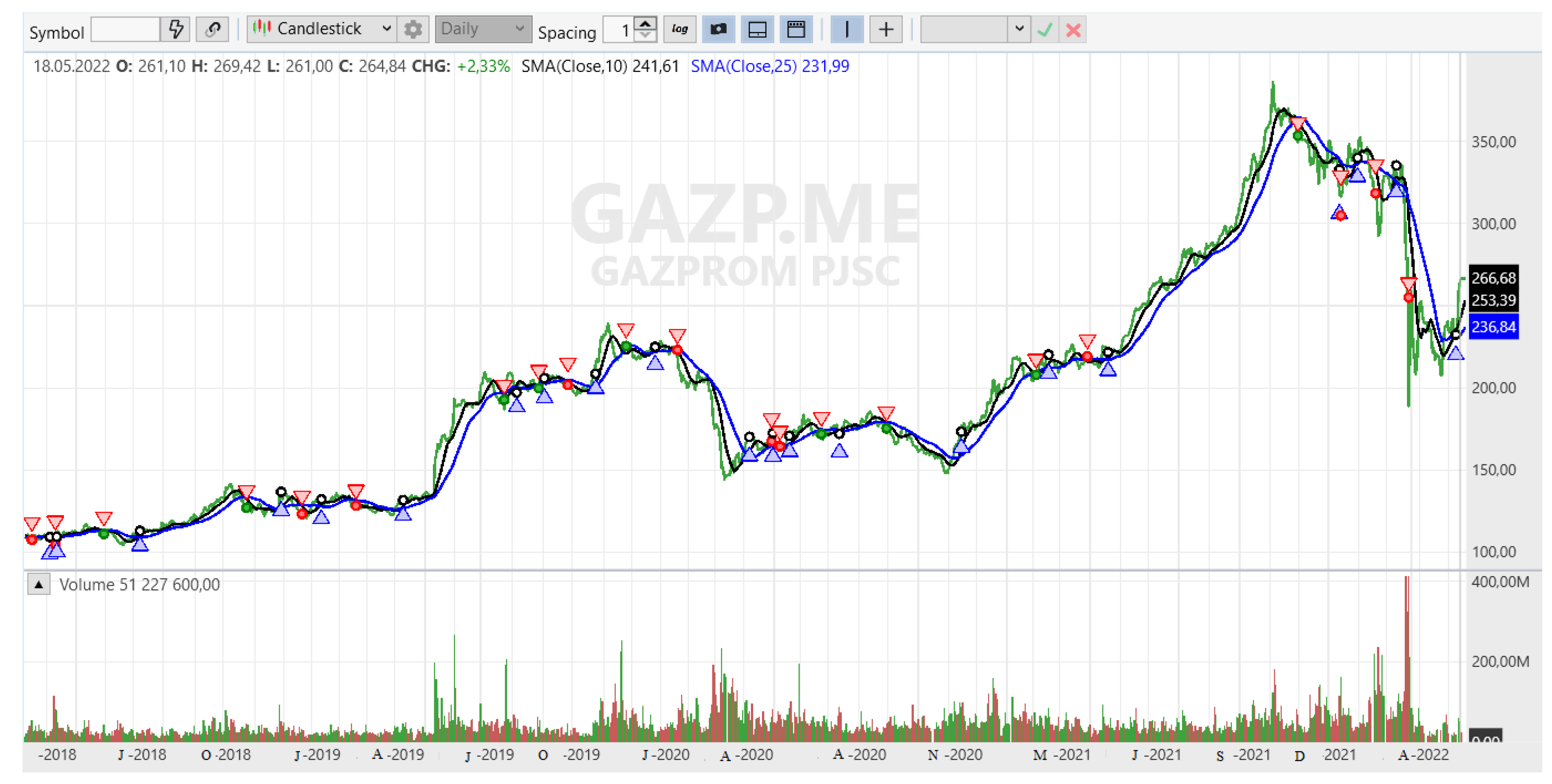
Figure 3 shows the main problems of trend strategies. There are delayed signals for opening and closing positions; the crossing of moving averages, like any other filters, occurs with a delay. There are also false positives during periods of no trend and increased volatility.

Figure 3 shows a 1-year range from 1 July 2021 to 31 June 2022. Here, 2 simple moving averages (MA) with periods of 10 (orange, more “fast”, line) and 25 (green, “slow”, line) are superimposed on the price chart that we discussed previously. Intersection points are labeled.

Figure 3 clearly shows that the delay of position opening signals relative to the optimal entry and exit points, even on such pronounced trends with minimal volatility of the cyclical component, will lead to a loss of about 20–30% of the trend movement (blue areas). In addition, in the case of a sideways trend and a period of increased volatility (the pink section), the trend strategy will give many false signals.

Various methods are used to solve these problems. In particular:

−

Applying more advanced filters to reduce latency. However, it will still exist [23,24].

−

Periodic selection of more optimal filter parameters. However, the statistics of several prices still change unpredictably.

−

Selection of robust filter parameters to eliminate false positives and the need for periodic reconfiguration of the filter is the essence of a spark-robust solution to multicriteria optimization. However, the profitability of the strategy will then trend to zero.

To solve the problems of trend strategies, it is proposed to use robust interval models for predicting structurally complex systems such as those described in [11].

Instead of fighting for the selection of optimal parameters at the input, it is proposed to consider the principle of robustness at the output.

Thus, it can be convincingly shown that noise is included in the PI; thus, it is enough to decompose the original series into cyclic and trend components. This makes it possible not to separate the two types of noise. The first type is noise that has arisen as oscillations of phase trajectories around the limit cycle or chaotic dynamics. The second type of noise is related to the nature of the trend. Eliminating model uncertainty by guaranteeing a given forecast quality provides a new set of tools for investor decision-making. The PI increases the robustness to input fluctuations, ensuring that the uncertainty in the output is eliminated.

To calculate the Moscow Exchange Index, IMOEX, 40 securities were used. The securities with the largest weight were GAZP (14.28%), LKOH (12.72%), and SBER (13.16%), according to the data from www.moex.com as of 20 January 2023. As can be clearly seen in Figure 4, there is a significant correlation between the securities included in the index (orange line—SBER, turquoise—GAZP, yellow—LKOH) and the index itself. This is especially evident in time series with a period of 1 day or more. This is explained by the peculiarities of the securities included in the index and by the fact that during the day, the key news affecting the market already has time to be considered, and its price may already vary. However, even despite this, the chart shows that the key trend reversals for individual securities and the index occurred at different points in time. For example, in Figure 4, these areas are highlighted with pink rectangles. On the candlestick chart in the period of 1 h, the situation would be brighter.

Accordingly, if we analyze the securities separately and take all of the signals from the securities included in the index as signals for opening a position, we will get the result shown in Figure 5. Signals for opening a position will appear around the optimal position entry points. Some will appear earlier, and some will appear later. If, at this moment, positions are opened, for example, in equal shares, then the entry point to the position will be as operative as possible and as robust as possible with respect to noise and cyclic components.

In addition, periods of index volatility will reflect periods of volatility for securities included in the index. However, some securities during the period of volatility will have a pronounced trend (Figure 6). Accordingly, there will at least be no more false positives during the period of volatility than if we had simply analyzed the index series.

It does not matter what filters we use for each stock separately. With enough rows included in the final index, we get a robust trend strategy.

4. Results

We conducted simple computational experiments to show the advantages of trend trading strategies based on PI calculation approaches.

As a starting point, we took the simplest trend strategy: the intersection of simple moving averages with periods of 10 and 25. We only opened long positions when MA (10) > MA (25), and we closed when MA (10) < MA (25). We opened a position at 80% of the available liquidity, and we analyzed series with a period of 1 day.

We applied the strategy for time series with a period of 1 day for GAZP, LKOH, and SBER (Figure 7, Figure 8 and Figure 9). In the figures: blue triangles are signals to buy and open a long position; red triangles are signals to sell and close a long position. Dark green parts of the chart are periods when the system opened a position, and light green parts are periods when the system did not open positions, holding cash instead. Accordingly, the chart shows that the profit curve grew (or fell if the signal turned out to be false) in dark green areas and remained unchanged in light areas.

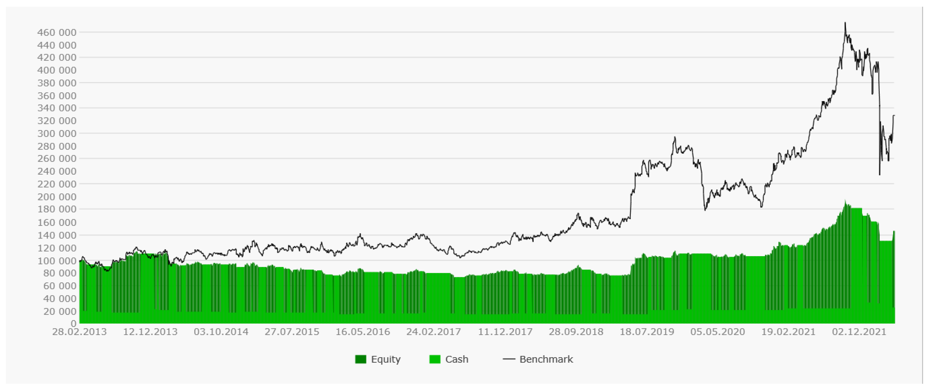
As can be seen from the profit curves (see Figure 10, Figure 11 and Figure 12), for each of the securities, the trend trading strategy based on two moving averages is rather suboptimal. Despite the rather significant movements in the securities, the profits managed to extract quite a bit. For comparison, next to the profit curve is the price curve of the stock itself (benchmark). It means that if at the initial moment, we had just bought the stock for all available liquidity, the profit curve would repeat the curve of the stock with all of its ups and downs, of course, but nevertheless, the yield would be significantly higher.

However, significant trends, albeit with a significant delay, were identified, and there were few false signals. Profit curves ascended without drawdowns. This is perhaps the only plus of our suboptimal conservative strategy. The profit curve’s rises were very limited (dark green areas). The strategy parameters were selected with a large margin of robustness, and we missed most of the trend due to delays; however, the system held its money and did not open a position on downtrends (light green areas).

At this point, we complicated the strategy.

We analyzed all of the same time series with a period of 1 day for GAZP, LKOH, and SBER securities, but in aggregate as a portfolio. We evaluated the dynamics of an already structurally complex system. These stocks do not fully describe the index, but they are a significant part of it. Even despite this significant assumption, the analysis of each security separately and the subsequent aggregation of the forecast into a single forecast made it possible to sharpen the prediction interval in which all values of the index will fall.

We analyzed trading signals for each security, but we opened a position on the index itself in equal shares of 33% of 80% of the available liquidity as signals appeared. For those, we traded the index according to the output of the robustness model.

As mentioned previously, around the optimal entry points to the position, trading signals appeared, which were obtained because of the analysis of each of the rows. Figure 13 clearly shows the downtrend, uptrend, and lateral trend identified by the strategy. Setting up a position in equal shares of 33% on the blue marks provided an ideal diligent entry point into the position, exactly like closing a position in equal shares on the red marks.

All values of the time series of the index turned out to be within the specified intervals, despite all the assumptions with the number of time series describing the structurally complex index and the quality of the forecasting models for each of the series.

The moments of the appearance of the trading signals were the same as in Figure 10, Figure 11 and Figure 12. However, the profitability curve of the strategy was different. As can be seen from the graph (see Figure 14), the profit is significantly higher. As a benchmark, the price curve of the most profitable of the three stocks, SBER, is given. The system was almost always in a state of open positions. This is explained by the fact that we caught all of the movement along the trend more clearly.

In addition, the strategy itself and its money management can be built more comprehensively, relying not only on a robust forecast, but also on reliable boundaries of the upper and lower intervals.

5. Conclusions

The management of the financial instruments of the stock market is based on forecasts. Modern market forecasts are about 60% accurate [7], which increases the risk of investment. To form a portfolio, a set of slow-changing, low-yield stocks and fast-changing, high-yield stocks is often used, thereby reducing risk.

This article proposes an approach to forecasting in the form of forecast intervals. PIs have proven themselves well as predictors of rapidly changing complex parameters, such as wind dynamics. The advantage of PI is that noise is included in the interval model; thus, it is enough to decompose the original series into cyclic and trend components. This makes it possible not to separate sources of noise, including (1) noise that arises as oscillations of phase trajectories near the limit cycle or chaotic dynamics, and (2) noise associated with the nature of the trend. PI increases the robustness to input fluctuations, ensuring that ambiguity in the output is eliminated.

The decision-making strategy is defined as follows. Based on the stock price forecast, the position opening points are made in such a way to be in an open position for most of the trend movement. The optimal points for opening and closing positions are located at the points of the local extrema of the cyclic component. When calculating PI, we removed uncertainties, ensuring that local turning points will fall within the calculated range. To predict prices, ranges of values bounded by a rectangle were used as intervals.

To calculate the Moscow Exchange Index, IMOEX, 40 securities were used. The securities with the largest weight were GAZP, LKOH, SBER. In this article, it is shown that the approach to the definition of a robust output model based on the analysis of series, which describes a structurally complex system, gives good, stable results, even under significant limitations.

It is also shown that robust interval forecasts are understood for the investor, eliminate uncertainty, and increase insensitivity to small fluctuations.

It is possible to increase the accuracy of the forecast and, accordingly, the profitability of the strategy in several ways.

The first, and most obvious, is top open not only long positions, but also short positions.

The second is to apply more advanced forecasting algorithms rather than simple moving averages. This could include, for example, filters such as AMA, FRAMA, JMA, or others.

Third, one can take into analysis not only the three main securities of the index, but also all of the securities that form it.

The fourth is to switch to the analysis of candles of a smaller period, such as hourly or fifteen-minute candles, and continue to conclude transactions at the prices of daily candles. You can, in principle, go down to analysis of individual ticks of the exchange price.

Fifth, one can choose an entry point not at the moment of receiving a trend reversal signal. In the given example, the moment of MA crossing was chosen, but the moment when the price rebounded from the lower boundary of the robust forecast interval would allow us to get a slightly more optimal entry point.

The sixth is to supplement the strategy with the basic elements of trend strategies, such as moving stop–loss, dynamic position acquisition, and regular re-optimization of parameters according to a sliding scheme.