Abstract
Although the full form of the Rayleigh–Plesset (RP) equation more accurately depicts the bubble behavior in a cavitating flow than its reduced form, it finds much less application than the latter in the computational fluid dynamic (CFD) simulation due to its high stiffness. The traditional variable time-step scheme for the full form RP equation is difficult to be integrated with the CFD program since it requires a tiny time step at the singularity point for convergence and this step size may be incompatible with time marching of conservation equations. This paper presents two stable and efficient numerical solution schemes based on the finite difference method and Euler method so that the full-form RP equation can be better accepted by the CFD program. By employing a truncation bubble radius to approximate the minimum bubble size in the collapse stage, the proposed schemes solve for the bubble radius and wall velocity in an explicit way. The proposed solution schemes are more robust for a wide range of ambient pressure profiles than the traditional schemes and avoid excessive refinement on the time step at the singularity point. Since the proposed solution scheme can calculate the effects of the second-order term, liquid viscosity, and surface tension on the bubble evolution, it provides a more accurate estimation of the wall velocity for the vaporization or condensation rate, which is widely used in the cavitation model in the CFD simulation. The legitimacy of the solution schemes is manifested by the agreement between the results from these schemes and established ones from the literature. The proposed solution schemes are more robust in face of a wide range of ambient pressure profiles.
1. Introduction
Cavitation is a phase transformation from liquid to vapor due to a pressure drop. When the pressure in the liquid drops below a threshold, nuclei suspended in the liquid will grow to microbubbles due to vaporization. These bubbles implode under a recovery pressure, releasing a great amount of energy in the form of microjets, shock waves, and heat. The violent implosion of bubbles is mostly viewed as a negative effect in engineering systems to be avoided. The implosion of bubbles may corrode the material and may cause unwanted vibrations and noise. Meanwhile, the energy release by bubble implosion may also be exploited in some scenarios such as emulsification processes, surface treatment, and particle dispersion. Whether avoiding the negative effects of cavitation or exploiting its positive effects, insight into the bubble dynamic calls for robust models which govern the bubble growth and collapse.
The Rayleigh–Plesset (RP) equation is definitely a milestone of establishment of a cavitation model and has been manifested to be legitimate by extensive experiments. It governs the bubble growth and collapse, which occur in response to the ambient pressure and temperature. The RP equation is derived from the Navier–Stoke equation and continuity equation under the assumptions that the bubble remains spherical, the fluid is incompressible, and homogenous pressure fields prevail outside bubbles. The thermal effect on bubble response, which has been demonstrated by extensive experiments [1,2,3,4,5,6,7], can be incorporated by the RP equation, but it calls for coupling with the heat equation. The RP equation in this study assumes the isothermal condition and is given by Equation (1). It is a highly non-linear second-order ordinary differential equation of the bubble radius. A schematic diagram of the bubble modeled by the RP equation is shown in Figure 1.
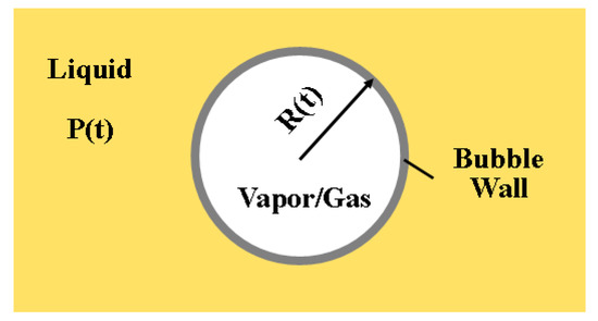
Figure 1.
Schematic Diagram of a Bubble in Liquid Molded by the RP equation.
There are various numerical methods of modeling and simulating multiphase fluid systems. Some of the methods such as the central-type space–time schemes are aimed at overcoming computational stability and computational efficiency [8,9]. One of classic methods is to treat the multiphase fluid as a mixture and solve the conservation equations of the mixture. In this method, the transport equation of the phase volume fraction is added to close the solution. The Rayleigh–Plesset equation is developed as the cavitation model by Singal et al. [10], Zwart et al. [11], and Schnerr-Sauer et al. [12] and serves as the keystone for this transport equation. These cavitation models mainly use a reduced form of the RP equation where the acceleration, gas, and viscous and surface tension terms are neglected. A so-called Rayleigh Solution Equation (2) derived from this reduced form is converted as the source or sink term of the mass transfer rate between phases in the transport equation. In the Singhal model [10], two empirical coefficients are included in the source or sink term to calibrate the evaporation and condensation rate. These two coefficients were proved to be generally valid for various flow conditions. The Zwart model [11] and Sauer model [12] use different mass transfer terms, but their terms share the common groundwork—that is, Rayleigh Solution. Variants of these types of cavitation models that only consider the pressure-driven term are discussed in Owis et al. [13], Bakir [14], Deimel et al. [15], and Bicer et al. [16].
Since the foregoing cavitation models only keep the linear term and pressure term, they are robust and stable in various scenarios of cavitating flow when they are coupled with the Volume of Fluid method to solve the phase transport equation. Their robustness and stability, which are manifested by extensive numerical studies on the cavitating flows, facilitate their application in CFD analysis. Such simplification of the RP equation sustains in certain cases of cavitation development. For example, in the late stage of bubble growth where the bubble size is relatively large. However, the significance of the ignored terms, such as the acceleration term, gas term, surface tension term, and viscous term, need to be reassessed. In the study of evolution of bubbles generated by laser ablation, Soliman et al. [17] discovered the significance of the surface tension and the liquid viscosity when they compared the radius of the bubbles obtained experimentally and numerically. Ye et al. [18,19] found out that bubble growth rate was greatly reduced when the bubble–bubble interaction and second-order derivative term (acceleration term) were considered. Žnidarčič et al. [20] also reported the significance of the acceleration term in bubble growth and collapse when the pressure rapidly changes. Lomakin et al. [21] studied the effects of contaminant gas content on cavitation intensity in the centrifugal pump with a three-phase model. Their results showed that cavitation intensity increased with the gas content, which is beyond the capability of the Schnerr–Sauer model. In fact, some researchers have calibrated or modified the Rayleigh solution-based cavitation model case by case to compensate for the simplifications. Deimel et al. [15] and Bicer et al. [16] calibrated empirical numbers in the cavitation model or added a coefficient to the pressure-driven term to tune the bubble growth and collapse rate for their specific case.
The benefits of solving the full form of the RP equation are clear compared to using the simplified Rayleigh Solution, but the full form of RP poses challenges related to the stability of the solution. A large variation of the ambient pressure leads to a rapid change in bubble radius, prompting the stiffness issue of the RP equation. The stiffness issue caused by a rapid reversion of the bubble wall movement in the rebounding phase may lead to numerical solution instability. The solution stability calls for tiny time steps. Using the adaptive time step is a valid solution strategy to compromise between numerical solution stability and computational cost. Shams et al. [22] employed a fine time step at the singularity point of the bubble radius to ensure stability and a large time step for the rest of the portions to reduce computational time. The fine time step works when the pressure variation is large and the initial bubble size is small. Alehossein et al. [23] developed a finite difference model for a cavitating nozzle. An adaptive time-step technique was applied, and the modified Euler method equipped with this technique successfully solved the RP equation for wide ranges of pressure variation and bubble initial sizes with high efficiency. In their method, the time step was dictated by the change in the ratio of bubble radius between adjacent steps.
By employing different time steps for singular and non-singular portions of the solution, the scheme equipped with the adaptive time-step technique ensures its stability with less computational cost compared to solution schemes which employ constant time steps. However, it is confronted with some limitations, especially in the framework of engineering application and CFD analysis. The slow advance in time at the singularity point of the RP equation is time-consuming and may not be cost-effective for the CFD software packages. The time step used at the singularity point of the RP equation may be incompatible with the convergence criteria of other fluid dynamics equations, which may require using fine time steps, thus increasing computational cost. Another possibility is that the coarse time step used in non-singular proportions may have to be refined to comply with the convergence criteria of other equations, making the adaptive time-step technique less attractive.
This study aims at solving the full form of Rayleigh–Plesset equation for better accuracy, even if the bubble undergoes a steep pressure variation. Distinguished from the adaptive time-step strategy, the proposed scheme tackles the stiffness issue via an approximation of the minimum bubble size in the collapse stage and can tolerate a time step dictated from somewhere else. This makes it more compatible with time marching of other conservation equations. The specific objectives are to (a) develop the robust solution scheme for RP equation, which is given by Equation (1) when the isothermal condition is assumed, (b) solve the RP equation for the bubble radius under various types of the ambient pressure and prove the legitimacy of the proposed solution schemes by comparing their results with published work, and (c) analyze the convergence of the proposed solution schemes by varying the time step size.
2. Solution Strategy and Discretization of Equations
The bubble wall velocity at the final stage of collapse is so high that a coarse time step results in a misleading estimation of the minimum bubble radius, which may be even negative. Subsequent to the minimum bubble radius, the gas inside the bubble that is substantially compressed in the collapse stage will rapidly reverse the bubble wall velocity. Change in the bubble radius in this period causes the singularity or stiffness issue and therefore is where the adaptive time-step technique refines the step size. Both solution schemes presented in this study employ a truncation bubble radius to approximate the minimum bubble radius when the calculated one is negative. Meanwhile, the time step size is set as a constant. The first scheme employs the finite difference method and prediction–correction method to solve the RP equation for wall velocity and bubble radius. It is therefore referred to as the FD PC algorithm. The second scheme employs the Euler method to solve for the wall acceleration, wall velocity, and bubble radius. It is referred to in this study as the Euler algorithm.
The proposed scheme can be coupled with the transport equation of the vapor phase (Equation (3)) to solve for the cavitation in the CFD software packages. As summarized in the introduction, the current cavitation models used in the CFD software, such as the Singhal model [10], Zwart model [11], and Schnerr–Sauer model [12], calculate the mass transfer rate between the liquid and gas phases (Equations (4) and (5)) from the reduced form of the RP equation (Equation (2)). Equations (4) and (5) indicate that the mass transfer rate, either vaporization or condensation, is a function of the wall velocity, which is derived from the reduced form, and the vapor volume fraction. As the reduced form of RP equation excludes the effect of the second order term, viscous term, and gas term, the bubble growth and collapse rate are either overestimated or underestimated [17,18,19,20,21].
2.1. Finite Difference Prediction–Correction Scheme (FD PC Algorithm)
The finite difference prediction–correction scheme (FD PC Algorithm) explicitly solves for the wall velocity. In this scheme, the RP equation is transformed, and the procedure is divided into two steps—the prediction step and correction step. As shown in Equation (6), the left side of the RP equation (Equation (1)) is transformed to the first derivative of a function of the bubble radius and bubble wall velocity. The viscous term is excluded first, and the bubble wall velocity is predicted. Subsequently, the bubble wall velocity predicted in the previous step is corrected by introducing the viscous term back.
In accordance with the prediction and correction step, the bubble wall velocity is decomposed into two parts as shown in Equation (7): (i) , which is predicted without the viscous term, and (ii) , which is used to correct by taking into account the viscous effects. The governing equation for and are given by Equations (8) and (9), respectively. Equation (9) can be rewritten as Equation (10) by plugging Equation (7) into it. As a result, solving the RP equation becomes equivalent to solving Equations (8) and (10) in sequence.
The proposed solution scheme adopts the finite difference method and is established on the discrete form of Equations (8) and (10). Using the backward and forward difference method, Equation (8) ends up as Equation (13) after a series of transformations shown by Equations (11) and (12). Meanwhile, using the backward difference method, Equation (10) can be temporally discretized as Equation (14) to calculate .
The flowchart of the proposed solution scheme is shown in Figure 2. After inputting the known variables such as the ambient pressure and initial conditions, the prediction and correction steps are carried out in sequence using Equations (13) and (14). If the bubble radius at the current time step is smaller than a threshold , which is set as a small value, correction of the bubble wall velocity is made. Otherwise, no correction occurs. This is because the viscous term mainly dominates the bubble behavior in the collapse stage, where the bubble is tiny and wall velocity is considerable, rather than in the growth stage. After the bubble radius of the next time step is calculated from the bubble radius and wall velocity of the current time step, this new bubble radius is filtered by a near-zero truncation radius to ensure it is non-negative. A negative bubble radius may occur when the time advances too aggressively at the final stage of bubble collapse. When a negative bubble radius occurs, it is replaced with the minimum bubble radius and the bubble wall velocity is correspondingly updated based on .
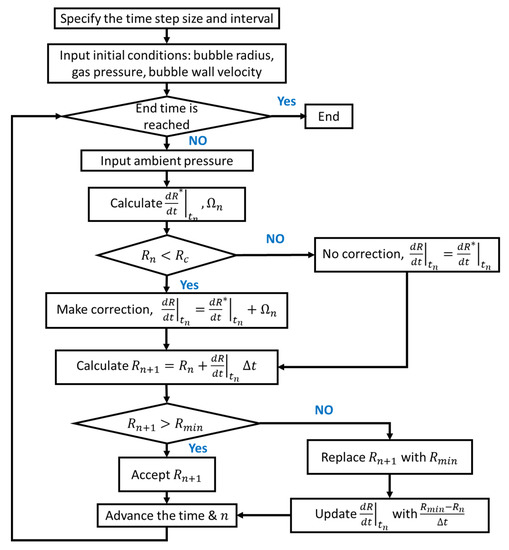
Figure 2.
Flowchart of FD PC Algorithm.
2.2. Euler Method-Based Scheme (Euler Algorithm)
In the Euler method-based scheme (Euler Algorithm), the RP equation is cast into a system of two first order ODE equations (Equation (15)). The variables and in (15) represent and , respectively. Based on the Euler method, the discrete form of and are derived as Equations (16)–(18). As shown in the equations above, this scheme is a 2nd order method which computes twice for . The variable is computed the first time and is computed the second time. Meanwhile, the ambient pressure of the next time step needs to be input in this scheme. In contrast, the FD PC algorithm is a 1st order scheme and only requires the ambient pressure of the current time step, .
The flow chart of the Euler Algorithm is shown in Figure 3. If the is less than the truncation radius, , it is replaced by and the current states of bubble including the wall velocity are correspondingly updated. The updated states will be used to calculate the wall velocity for the next time step.
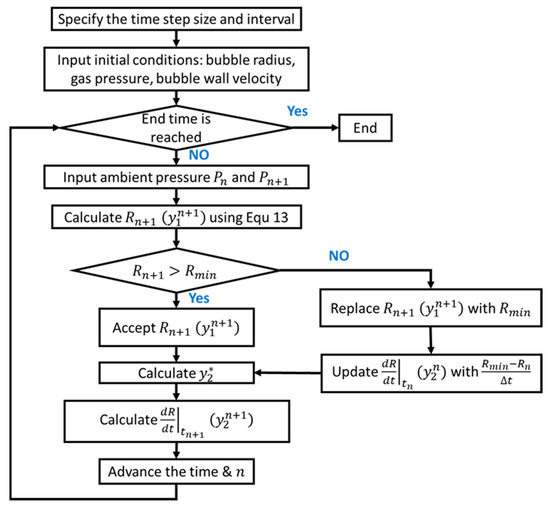
Figure 3.
Flowchart of Euler Algorithm.
Both the solution schemes presented here employ the truncation radius and accept a constant time step size. The solution schemes differ in three aspects: (i) the FD PC algorithm is a 1st order scheme while the Euler algorithm is a 2nd order scheme; (ii) the former algorithm only needs the ambient pressure of the current time step to be known, but the latter algorithm requires the ambient pressure of the next time step , which makes it unfriendly to the case where the ambient pressure profile transiently interplays with the vapor phase and is not known throughout; (iii) the former one takes into account the viscous effect in the collapse stage and the latter one includes the viscous effect all over the bubble development.
3. Validation
In order to verify the validity of the proposed solution schemes, calculated results are compared with published results from other researchers. The bubble radius evolutions obtained from the proposed solution schemes and published work are benchmarked for three types of ambient pressure paths: constant pressure, pressure in the Venturi tube, and sinusoidal oscillating pressure. These types of ambient pressure paths are selected because they are common in the hydrodynamic and ultrasonic cavitation studies.
3.1. Bubbles under Constant Pressure
It is well known that the analytical solution of the RP equation is readily obtainable for a simplified RP equation, where viscous and surface tension terms of RP are neglected [24]. The analytical solution is well established when the ambient pressure is constant and the viscous term is neglected. The analytical solution takes the form of Equation (19) if the isothermal condition is assumed. Depending on the initial state of bubbles and magnitude of the constant ambient pressure, response of the bubble radius to the ambient pressure can be categorized as oscillation and unlimited growth. The category is dictated by the roots of , where in Equation (20) is equivalent to the right side of (19). Apart from , which automatically satisfies , there may be one root or no root present. The former case corresponds to the oscillation type and the latter case corresponds to the unlimited growth. Details of bubble radius under constant pressure can be found in [25].
Although the above analytical solution implies that the viscous term is neglected, it is still a good standard to judge if the proposed solution schemes work. The validity of the proposed solution schemes will be evaluated in a more general case in the next sections. Table 1 shows the parameters used for benchmarking.

Table 1.
Input Variables.
Input variables listed in Table 1 leads to two roots of , which are labeled as and , respectively, in Figure 4. The root of 73 µm is located on the right side of root of 10 µm. Based on the theory above, this indicates that the bubble radius will oscillate between 10 µm and 73 µm. Evolution of the bubble radius acquired from the analytical solution is shown in Figure 5. Note: See Appendix A to reproduce Figure 5.
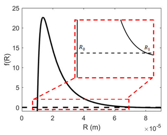
Figure 4.
Roots of .
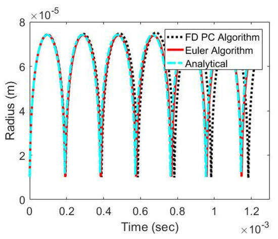
Figure 5.
Bubble Radius under Constant Pressure.
The analytical solution and two proposed solution schemes yield similar bubble radius evolutions. The bubble oscillates between and and a steep change of bubble radius is observed when the bubble approaches its minimum size. As shown in Figure 5, three methods give an almost identical bubble radius in the first two cycles of oscillation and a slight difference is observed as the time advances to more cycles. In the last cycle, it is observed that the Euler algorithm agrees with the analytical solution a little better than the FD PC algorithm. Nevertheless, the two proposed solution schemes are validated in this special case.
3.2. Bubbles under Pressure Emanating from a Venturi Tube
So far, the proposed solution schemes have shown to perform well in a special case where the viscous term is neglected and the ambient pressure is constant. The proposed schemes are further tested for a general case where the viscous term is preserved and the pressure is time varying. The Venturi tube is widely used to generate hydrodynamic cavitation. It forces the liquid through a constriction and the pressure drop caused by acceleration of liquid leads to the cavitation. Aleihossein et al. [23] presented a typical pressure history (Figure 6) which a bubble undergoes as it travels through the Venturi tube. They also predicted the bubble radius evolution using their own modified Euler and Runge–Kutta–Fehlberg solver with the pressure history shown in Figure 6 and parameters listed in Table 2.
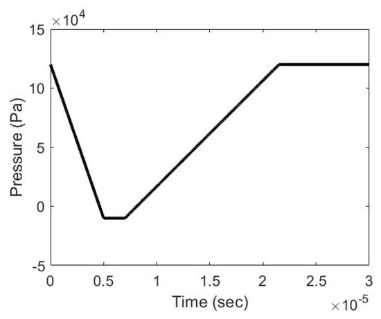
Figure 6.
Pressure Profile under Venturi.
Table 2.
Input Variables.
Using the pressure profile for the Venturi tube given in Figure 6 and parameters in Table 2, results of two proposed solution schemes and Alehossein’s method were benchmarked. As shown in Figure 7, all of them indicate that the bubble rapidly grows at the beginning and then collapses to a near-zero volume followed by a few cycles of rebounding. Since the liquid viscosity dissipates the kinetic energy of the bubble, rebounding is gradually dampened. The FD PC algorithm and Euler algorithm yield almost the same bubble evolution. It is clear that two proposed solution schemes slightly overestimate the bubble size compared to Alehossein’s method. For example, the maximum bubble radius given by the proposed approaches and Alehossein’s method is 36 µm and 28 µm, respectively. This overestimation also leads to a delay in bubble collapse and subsequent rebounding. Note: See Appendix A to reproduce Figure 7.
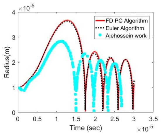
Figure 7.
Bubble Radius under Venturi Tube.
3.3. Bubbles under Sinusoidal Pressure Wave
Although results of the two proposed schemes slightly differ from Alehossein’s work on evolution of the bubble radius through the Venturi, it is safe to say that this difference is within the tolerances for most engineering applications. Therefore, the two proposed solution schemes are considered viable in typical scenarios of hydrodynamic cavitation. The ultrasonic cavitation is the other type of cavitation, where a fluctuating pressure field propagating in the liquid is responsible for the cavitation. In this type, the bubble experiences a sinusoidal-shaped pressure history. Hilgenfeldt et al. [26] calculated the bubble radius under a sinusoidal pressure shown in Figure 8. Other parameters they used are listed in Table 3.
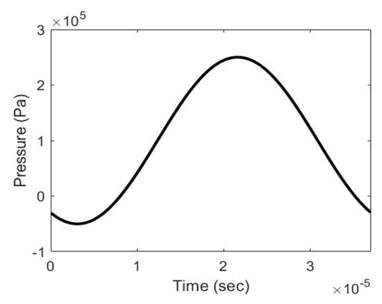
Figure 8.
Sinusoidal Pressure Wave.
Table 3.
Input Variables.
Results from the two proposed schemes and Hilgenfeldt’s work are benchmarked with the same input variables. As shown in Figure 9, all results indicate that the bubble growth is followed by a sequence of collapse and rebounding. Two proposed schemes slightly overestimate the bubble growth and show a delayed bubble collapse. Hilgenfeldt’s results showed that rebounding is gradually dampened and finally vanishes. Their results also showed that the bubble radius recovered when the ambient pressure declined at 20 µs. The Euler algorithm exhibits similar patterns of bubble radius, as shown in Figure 9. In contrast, the FD PC algorithm predicts a recovery of the bubble radius at the end, but rebounding does not show any sign of fading out (Figure 9). Undamped rebounding given by the FD PC algorithm may be because correction of the bubble wall velocity by the viscous effect is only carried out when the bubble size exceeds the threshold. Note: See Appendix A to reproduce Figure 9.
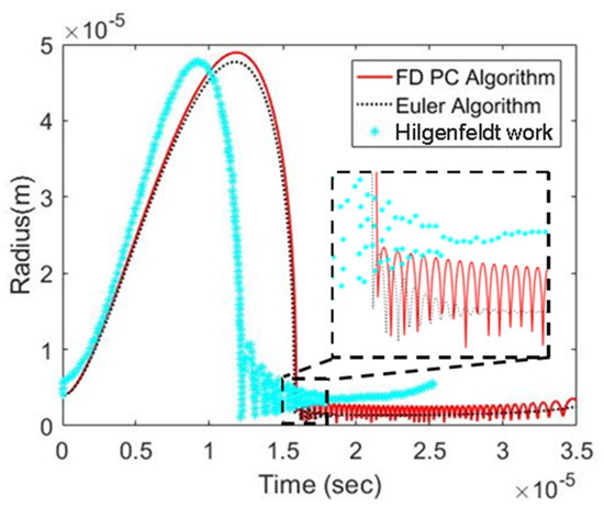
Figure 9.
Bubble Radius under Sinusoidal Pressure Wave.
4. Robustness
The previous section showed that two proposed solvers can give a fair prediction of bubble radius in the general cases of hydrodynamic and ultrasonic cavitation. Its accuracy should be able to satisfy requirements of most analyses in engineering. It was reported that the stiffness issue caused by a large pressure variation limits the capacity of the RP equation solver and reduces its efficiency [22,23,26]. Since two proposed schemes make an approximation of the bubble radius and wall velocity at the final stage of the bubble collapse using a truncation radius ( in Figure 2), it can overcome that singularity point with a relatively coarse time step.
A large pressure variation can be observed in the pressure pulsation created by the hydraulic machinery, such as the pump and valve. In order to test if the proposed scheme performs well in the case of a large pressure variation, an ambient pressure which mimics the pressure pulsation created by opening and closing of a valve is used. As shown in Equation (21), this ambient pressure is parametrized by w, A, B, which affect the period, amplitude, and location of the midline, respectively. Two parametric analyses (Analysis A and B) are carried out to study effects of A and B on the robustness of the proposed schemes. Values for parameters A and B are listed in Table 4. In addition to two proposed solution schemes, a commercial Matlab, ODE15s is used in Analysis A and B. ODE15s of Matlab is a variable-step, variable-order (VSVO) solver based on numerical differentiation formulas (NDFs) of orders 1 to 5. The results from this solver are used as the baseline.
Table 4.
Parameters: w, A, and B.
The ambient pressure used in Analysis A is shown in Figure 10 With A increasing from to , four ambient pressure curves with different variations are created and labeled as Tests 1–4 respectively. When parameter A is less or equal to , ODE15s and the two proposed schemes present similar bubble radius evolution as shown in Figure 11a–c. The Euler algorithm agrees with ODEs15s in terms of the bubble radius being better than in the FD PC algorithm. There was no substantial difference in the computational time between the proposed schemes and ODE15s. The solutions were completed within 6 s using a Dell computer (with 16 cores of Intel Xeon Processor E5-2630 v3@2.4 GHz and RAM of 128 GB). When a parameter A of was used, ODE15s stopped working because the variable time step size became much smaller than the built-in lower limit of s. In contrast, the two proposed algorithms were able to predict the bubble radius as shown in Figure 11d.
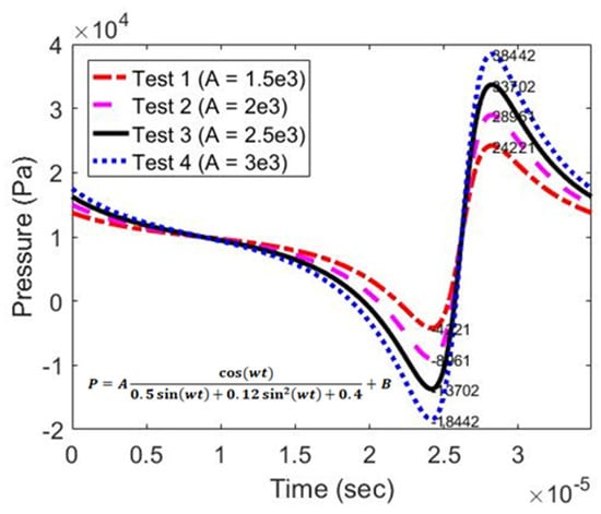
Figure 10.
Ambient Pressure profiles for testing the solution schemes (Tests 1–4).
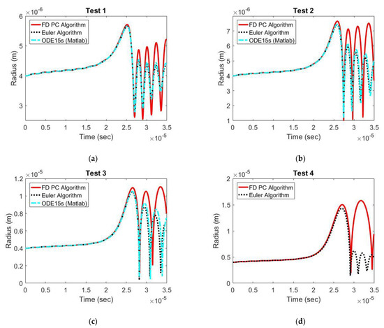
Figure 11.
Bubble radius for various ambient pressure profiles (Tests 1–4). (a) Test 1 , (b) Test 2 , (c) Test 3 , (d) Test 1 .
The performance of ODE15s and two proposed solution schemes is also benchmarked under different values of parameter B. In Analysis B, four ambient pressure curves shown in Figure 12 corresponding to values of B from to were used. As shown in Figure 13, apart from the case of , ODE15s and two proposed solution schemes yielded similar results of the bubble radius. In the case of , only two proposed solution schemes were able to solve the RP equation, as seen in Figure 13a.
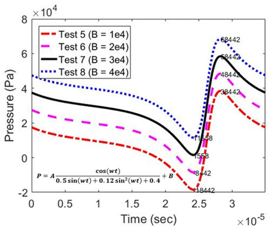
Figure 12.
Ambient pressure profiles for testing the solution schemes (Tests 5–8).
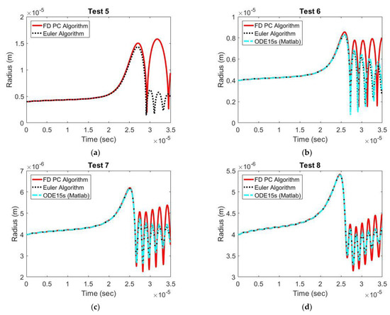
Figure 13.
Bubble Radius for various ambient pressure profiles (Tests 5–8). (a) Test 5 , (b) Test 6 , (c) Test 7 , (d) Test 8 .
In summary, variation in the ambient pressure profiles, which predetermines cavitation in fluid flows, can significantly affect the stiffness of the RP equation and functionality of the solver. The proposed solution schemes have shown to exhibit superiority in managing a wide range of ambient pressure compared to the general ODE solver available in Matlab.
5. Convergence
The truncation error in the finite difference method depends on the discretization size. As the discretization size approaches zero, a legitimate finite difference scheme should give results which converge and finally are consistent with the true solution of the equation. Convergence of the two proposed solution schemes is evaluated by varying the time step size from to s. The ambient pressure used in this case is Test 4 discussed in Section 4. As shown in Figure 14, regardless of the time step size, curves of the bubble radius coincide before the first collapse but differ in the rebounding phase. However, as the time step is refined below s, the rebounding phase starts to converge in the case of the FD PC algorithm. Similarly, the convergence of the Euler algorithm occurs at the time step size of s (Figure 15).
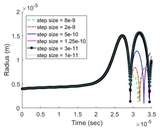
Figure 14.
Bubble Radius under Time Step Size of , , , , , and s (FD PC Algorithm).
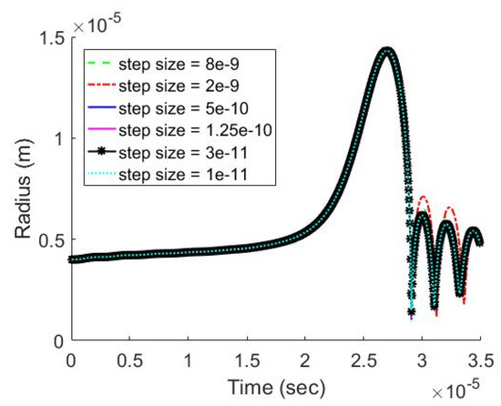
Figure 15.
Bubble Radius under Time Step Size of , , , , , and s (Euler Algorithm).
The convergence rate and computational efficiency of the two proposed schemes are compared. The error is defined in Equation (22), where is the approximate bubble radius and is the real bubble radius. It is assumed that the error is zero at the finest time step of s. As shown in Table 5, the Euler algorithm has a higher convergence rate than the FD PC algorithm. In contrast, the FD PC algorithm exhibits superior computational efficiency to the Euler algorithm.
n is the number of time steps.
Table 5.
Accuracy and Computational Efficiency of two Proposed Solution Schemes.
6. Conclusions
This study showed that the stiffness issue of the full form of the Rayleigh–Plesset (RP) equation caused by the steep variation in ambient pressure can be addressed by approximating the minimum bubble radius with a truncation value. By preserving the nonlinear terms, such as the viscous and acceleration terms, the proposed schemes can predict the bubble response more accurately than the reduced form of the RP equation. The proposed schemes are shown to be more robust than the traditional schemes using the variable time step when a wide range of ambient pressure is required. Thanks to the truncation bubble radius, the schemes avoid the excessive refinement of time step size at the singularity point, which is in favor of computational efficiency and its compatibility with CFD programs. Two solution schemes are presented: the finite difference-based prediction–correction scheme and the Euler method-based scheme. The first one partitions the RP equation such that one term of the RP equation is used as a correction term in the algorithm. The second one employs the 2nd-order Euler method. Compared to the first one, it is more accurate, converges faster, but consumes more computational time and requires the ambient pressure history to be known. For coupling the proposed solution schemes with CFD codes which solve the governing equations simultaneously, the FD PC algorithm will be more suitable than the Euler algorithm. It is demonstrated that both schemes yield similar results to the established ones in common scenarios of hydrodynamic and ultrasonic cavitation.
Author Contributions
Conceptualization and methodology, H.P.; formal analysis, validation, and original draft preparation H.P.; editing, supervision, project administration, and funding acquisition, G.N. All authors have read and agreed to the published version of the manuscript.
Funding
This research was funded by NSF-CMMI Award #2043325.
Data Availability Statement
No new data were created or analyzed in this study. Data sharing is not applicable to this article.
Acknowledgments
The authors would like to thank the National Science Foundation for its support.
Conflicts of Interest
The authors declare no conflict of interest.
Nomenclature
| Bubble radius | |
| Initial bubble radius | |
| Bubble radius at nth time step | |
| Radius threshold | |
| Minimum radius | |
| Vapor pressure | |
| Ambient pressure | |
| Initial gas pressure | |
| Ambient pressure at nth time step | |
| Time | |
| Time at nth time step | |
| Time step size | |
| Vapor volume fraction | |
| Vapor phase velocity | |
| Bubble wall velocity | |
| Bubble wall velocity at nth time step | |
| Prediction part of bubble wall velocity | |
| Prediction part of bubble wall velocity at nth time step | |
| Correction part of bubble wall velocity | |
| Correction part of bubble wall velocity at nth time step | |
| Vapor density | |
| Liquid density | |
| Kinematic viscosity | |
| Polytropic index | |
| Surface tension | |
| number of time step | |
| Mass transfer rate of vaporization | |
| Mass transfer rate of condensation |
Appendix A
In order to reproduce Figure 5, use parameters listed in Table 1. The minimum radius is in the range of 0.1~1 µm, which is 1/100~1/10 of the initial radius. The time step size is s.
References
- Melnichuk, M.; Gardavaud, Q.; Thiébaud, F.; Perreux, D. Temperature effect in cavitation risk assessments of polymers for hydrogen systems. Int. J. Hydrog. Energy 2020, 45, 23020–23026. [Google Scholar] [CrossRef]
- Ge, M.; Manikkam, P.; Ghossein, J.; Subramanian, R.K.; Coutier-Delgosha, O.; Zhang, G. Dynamic mode decomposition to classify cavitating flow regimes induced by thermodynamic effects. Energy 2022, 254, 124426. [Google Scholar] [CrossRef]
- Nor Saadah, M.Y.; Anandan, S.; Sivashanmugam, P.; Flores, E.M.M.; Ashokkumar, M. A correlation between cavitation bubble temperature, sonoluminescence and interfacial chemistry—A minireview. Ultrason. Sonochemistry 2022, 85, 105988. [Google Scholar]
- Ge, M.; Petkovšek, M.; Zhang, G.; Jacobs, D.; Coutier-Delgosha, O. Cavitation dynamics and thermodynamic effects at elevated temperatures in a small Venturi channel. Int. J. Heat Mass Transf. 2021, 170, 120970. [Google Scholar] [CrossRef]
- Zheng, Z.Y.; Wang, L.; Wei, T.Z.; Cai, W.H.; Li, H.; Yao, L.M.; Li, F.C. Experimental investigation of temperature effect on hydrodynamic characteristics of natural cavitation in rotational supercavitating evaporator for desalination. Renew. Energy 2021, 174, 278–292. [Google Scholar] [CrossRef]
- Ge, M.; Zhang, G.; Petkovšek, M.; Long, K.; Coutier-Delgosha, O. Intensity and regimes changing of hydrodynamic cavitation considering temperature effects. J. Clean. Prod. 2022, 338, 130470. [Google Scholar] [CrossRef]
- Ge, M.; Sun, C.; Zhang, G.; Coutier-Delgosha, O.; Fan, D. Combined suppression effects on hydrodynamic cavitation performance in Venturi-type reactor for process intensification. Ultrason. Sonochemistry 2022, 86, 106035. [Google Scholar] [CrossRef]
- Saleem, M.R.; Zia, S.; Ashraf, W.; Ali, I.; Qamar, S. The space–time CESE scheme for shallow water equations incorporating variable bottom topography and horizontal temperature gradients. Comput. Math. Appl. 2018, 75, 933–956. [Google Scholar] [CrossRef]
- Saleem, M.R.; Ali, I.; Qamar, S. Application of discontinuous Galerkin method for solving a compressible five-equation two-phase flow model. Results Phys. 2018, 8, 379–390. [Google Scholar] [CrossRef]
- Singhal, A.K.; Athavale, M.M.; Li, H.; Jiang, Y. Mathematical basis and validation of the full cavitation model. J. Fluids Eng. 2002, 124, 617–624. [Google Scholar] [CrossRef]
- Zwart, P.J.; Gerber, A.G.; Belamri, T. A two-phase flow model for predicting cavitation dynamics. In Proceedings of the Fifth International Conference on Multiphase Flow, Yokohama, Japan, 30 May–4 June 2004; Volume 152. [Google Scholar]
- Sauer, J.; Schnerr, G.H. Development of a new cavitation model based on bubble dynamics. J. Appl. Math. Mech. 2001, 81, 561–562. [Google Scholar] [CrossRef]
- Owis, F.M.; Nayfeh, A.H. Numerical simulation of 3-D incompressible, multi-phase flows over cavitating projectiles. Eur. J. Mech. B/Fluids 2004, 23, 339–351. [Google Scholar] [CrossRef]
- Bakir, F.; Rey, R.; Gerber, A.G.; Belamri, T.; Hutchinson, B. Numerical and experimental investigations of the cavitating behavior of an inducer. Int. J. Rotating Mach. 2004, 10, 15–25. [Google Scholar] [CrossRef]
- Deimel, C.; Günther, M.; Skoda, R. Application of a pressure based CFD code with mass transfer model based on the Rayleigh equation for the numerical simulation of the cavitating flow around a hydrofoil with circular leading edge. In EPJ Web of Conferences; EDP Sciences: Les Ulis, France, 2014; Volume 67, p. 02018. [Google Scholar]
- Bicer, B.; Sou, A. Bubble dynamics model for predicting the growth and collapse of cavitation bubbles in diesel injector. At. Sprays 2014, 24, 4712–4726. [Google Scholar] [CrossRef]
- Soliman, W.; Nakano, T.; Takada, N.; Sasaki, K. Modification of Rayleigh–Plesset theory for reproducing dynamics of cavitation bubbles in liquid-phase laser ablation. Jpn. J. Appl. Phys. 2010, 49, 116202. [Google Scholar] [CrossRef]
- Ye, Y.; Li, G. Modeling of hydrodynamic cavitating flows considering the bubble-bubble interaction. Int. J. Multiph. Flow 2016, 84, 155–164. [Google Scholar] [CrossRef]
- Ye, Y.; Zhu, X.; Lai, F.; Li, G. Application of the semi-analytical cavitation model to flows in a centrifugal pump. Int. Commun. Heat Mass Transf. 2017, 86, 92–100. [Google Scholar] [CrossRef]
- Žnidarčič, A.; Mettin, R.; Dular, M. Modeling cavitation in a rapidly changing pressure field–application to a small ultrasonic horn. Ultrason. Sonochem. 2015, 22, 482–492. [Google Scholar] [CrossRef]
- Lomakin, V.; Bibik, O. Numerical prediction of the gas content effect on the cavitation characteristics of the pump using the simplified Rayleigh-Plesset equation. In IOP Conference Series: Materials Science and Engineering; IOP Publishing: Bristol, UK, 2019; Volume 492, p. 012037. [Google Scholar]
- Shams, E.; Finn, J.; Apte, S.V. A numerical scheme for Euler–Lagrange simulation of bubbly flows in complex systems. Int. J. Numer. Methods Fluids 2011, 67, 1865–1898. [Google Scholar] [CrossRef]
- Alehossein, H.; Qin, Z. Numerical analysis of Rayleigh–Plesset equation for cavitating water jets. Int. J. Numer. Methods Eng. 2007, 72, 780–807. [Google Scholar] [CrossRef]
- Mancas, S.C.; Rosu, H.C. Evolution of spherical cavitation bubbles: Parametric and closed-form solutions. Phys. Fluids 2016, 28, 022009. [Google Scholar] [CrossRef]
- Franc, J.P.; Michel, J.M. Fundamentals of Cavitation; Springer: Berlin/Heidelberg, Germany, 2004. [Google Scholar]
- Hilgenfeldt, S.; Brenner, M.P.; Grossmann, S.; Lohse, D. Analysis of Rayleigh–Plesset Dynamics for Sonoluminescing Bubbles; Cambridge University Press: Cambridge, UK, 1998. [Google Scholar]
Disclaimer/Publisher’s Note: The statements, opinions and data contained in all publications are solely those of the individual author(s) and contributor(s) and not of MDPI and/or the editor(s). MDPI and/or the editor(s) disclaim responsibility for any injury to people or property resulting from any ideas, methods, instructions or products referred to in the content. |
© 2023 by the authors. Licensee MDPI, Basel, Switzerland. This article is an open access article distributed under the terms and conditions of the Creative Commons Attribution (CC BY) license (https://creativecommons.org/licenses/by/4.0/).