Fractional-Step Method with Interpolation for Solving a System of First-Order 2D Hyperbolic Delay Differential Equations

Abstract

In this article, we consider a delayed system of first-order hyperbolic differential equations. The presence of the delay term in first-order hyperbolic delay differential equations poses significant challenges in both analysis and numerical solutions. The delay term also makes it more difficult to use standard numerical methods for solving differential equations, as these methods often require that the differential equation be evaluated at the current time step. To overcome these challenges, specialized numerical methods and analytical techniques have been developed for solving first-order hyperbolic delay differential equations. We investigated and presented analytical results, such as the maximum principle and stability results. The propagation of discontinuities in the solution was also discussed, providing a framework for understanding its behavior. We presented a fractional-step method using a backward finite difference scheme and showed that the scheme is almost first-order convergent in space and time through the derivation of the error estimate. Additionally, we demonstrated an application of the proposed method to the problem of variable delay differential equations. We demonstrated the practical application of the proposed method to solving variable delay differential equations. The proposed algorithm is based on a numerical approximation method that utilizes a finite difference scheme to discretize the differential equation. We validated our theoretical results through numerical experiments.

1. Introduction

Modelling a variety of phenomena using delay partial differential equations (DPDEs) has drawn considerable attention in a number of fields, including those of biology, engineering control, and transportation scheduling [1,2]. The delay partial differential equation is a type of partial differential equation in which the solution depends not only on the current value of the unknown function, but also on its values at previous times. Therefore, the initial conditions must be specified over an initial segment or domain rather than just at a set of finite points. The domain in which the initial conditions are defined is called the initial set. If the delay argument is presented in the time variable, then the initial set segment is typically a time interval, and the initial conditions specify the value of the solution and its derivatives over this interval. The behavior of solutions of partial differential equations with delay can be complex and difficult to predict, even with simple initial conditions. In general, the solutions may exhibit oscillations or instability, which can be difficult to analyze mathematically. There are various numerical methods for solving partial differential equations with delay, including finite difference methods, finite element methods, and spectral methods. These methods can be used to approximate the solutions of partial differential equations with delay and analyze their behavior over time. However, these methods may require special treatment to handle the delay term in the equation. The theory of ordinary differential equations with delay terms is highly developed, but an analogous level of understanding does not exist for partial differential equations with time and space-dependent unknowns. While there have been several numerical methods proposed for solving these types of problems, the lack of a comprehensive theoretical framework hinders our ability to fully understand and optimize these methods. Bellen and Zennaro [3] provided a comprehensive introduction to the analysis and numerical computation of ordinary differential equations with delay terms, making it an ideal starting point for researchers and practitioners interested in this field. Their book covers the fundamental theory of delay differential equations, including stability analysis and numerical methods for their solutions. Due to delay terms, analytical solutions are difficult to obtain [4,5,6,7], whereas the numerical method can greatly compensate for the lack of analytical work. Stein [8] proposed a differential equation model that included stochastic effects owing to neuron stimulation. Afterwards, Stein expanded the work to include the postsynaptic potential amplitude distribution [9]. Stein transformed neuron variability into a numerical form in order to study the variability of neurons in a quantitative manner, by determining the characteristic function of the distribution and analyzing its mean and variance. The authors of ref. [10] proposed an explicit numerical scheme utilizing the finite difference method. This scheme can be applied when the delay and advance arguments are relatively small, and the authors employed Taylor series approximations to handle the difference arguments. In [11], the authors considered only point-wise delays of advection equations with shifts on the right side in space. The linear hyperbolic delay differential equations (DHDEs) in high dimensions have been studied by a limited number of researchers. An investigation of a hyperbolic delay partial differential equation was carried out by the author of [12,13,14,15]. They proved that the difference schemes were stable and consistent. The authors of [16] delved into a detailed discussion of the stability analysis of a hyperbolic equation with delay, which was formulated in a more general and encompassing manner. This work provided valuable insights into the stability properties of the equation, shedding light on its behavior in scenarios where delays come into play. The literature has addressed numerical treatments for hyperbolic partial differential equations and convergence analysis [17,18,19,20,21,22,23]. In the study of hyperbolic partial differential equations, maximum principles play a crucial role in analyzing the behavior of the solutions. The maximum principle is a powerful tool that provides a bound on the solution of a hyperbolic partial differential equation by comparing it to its initial and boundary conditions. Maximum principles for hyperbolic, parabolic, and elliptical differential equations(DE) were extensively studied in [24]. Existence results for hyperbolic systems of equations are concerned with showing that there exists a unique solution to the system under certain initial and boundary conditions. To prove the existence of solutions, one typically starts by defining a suitable function space for the solutions of the system. This function space should be equipped with a norm or metric that allows one to measure the size or regularity of the solutions. Once a function space has been defined, one can use various techniques to establish the existence of solutions. In some cases, one can use energy estimates and maximum principles to show that a solution exists and is unique. These methods involve using the physical properties of the system to derive inequalities that constrain the behavior of the solutions. A detailed description of the existence results for a hyperbolic system of equations was given by [25]. Peaceman and Rachford [26] first introduced the alternating direction implicit (ADI) method in 1955 as a numerical technique based on finite difference approximations. This property makes the ADI method a popular choice for solving a wide range of problems in computational science and engineering. Thomas et al. [27] described the alternating direction implicit (ADI) scheme as a cost-effective numerical technique for solving partial differential equations. They demonstrated the stability and accuracy of the ADI method, comparing it with other standard finite difference methods using analytical solutions for two problems that approximate different stages. The paper emphasized the computational advantages of the ADI method, particularly in terms of reducing the computational effort required to obtain accurate solutions for two-dimensional problems, which are often more challenging to solve than one-dimensional problems. Aderito et al. [28] utilized the alternating direction implicit (ADI) method for solving a two-dimensional hyperbolic partial differential equation (PDE), which encompasses both convection and diffusion phenomena. The authors approach provided an efficient and accurate solution to the hyperbolic PDE, making it useful for modeling various physical and engineering systems. Their work demonstrated the importance of applying efficient numerical methods to solving complex PDEs in order to obtain accurate and reliable solutions. In order to reduce the computational complexity, we applied the fractional-step method. The fractional-step method was extensively studied for two-dimensional parabolic equations [29,30,31].

This paper details the analysis of a fractional-step finite difference scheme for a system of hyperbolic delay partial differential equations. The scheme involves applying the upwind finite difference scheme to discretize the spatial derivatives of the 1D problems obtained after applying the scheme for the time derivative. The paper provides a proof of convergence of almost first-order in space and first-order in time for the proposed method. In addition, the work in this paper developed fractional-step methods for transient problems that are sufficiently general to include all previously introduced techniques. Finally, the general fractional-step difference equation was examined for consistency, stability, and convergence.

The article is organized as follows. The problem is considered in Section 2. The maximum principle and its consequences are presented in Section 3. In Section 4, we describe the fractional-step method. An error analysis is presented for the proposed methods in Section 5. Section 6 presents a differential equation with variable delay. The numerical illustration is presented in Section 7. The conclusions are presented in Section 8.

The norm for convergence analysis is $\parallel \mathit{\psi }\parallel =max\{\parallel {\psi }_1\parallel ,\parallel {\psi }_2\parallel ,\cdots ,\parallel {\psi }_r\parallel \}$, $\parallel {\psi }_k\parallel ={sup}_{(x,y,t)\in \overline{D}}\parallel {\psi }_k\parallel$.

2. Statement of Problem

The results of [8,10,12] motivate us to study the following problem. Find $\mathbf{u}=(u_1,u_2,\cdots ,u_r)$, $u_k\in C^{(1)}(D)$, $k=1,2,\cdots ,r$, such that

$$\begin{array}{cc}\hfill & {\mathfrak{L}}_k\mathbf{u}:=\frac{\partial u_k}{\partial t}+{\overline{a}}_k·\nabla u_k+\sum _{l=1}^r{c}_{kl}{u}_l(x-\delta ,y-\eta ,t)=f_k,(x,y,t)\in D,\hfill \end{array}$$

(1)

$$\begin{array}{cc}\hfill & u_k(x,y,t)={\varphi }_k(x,y,t),(x,y,t)\in ([-\delta ,0]\times [-\eta ,y_f]\cup [0,x_f]\times [-\eta ,0])\times [0,T],\hfill \end{array}$$

(2)

$$\begin{array}{cc}\hfill & u_k(x,y,0)=u_{k,0}(x,y),(x,y)\in [0,x_f]\times [0,y_f],k=1,2,\cdots ,r.\hfill \end{array}$$

(3)

The above equation, Equation (1), can be written as

$$\begin{array}{cc}\hfill & {\mathfrak{L}}_k\mathbf{u}:=\left\{\begin{array}{c}\frac{\partial u_k}{\partial t}+{\overline{a}}_k·\nabla u_k=f_k-\sum _{l=1}^r{c}_{kl}{\varphi }_l(x-\delta ,y-\eta ,t),\hfill \\ (x,y,t)\in ((0,\delta ]\times (0,y_f]\cup (0,x_f]\times (0,\eta ])\times (0,T],\hfill \\ \frac{\partial u_k}{\partial t}+{\overline{a}}_k·\nabla u_k=f_k-\sum _{l=1}^r{c}_{kl}{u}_l(x-\delta ,y-\eta ,t),\hfill \\ (x,y,t)\in (\delta ,x_f]\times (\eta ,y_f]\times (0,T],\hfill \end{array}\right.\hfill \end{array}$$

(4)

$$\begin{array}{cc}\hfill & u_k(x,y,0)=u_{k,0}(x,y),(x,y)\in [0,x_f]\times [0,y_f],\hfill \end{array}$$

(5)

where ${\overline{a}}_k=(a_{k1},a_{k2})$, $a_{kl}=a_{kl}(x,y)$, $\forall k,l$, $c_{kl}=c_{kl}(x,y)$, $k=1,2,\cdots ,r,$$l=1,2,\cdots ,r,$$a_{kl}>0,$$c_{kl}\le 0,$$D=(0,x_f]\times (0,y_f]\times (0,T]$. The functions $a_{kl},$$c_{kl},$$f_k$ are sufficiently differentiable on their domains where $\delta$ and $\eta$ are fixed positive constants. Further, it is assumed that $x_f=m_1\delta$ and $y_f=m_2\eta$ for some non-negative integers $m_1,m_2.$

3. Stability Analysis and Derivative Estimates

3.1. Maximum Principle

An adaptation of the barrier function technique is given in [32,33]. The maximum principle is also presented, and stability results are established.

Theorem 1.

[Maximum Principle] Let $\mathit{\psi }=({\psi }_1,{\psi }_2,\cdots ,{\psi }_r),{\psi }_i\in C(\overline{D})\cap C^{(1)}(D)$, $i=1,2,\cdots ,r$, be any function satisfying ${\mathfrak{L}}_k\mathit{\psi }\ge 0,(x,y,t)\in D,$${\psi }_k(x,y,0)\ge 0,(x,y)\in [0,x_f]\times [0,y_f]$. Then, ${\psi }_k(x,y,t)\ge 0,\forall (x,y,t)\in \overline{D}$, $k=1,2,\cdots ,r$.

Proof. 

Let $\mathit{s}=(s_1,\cdots ,s_r)$, $s_i(x,y,t)=1+x+y+t,$ and ${\mathfrak{L}}_k(\mathit{s})>0$. Further, let $\mu =max\left\{max\{-\frac{{\psi }_1}{s_1}\},max\{-\frac{{\psi }_2}{s_2}\},\cdots ,max\{-\frac{{\psi }_r}{s_r}\}\right\}$ and let $(x^{*},y^{*},t^{*})$ be the point at which $\mu =-\frac{{\psi }_k}{s_k}(x^{*},y^{*},t^{*})$. Then, $({\psi }_k+\mu s_k)(x^{*},y^{*},t^{*})=0$ and $({\psi }_k+\mu s_k)(x,y,t)\ge 0,\forall (x,y,t)\in \overline{D}.$ At the point $(x^{*},y^{*},t^{*})$, the function ${\psi }_k+\mu s_k$ attains its minimum, assuming the contradiction $\mu >0.$

Suppose $(x^{*},y^{*},t^{*})\in (0,\delta ]\times (0,y_f]\cup (0,x_f]\times (0,\eta ])\times (0,T]$, then

$$\begin{array}{cc}\hfill 0<{\mathfrak{L}}_k(\mathit{\psi }+\mu \mathit{s})& =\frac{\partial }{\partial t}({\psi }_k+\mu s_k)+a_{k1}\frac{\partial }{\partial x}({\psi }_k+\mu s_k)+a_{k2}\frac{\partial }{\partial y}({\psi }_k+\mu s_k)\le 0,\hfill \end{array}$$

i.e., it contradicts itself.

Suppose $(x^{*},y^{*},t^{*})\in (\delta ,x_f]\times (\eta ,y_f]\times (0,T],$ then

$$\begin{array}{cc}\hfill & 0<{\mathfrak{L}}_k(\mathit{\psi }+\mu \mathit{s})=\frac{\partial }{\partial t}({\psi }_k+\mu s_k)+a_{k1}\frac{\partial }{\partial x}({\psi }_k+\mu s_k)+a_{k2}\frac{\partial }{\partial y}({\psi }_k+\mu s_k)\hfill \\ & +\sum _{l=1}^r{c}_{kl}({\psi }_l+\mu s_l)(x^{*}-\delta ,y^{*}-\eta ,t)\le 0\hfill \end{array}$$

is a contradiction. This contradiction shows that $\mu \le 0.$ Therefore, ${\psi }_k(x,y,t)\ge 0,(x,y,t)\in \overline{D}.$ Hence, the proof is complete. □

Theorem 2.

[Stability Result] Let $\mathit{\psi }=({\psi }_1,{\psi }_2,\cdots ,{\psi }_r)$ be any function, then

$$\begin{array}{c}\hfill \parallel \mathit{\psi }(x,y)\parallel \le Cmax\{\underset{x,y}{max}\Vert \mathit{\psi }(x,y,0)\Vert ,\underset{(x,y,t)\in \overline{D}}{sup}|{\mathfrak{L}}_k\mathit{\psi }(x,y,t)|\},\forall (x,y,t)\in \overline{D},\end{array}$$

where C is a constant.

Proof. 

Let ${\mathit{\omega }}^{\pm }(x,y,t)=C{C}^{*}\mathit{s}(x,y,t)\pm \mathit{\psi }(x,y,t)$, where $C^{*}=max\{\underset{x,y}{max}\Vert \mathit{\psi }(x,y,0)\Vert ,\underset{k}{max}\{{sup}_{(x,y,t)\in D}\Vert {\mathfrak{L}}_k\mathit{\psi }(x,y,t)\Vert \}\}.$ Let ${\mathsf{\omega }}^{\pm }(x,y,0)\ge 0$ and ${\mathfrak{L}}_k{\mathsf{\omega }}^{\pm }(x,y,t)=C{C}^{*}{\mathfrak{L}}_k\mathit{s}\pm {\mathfrak{L}}_k\mathit{\psi }\ge 0.$ Then, by the above theorem, Theorem 1, we have

$$\begin{array}{c}\hfill |\mathit{\psi }(x,t)|\le Cmax\{\underset{x,y}{max}\Vert \mathit{\psi }(x,y,0)\Vert ,\underset{k}{max}\{\underset{(x,y,t)\in D}{sup}\Vert {\mathfrak{L}}_k\mathit{\psi }(x,y,t)\Vert \}\},\\ \hfill \forall (x,y,t)\in \overline{D}.\end{array}$$

□

Remark 1.

The solution to the problem, which continuously depends on the data, is called stable [34].

Remark 2.

As a consequence of the above stability result, one can conclude that, if it exists, the solution of the above problems, (4) and (5), is stable and unique.

3.2. Derivative Bounds

From the given differential equations, Equations (1)–(3), we can obtain the following bounds for the derivatives.

Lemma 1.

Let $\mathbf{u}$ represent the solution of system in (1)–(3). The derivatives of this function satisfy the following bounds $\left|\frac{{\partial }^i{u}_k}{\partial t^i}\right|\le C,$$0\le i\le 2$, $k=1,2,\cdots ,r.$

Proof. 

By integration over $[0,x]$, $x\in [0,x_f]$,

$$\begin{array}{c}\hfill \frac{\partial u_k}{\partial t}+{\overline{a}}_k·\nabla u_k+\sum _{l=1}^r{c}_{kl}{u}_l(x-\delta ,y-\eta ,t)=f_k,\end{array}$$

and by application of integration by parts we show that $\left|\frac{{\partial }^i{u}_k}{\partial t^i}\right|\le C$, and successive differentiation gives the desired results. □

3.3. Propagation of Discontinuities

Following the arguments of [3,15], the solution discontinuity propagation is presented. Let t be fixed, then

$$\begin{array}{cc}\hfill \underset{x\to {\delta }^{-}}{lim}{a}_{k1}{u}_{k,xx}& =f_{k,x}({\delta }^{-},y,t)-u_{k,xt}({\delta }^{-},y,t)-a_{k1,x}({\delta }^{-},y)u_{k,x}({\delta }^{-},y,t)\hfill \\ & -a_{k2,x}({\delta }^{-},y)u_{k,y}({\delta }^{-},y,t)-a_{k2}({\delta }^{-},y)u_{k,yx}({\delta }^{-},y,t)\hfill \\ & -\sum _{l=1}^r\left[c_{kl,x}({\delta }^{-},y)u_l(0^{-},y-\eta ,t)+c_{kl}({\delta }^{-},y)u_{l,x}(0^{-},y-\eta ,t)\right],\hfill \\ \hfill & =f_{k,x}({\delta }^{-},y,t)-u_{k,xt}({\delta }^{-},y,t)-a_{k1,x}({\delta }^{-},y)u_{k,x}({\delta }^{-},y,t)\hfill \\ & -a_{k2,x}({\delta }^{-},y)u_{k,y}({\delta }^{-},y,t)-a_{k2}({\delta }^{-},y)u_{k,yx}({\delta }^{-},y,t)\hfill \\ & -\sum _{l=1}^r\left[c_{kl,x}({\delta }^{-},y){\varphi }_l(0^{-},y-\eta ,t)+c_{kl}({\delta }^{-},y){\varphi }_{l,x}(0^{-},y-\eta ,t)\right],\hfill \end{array}$$

$$\begin{array}{cc}\hfill \underset{y\to {\eta }^{-}}{lim}{a}_{k2}{u}_{k,yy}& =f_{k,y}(x,{\eta }^{-},t)-u_{k,yt}(x,{\eta }^{-},t)-a_{k1}(x,{\eta }^{-})u_{k,xy}(x,{\eta }^{-},t)\hfill \\ & -a_{k1,y}(x,{\eta }^{-})u_{k,x}(x,{\eta }^{-},t)-a_{k2,y}(x,{\eta }^{-})u_{k,y}(x,{\eta }^{-},t)\hfill \\ & -\sum _{l=1}^r\left[c_{kl,y}(x,{\eta }^{-})u_l(x-\delta ,0^{-},t)+c_{kl}(x,{\eta }^{-})u_{l,y}(x-\delta ,0^{-},t)\right],\hfill \\ \hfill & =f_{k,y}(x,{\eta }^{-},t)-u_{k,yt}(x,{\eta }^{-},t)-a_{k1}(x,{\eta }^{-})u_{k,xy}(x,{\eta }^{-},t)\hfill \\ & -a_{k1,y}(x,{\eta }^{-})u_{k,y}(x,{\eta }^{-},t)-a_{k2,y}(x,{\eta }^{-})u_{k,y}(x,{\eta }^{-},t)\hfill \\ & -\sum _{l=1}^r\left[c_{kl,y}(x,{\eta }^{-}){\varphi }_l(x-\delta ,0^{-},t)+c_{kl}(x,{\eta }^{-},t){\varphi }_{l,y}(x-\delta ,0^{-},t)\right],\hfill \end{array}$$

and

$$\begin{array}{cc}\hfill \underset{x\to {\delta }^{+}}{lim}{a}_{k1}{u}_{k,xx}& =f_{k,x}({\delta }^{+},y,t)-u_{k,xt}({\delta }^{+},y,t)-a_{k1,x}({\delta }^{+},y)u_{k,x}({\delta }^{+},y,t)\hfill \\ & -a_{k2,x}({\delta }^{+},y)u_{k,y}({\delta }^{+},y,t)-a_{k2}({\delta }^{+},y)u_{k,yx}({\delta }^{+},y,t)\hfill \\ & -\sum _{l=1}^r\left[c_{kl,x}({\delta }^{+},y)u_l({\delta }^{+},y-\eta ,t)+c_{kl}({\delta }^{+},y)u_{l,x}({\delta }^{+},y-\eta ,t)\right],\hfill \\ \hfill & =f_{k,x}({\delta }^{+},y,t)-u_{k,xt}({\delta }^{+},y,t)-a_{k1,x}({\delta }^{+},y)u_{k,x}({\delta }^{+},y,t)\hfill \\ & -a_{k2,x}({\delta }^{+},y)u_{k,y}({\delta }^{+},y,t)-a_{k2}({\delta }^{+},y)u_{k,yx}({\delta }^{+},y,t)\hfill \\ & -\sum _{l=1}^r\left[c_{kl,x}({\delta }^{+},y)u_l(0^{+},y-\eta ,t)+c_{kl}({\delta }^{+},y)u_{l,x}(0^{+},y-\eta ,t)\right],\hfill \end{array}$$

$$\begin{array}{cc}\hfill \underset{y\to {\eta }^{+}}{lim}{a}_{k2}{u}_{k,yy}& =f_{k,y}(x,{\eta }^{+},t)-u_{k,yt}(x,{\eta }^{+},t)-a_{k1}(x,{\eta }^{+})u_{k,xy}(x,{\eta }^{+},t)\hfill \\ & -a_{k1,y}(x,{\eta }^{+})u_{k,x}(x,{\eta }^{+},t)-a_{k2,y}(x,{\eta }^{+})u_{k,y}(x,{\eta }^{+},t)\hfill \\ & -\sum _{l=1}^r\left[c_{kl,y}(x,{\eta }^{+})u_l(x-\delta ,{\eta }^{+},t)+c_{kl}(x,{\eta }^{+},t)u_{l,y}(x-\delta ,{\eta }^{+},t)\right],\hfill \\ \hfill & =f_{k,y}(x,{\eta }^{+},t)-u_{k,yt}(x,{\eta }^{+},t)-a_{k1}(x,{\eta }^{+})u_{k,xy}(x,{\eta }^{+},t)\hfill \\ & -a_{k1,y}(x,{\eta }^{+})u_{k,y}(x,{\eta }^{+},t)-a_{k2,y}(x,{\eta }^{+})u_{k,y}(x,{\eta }^{+},t)\hfill \\ & -\sum _{l=1}^r\left[c_{kl,y}(x,{\eta }^{+})u_l(x-\delta ,0^{+},t)+c_{kl}(x,{\eta }^{+},t)u_{l,y}(x-\delta ,0^{+},t)\right].\hfill \end{array}$$

It is observed that ${\varphi }_{l,x}(0^{-},y-\eta ,t)\ne u_{l,x}(0^{+},y-\eta ,t)$. Hence, $a_{k1}({\delta }^{+},y)u_{k,xx}({\delta }^{+},y,t)\ne a_{k1}({\delta }^{-},y)u_{k,xx}({\delta }^{-},y,t)$. Similarly, one can show that $a_{k2}(x,{\eta }^{+})u_{k,yy}(x,{\eta }^{+},t)\ne a_{k2}(x,{\eta }^{-})u_{k,yy}(x,{\eta }^{-},t)$ and multiples of $\delta$ and multiples of $\eta$ are primary discontinuity points [3].

4. The Fractional-Step Method

4.1. Temporal Discretization

Let the time domain be discretized as ${\overline{\mathsf{\Omega }}}_t^M=\{t_i|i=0,1,2,\cdots ,M\}$, where $t_i=t_0+i\Delta t$, $\Delta t=\frac{T}{M}$. Let us define the differential operators as follows:

$$\begin{array}{c}\hfill L_{k,x}\mathbf{u}:=a_{k1}\frac{\partial u_k}{\partial x}+\sum _{l=1}^r{\tilde{c}}_{kl}{u}_l(x-\delta ,y-\eta ,t),\\ \hfill L_{k,y}\mathbf{u}:=a_{k2}\frac{\partial u_k}{\partial y}+\sum _{l=1}^r{\check{c}}_{kl}{u}_l(x-\delta ,y-\eta ,t),\end{array}$$

where $c_{kl}={\tilde{c}}_{kl}+{\check{c}}_{kl}$. Then, the $k\mathrm{th}$ equation in (1) can be written as

$$\begin{array}{c}\hfill \frac{\partial u_k}{\partial t}+(L_{k,x}+L_{k,y})\mathbf{u}=f_k,k=1,2,\cdots ,r.\end{array}$$

Furthermore, to enable a more efficient computation, the source term is separated into two distinct components, $f_k={\tilde{f}}_k+{\check{f}}_k$. To discretize the problem in (1) in terms of the time variable, we adopt the following numerical scheme:

$$\begin{array}{cc}\hfill & \left\{\begin{array}{c}{\widehat{u}}_k^0=u_{k,0}(x,y),\hfill \\ (I_k+\Delta t{L}_{k,x}){\widehat{\mathbf{u}}}^{n+\frac{1}{2}}={\widehat{u}}_k^n+\Delta t{\tilde{f}}_k(t_{n+1}),\hfill \\ {\widehat{u}}_k^{n+\frac{1}{2}}(0,y)={\varphi }_k(0,y,t_{n+1}),\hfill \\ (I_k+\Delta t{L}_{k,y}){\widehat{\mathbf{u}}}^{n+1}={\widehat{u}}_k^{n+\frac{1}{2}}+\Delta t{\check{f}}_k(t_{n+1}),\hfill \\ {\widehat{u}}_k^{n+1}(x,0)={\varphi }_k(x,0,t_{n+1}),k=1,2,\cdots ,r,\hfill \end{array}\right.\hfill \end{array}$$

(6)

where ${\widehat{\mathbf{u}}}^n(x,y)$ is the exact solution of $\mathbf{u}$ at the time level $t=t_n$, the uniform step size is represented by $\Delta t$, and $I_k$ represents the identity operator. Using this method, we can approximate $u_k^n(x,y)$ to the solution $u_k(x,y,t)$ of (1) at the time levels $t_n=n\Delta t$, $n=0,1,\cdots ,M.$ The operators $(I_k+\Delta t{L}_{k,\nu })$ and $\nu =x,y$ satisfy the following maximum principles.

Similar to [30,35], we introduce the local error for the $k^{th}$ component, $e_{k,n+1}$, which is defined by

$$\begin{array}{c}\hfill e_{k,n+1}=u_k(t_{n+1})-{\overline{u}}_k^{n+1},\end{array}$$

where $u_k(t_n)=u_k(x,y,t_n)$ and ${\overline{u}}_k^{n+1}$, for $n=0,1,\cdots ,M-1$, are the solutions to the following problem:

$$\begin{array}{cc}\hfill & \left\{\begin{array}{c}{\overline{u}}_k^0=u_{k,0}(x,y),\hfill \\ (I_k+\Delta t{L}_{k,x}){\overline{\mathbf{u}}}^{n+\frac{1}{2}}=u_k^n+\Delta t{\tilde{f}}_k(t_{n+1}),\hfill \\ {\overline{u}}_k^{n+\frac{1}{2}}(0,y)={\varphi }_k(0,y,t_{n+1}),\hfill \\ (I_k+\Delta t{L}_{k,y}){\overline{\mathbf{u}}}^{n+1}={\overline{u}}_k^{n+\frac{1}{2}}+\Delta t{\check{f}}_k(t_{n+1}),\hfill \\ {\overline{u}}_k^{n+1}(x,0)={\varphi }_k(x,0,t_{n+1}).\hfill \end{array}\right.\hfill \end{array}$$

(7)

To optimize computational efficiency and minimize costs, we decomposed the original two-dimensional problem into two sets of one-dimensional problems.

Lemma 2.

Let $\mathit{\psi }$ be any function, if ${\psi }_1,{\psi }_2,\cdots ,{\psi }_r\in C^0(\overline{D})\cap C^1(D)$ satisfies $(I_k+\Delta t{L}_{k,x})\mathit{\psi }(x)$$\ge 0$, for $x\in D$, then ${\psi }_k(x)\ge 0$.

Proof. 

Let $\mathit{s}=(s_1,s_2,\cdots ,s_r)$, $s_i(x)=1+x$, and $(I_k+\Delta t{L}_{k,x})\mathit{s}>0$. Further, let $\mu =max\{max\{-\frac{{\psi }_1}{s_1}\},max\{-\frac{{\psi }_2}{s_2}\},\cdots ,max\{-\frac{{\psi }_r}{s_r}\}\{$ and let $x^{*}$ be the point at which $\mu =-\frac{{\psi }_k}{s_k}(x^{*})$. Then, $({\psi }_k+\mu s_k)(x^{*})=0$ and $({\psi }_k+\mu s_k)x\ge 0,\forall x\in \overline{D}.$ At the point $x^{*}$, the function ${\psi }_k+\mu s_k$ attains its minimum, assuming the contradiction $\mu >0.$ Suppose $x^{*}\in (0,\delta ],$ then

$$\begin{array}{cc}\hfill 0<(I_k+\Delta t{L}_{k,x})(\mathit{\psi }+\mu \mathit{s})(x^{*})& =({\psi }_k+\mu s_k)(x^{*})+\Delta t{a}_{k1}\frac{\partial }{\partial x}({\psi }_k+\mu s_k)(x^{*})\le 0,\hfill \end{array}$$

which is a contradiction. Similarly one can obtain the contradiction when $x^{*}\in (\delta ,x_f]$. Hence, the proof of the lemma is complete. □

Lemma 3.

[Local Truncation Error] Assume that $\left|\frac{{\partial }^i{u}_k}{\partial t^i}\right|\le C,$$(x,y,t)\in (0,x_f]\times (0,y_f]\times (0,T],$$0\le i\le 2$. Then, $\parallel e_{k,n}{\parallel }_{\infty }=C{(\Delta t)}^2$, where $u_k(t_n)={\overline{u}}^n(x,y)+{\overline{e}}_n$ and $u_k(t_n)=u_k(x,y,t_n)$, and the local truncation error of the scheme in (7) satisfies

$$\begin{array}{c}\hfill \parallel e_{k,n}{\parallel }_{\infty }=O{(\Delta t)}^2.\end{array}$$

(8)

Proof. 

The proof is similar to that of [30,35]. For that, one can express

$$\begin{array}{cc}\hfill u_k(t_{n-1})& =(I_k+\Delta t{L}_{k,x})\left[(I_k+\Delta t{L}_{k,y})u(t_n)-\Delta t{\check{f}}_k(x,y,t_n)\right]\hfill \\ & -\Delta t{\tilde{f}}_k(x,y,t_n)+O{(\Delta t)}^2,\hfill \\ \hfill u_k(t_{n-1})& =(I_k+\Delta t{L}_{k,x})\left[(I_k+\Delta t{L}_{k,y}){\overline{u}}_k(t_n)-\Delta t{\check{f}}_k(x,y,t_n)\right]-\Delta t{\tilde{f}}_k(x,y,t_n),\hfill \\ \hfill & (I_k+\Delta t{L}_{k,x})(I_k+\Delta t{L}_{k,y}){\overline{e}}_n=O{(\Delta t)}^2.\hfill \end{array}$$

Hence, by applying the maximum principle given in Theorem (1) for the operator $I_k+\Delta t{L}_{k,i}$, $i=x,y,$ we obtain the required result. □

Lemma 4.

[Global Truncation Error] If $Z_{k,i}$ and $z_k(x_i)$ are numerical exact solutions at the node $x=x_i$, then the global error, $E_{k,n}$, of the scheme in (6) satisfies the following:

$$\begin{array}{c}\hfill \underset{n\le T/\Delta t}{sup}{\parallel E_{k,n}\parallel }_{\infty }\le C\Delta t.\end{array}$$

Proof. 

We consider

$$\begin{array}{cc}\hfill & E_{k,n}=e_{k,n}+{\overline{u}}_k^n-{\widehat{u}}_k^n,\hfill \\ \hfill & (I_k+\Delta t{L}_{k,y})({\overline{u}}_k^n-{\widehat{u}}_k^n)={\overline{u}}_k^{(n-1+\frac{1}{2})}-{\widehat{u}}_k^{(n-1+\frac{1}{2})},\hfill \\ & (I_k+\Delta t{L}_{k,x})({\overline{u}}_k^{(n-1)+\frac{1}{2}}-{\widehat{u}}_k^{(n-1)+\frac{1}{2}})=E_{k,n-1},\hfill \\ \hfill & {\overline{u}}_k^n-{\widehat{u}}_k^n={(I_k+\Delta t{L}_{k,x})}^{-1}{(I_k+\Delta t{L}_{k,y})}^{-1}{E}_{k,n-1}.\hfill \end{array}$$

Making use of the arguments given in [30,35], we have $|E_{k,n}|\le C\Delta t$, which concludes the proof. □

Lemma 5.

Let ${\widehat{u}}_k^{n+\frac{1}{2}}$ and ${\widehat{u}}_k^{n+1}$ be the solutions defined by (6), then $|\frac{d^k{\widehat{u}}_k^{n+\frac{1}{2}}}{d{x}^k}|\le C$ and $|\frac{d^k{\widehat{u}}_k^{n+1}}{d{y}^k}|\le C$, for $k=0,1,2,3$, except at the primary discontinuity points.

Proof. 

From the differential equation given in (6) and the application of Lemma 2, one can obtain the desired derivative estimates. □

4.2. The Fully Discrete Scheme

We discretize the spatial domain as follows. Let N be the mesh points in both the x and y directions. Let us define the mesh lengths $\Delta x=\frac{x_f}{N},\Delta y=\frac{y_f}{N}$ and meshes ${\overline{\mathsf{\Omega }}}_x^N={\left\{x_i\right\}}_{i=0}^N$, ${\overline{\mathsf{\Omega }}}_y^N={\left\{y_i\right\}}_{i=0}^N$, $x_i=x_{i-1}+\Delta x$, $y_i=y_{i-1}+\Delta y$, and ${\widehat{u}}_k^0(x,y)=u_{k,0}(x,y)$. The backward finite difference operators are defined by $D_{k,x}^{-},D_{k,y}^{-}$: $D_{k,x}^{-}{\widehat{U}}_{k,i,y}^{n+\frac{1}{2}}={\displaystyle \frac{{\widehat{U}}_{k,i,y}^{n+\frac{1}{2}}-{\widehat{U}}_{k,i-1,y}^{n+\frac{1}{2}}}{\Delta x}}$, $D_{k,y}^{-}{\widehat{U}}_{k,x,j}^{n+1}={\displaystyle \frac{{\widehat{U}}_{k,x,j}^{n+1}-{\widehat{U}}_{k,x,j-1}^{n+1}}{\Delta y}},D_{k,t}^{+}={\displaystyle \frac{{\widehat{U}}_{k,i,y}^{n+\frac{1}{2}}-{\widehat{U}}_{k,i,y}^n}{\Delta t}}$, and the bilinear interpolation is defined by

$$\begin{array}{cc}\hfill I_{k,\delta }{\widehat{U}}_{k,i,y}^{n+\frac{1}{2}}& ={\widehat{U}}_{k,q,p}^{n+\frac{1}{2}}{l}_q(x_i-\delta )l_p(y_j-\eta )+{\widehat{U}}_{k,q+1,p}^{n+\frac{1}{2}}{l}_{q+1}(x_i-\delta )l_p(y_j-\eta ),\hfill \\ \hfill & +{\widehat{U}}_{k,q,p+1}^{n+\frac{1}{2}}{l}_q(x_i-\delta )l_{p+1}(y_j-\eta )+{\widehat{U}}_{k,q+1,p+1}^{n+\frac{1}{2}}{l}_{q+1}(x_i-\delta )l_{p+1}(y_j-\eta ),\hfill \\ \hfill I_{k,\eta }{\widehat{U}}_{k,x,j}^{n+1}& ={\widehat{U}}_{k,q,p}^{n+1}{l}_q(x_i-\delta )l_p(y_j-\eta )+{\widehat{U}}_{k,q+1,p}^{n+1}{l}_{q+1}(x_i-\delta )l_p(y_j-\eta ),\hfill \\ \hfill & +{\widehat{U}}_{k,q,p+1}^{n+1}{l}_q(x_i-\delta )l_{p+1}(y_j-\eta )+{\widehat{U}}_{k,q+1,p+1}^{n+1}{l}_{q+1}(x_i-\delta )l_{p+1}(y_j-\eta ),\hfill \end{array}$$

where $x_i-\delta \in (x_q,x_{q+1})$, $y_j-\eta \in (y_p,y_{p+1})$, $l_q(x)={\displaystyle \frac{x_{q+1}-x}{\Delta x}}$, $l_{q+1}(x)={\displaystyle \frac{x-x_q}{\Delta x}}$, $l_p(y)={\displaystyle \frac{y_{p+1}-y}{\Delta y}}$, and $l_{p+1}(y)={\displaystyle \frac{y-y_p}{\Delta y}}.$ Let $y=y_j$, then the first equation in (6) can be approximated as follows:

$$\begin{array}{c}\hfill {\displaystyle \frac{{\widehat{U}}_{k,i,y}^{n+\frac{1}{2}}-{\widehat{U}}_{k,i,y}^n}{\Delta t}}+a_{k1}(x_i,y){\displaystyle \frac{{\widehat{U}}_{k,i,y}^{n+\frac{1}{2}}-{\widehat{U}}_{k,i-1,y}^{n+\frac{1}{2}}}{\Delta x}}+\sum _{l=1}^r{\tilde{c}}_{kl}{I}_{\delta ,\eta }{\widehat{U}}_{l,i,y}^{n+\frac{1}{2}}={\tilde{f}}_k(x_i,y,t_{n+1}).\end{array}$$

(9)

Let $x=x_i$, then the second equation in (6) can be approximated as follows:

$$\begin{array}{c}\hfill {\displaystyle \frac{{\widehat{U}}_{k,x,j}^{n+1}-{\widehat{U}}_{k,x,j}^{n+\frac{1}{2}}}{\Delta t}}+a_{k2}(x,y_j){\displaystyle \frac{{\widehat{U}}_{k,x,j}^{n+1}-{\widehat{U}}_{k,x,j-1}^{n+1}}{\Delta y}}+\sum _{l=1}^r{\check{c}}_{kl}{I}_{\delta ,\eta }{\widehat{U}}_{l,x,j}^{n+1}={\check{f}}_k(x,y_j,t_{n+1}),\end{array}$$

(10)

$u_k(x,y,0)=u_{k,0}(x,y),(x,y)\in [0,x_f]\times [0,y_f].$

The difference scheme of (7) is as follows:

$$\begin{array}{c}\hfill \left\{\begin{array}{c}(I_k+\Delta t{L}_{k,x}^N){\overline{\mathbf{U}}}_{i,y}^{n+\frac{1}{2}}=u_k(x_i,y,t_n)+\Delta t{\tilde{f}}_k(x_i,y,t_{n+1}),\hfill \\ {\overline{U}}_{k,i,y}^{n+\frac{1}{2}}(0,y)={\varphi }_k(0,y,t_{n+1}),\hfill \\ (I_k+\Delta t{L}_{k,y}^N){\overline{\mathbf{U}}}_{x,j}^{n+1}={\overline{U}}_{k,x,j}^{n+\frac{1}{2}}+\Delta t{\check{f}}_k(x,y_j,t_{n+1}),\hfill \\ {\overline{U}}_{k,x,j}^{n+1}(x,0)={\varphi }_k(x,0,t_{n+1}),\hfill \end{array}\right.\end{array}$$

(11)

where $L_{k,x}^N=a_{k1}{D}_{k,x}^{-}+{\sum }_{l=1}^r{\tilde{c}}_{kl}{I}_{k,\delta }$ and $L_{k,y}^N=a_{k2}{D}_{k,y}^{-}+{\sum }_{l=1}^r{\check{c}}_{kl}{I}_{k,\eta }$, and

$$\begin{array}{c}\hfill \left\{\begin{array}{c}{\widehat{U}}_{k,i,j}^0=u_{k,0}(x_i,y_j),0\le i,j\le N,\hfill \\ (I_k+\Delta t{L}_{k,x}^N){\widehat{\mathbf{U}}}_{i,j}^{n+\frac{1}{2}}={\widehat{U}}_{k,i,j}^n+\Delta t{\tilde{f}}_k(x_i,y_j,t_{n+1}),\hfill \\ {\widehat{U}}_{k,i,j}^{n+\frac{1}{2}}(0,y)={\varphi }_k(0,y,t_{n+1}),\hfill \\ (I_k+\Delta t{L}_{k,y}^N){\widehat{\mathbf{U}}}_{i,j}^{n+1}={\widehat{U}}_{k,i,j}^{n+\frac{1}{2}}+\Delta t{\check{f}}_k(x_i,y_j,t_{n+1}),\hfill \\ {\widehat{U}}_{k,i,j}^{n+1}(x,0)={\varphi }_k(x,0,t_{n+1}),\hfill \end{array}\right.\end{array}$$

(12)

for $n=0,\cdots ,M-1$.

Note: from [36], it is easy to see that $|\psi (x_i-\delta ,y_j-\eta ,t_i)-I_{k,\delta }\psi (x_i,y_j,t_i)|\le C{N}^{-2}$.

4.3. Discrete Stability Results

Lemma 6.

[Discrete Maximum Principle ] Let ${\mathit{\psi }}_i$ be any mesh function such that $(I_k+\Delta t{L}_{k,x}^N){\mathit{\psi }}_i\ge 0$, $1\le i\le N,$${\mathit{\psi }}_0\ge 0$. Then, ${\mathit{\psi }}_i\ge 0,$$\forall i.$

Proof. 

Let $\mathit{s}=(s_1,s_2,\cdots ,s_r)$, $s_{k,i}=1+x_i$, $k=1,2,\cdots ,r$, then $(I_k+\Delta t{L}_{k,x}^N){\mathit{s}}_i>0$, $\forall i$, $s_{k,i}>0,\forall i$. Let $\kappa =max\left\{max\{-\frac{{\psi }_1}{s_1}\},max\{-\frac{{\psi }_2}{s_2}\},\cdots ,max\{-\frac{{\psi }_r}{s_r}\}\right\}$ and let $i^{*}$ be the point at which $-\frac{{\mathit{\psi }}_i^{*}}{{\mathit{s}}_i^{*}}$ attains its maximum. Then, ${\psi }_{k,i^{*}}+\kappa s_{k,i^{*}}=0$ for some k, and ${\psi }_{k,i^{*}}+\kappa s_{k,i^{*}}\ge 0,\forall i.$ Suppose that $\kappa >0$, then we arrive the contradictions that follow.

Let us assume that ${\chi }_{k,i}={\psi }_{k,i}+\kappa s_{k,i}.$ Let $1\le i^{*}\le \nu ,$ then

$$0<(I_k+\Delta t{L}_{k,x}^N){\mathsf{\chi }}_{i^{*}}={\chi }_{k,i^{*}}+\Delta t{a}_{k1}(x_{i^{*}},y_j)D_{k,x}^{-}{\chi }_{k,i^{*}}\le 0.$$

This is a contradiction. Similarly, for $\nu +1\le i^{*}\le N$, one can obtain the contradiction

$$\begin{array}{cc}\hfill 0<(I_k+\Delta t{L}_{k,x}^N){\mathsf{\chi }}_{i^{*}}& ={\chi }_{k,i^{*}}+\Delta t{a}_{k1}(x_{i^{*}},y_j)D_{k,x}^{-}{\chi }_{k,i^{*}}\hfill \\ & +\Delta t\sum _{l=1}^r{\tilde{c}}_{kl}(x_{i^{*}},y_j)I_{k,\delta }{\chi }_{k,i^{*}}\le 0.\hfill \end{array}$$

Hence the proof is complete. □

Lemma 7.

[Discrete Stability Result] Let ${\mathit{\psi }}_i$ be any mesh function, then $|{\mathit{\psi }}_i|\le Cmax\{$$max|(I_k+\Delta t{L}_{k,x}^N){\mathit{\psi }}_i|,$${max}_i|{\mathit{\psi }}_i|\}$, $\forall i$.

Note: similarly to the above lemmas, Lemmas 6 and 7, one can the prove discrete maximum principle and stability results for $(I_k+\Delta t{L}_{k,y}^N)$.

5. Error Analysis

There are $2r$ sets of differential equations in the semidiscrete problem in (6), the first r sets of equations have y as a parameter, and the next r sets of equations have x as parameter.

$$\begin{array}{c}\hfill \left\{\begin{array}{c}(I_k+\Delta t{L}_{k,x})\mathbf{z}(x)=u_k(x,y,t_n)+\Delta t{\tilde{f}}_k(x,y,t_{n+1}),0<x<x_f,\hfill \\ z_k(0)={\varphi }_k(0,y,t_{n+1}),\hfill \end{array}\right.\end{array}$$

(13)

where $z_k(x)={\overline{u}}_k^{n+\frac{1}{2}}(x,y)$ and the parameter is y.

Theorem 3.

For $1\le i\le N-1$, there exists a positive constant C, which is independent of $y,N$ such that

$$|z_k(x_i)-Z_{k,i}|\le C{N}^{-1},$$

where $\left\{Z_{k,i}\right\}$ is the numerical solution of (11) and $z_k(x)$ is the exact solution of (13).

Proof. 

The proof of the theorem can be defined similarly to the proof of Theorem 4.6 in [31], and using [37]. Consider the mesh function ${\mathsf{\Psi }}_{k,i}=C{N}^{-1}(1+x_i)\pm (z_k(x_i)-Z_{k,i}).$ This proves that $L_{k,x}^N{\overline{\mathsf{\Psi }}}_i\ge 0$ and ${\overline{\mathsf{\Psi }}}_{k,0}\ge \overline{0}$, hence we have the desired result. □

Similarly to the arguments in Equation (4.47) in [31], and from Theorem 3 and Lemma 5, we have the following:

$$\begin{array}{c}\hfill |z_k(x_i)-Z_{k,i}|\le C{N}^{-1}\Delta t,\mathrm{for}1\le i\le N-1.\end{array}$$

(14)

Since $z_k(x_i)={\overline{u}}_k^{n+\frac{1}{2}}(x_i,y)$ and $Z_{k,i}={\overline{U}}_{i,y}^{n+\frac{1}{2}}$, we can write (14) as

$$\begin{array}{c}\hfill |{\overline{u}}_k^{n+\frac{1}{2}}(x_i,y)-{\overline{U}}_{k,i,y}^{n+\frac{1}{2}}|\le C{N}^{-1}\Delta t,\mathrm{for}1\le i\le N-1.\end{array}$$

(15)

Now, ${\overline{U}}_{k,x,j}^{n+1}$ satisfies the following problem:

$$\begin{array}{c}\hfill \left\{\begin{array}{c}(I_k+\Delta t{L}_{k,y}^N){\overline{\mathbf{U}}}_{x,j}^{n+1}={\overline{U}}_{k,x,j}^{n+\frac{1}{2}}+\Delta t{\check{f}}_k(x,y_j,t_{n+1}),j=1,\cdots ,N-1,\hfill \\ {\overline{U}}_{k,x,0}^{n+1}={\varphi }_k(x,0,t_{n+1}).\hfill \end{array}\right.\end{array}$$

(16)

We used this theorem, Theorem 3, for finding the bound of $({\overline{u}}_k^{n+1}(x,y_j)-{\overline{U}}_{k,x,j}^{n+1})$. The following problem is considered:

$$\begin{array}{c}\hfill \left\{\begin{array}{c}(I_k+\Delta t{L}_{k,y}^N){\widehat{\mathbf{U}}}_{x,j}^{n+1}={\widehat{U}}_{k,x,j}^{n+\frac{1}{2}}+\Delta t{\check{f}}_k(x,y_j,t_{n+1}),j=1,\cdots ,N-1,\hfill \\ {\widehat{U}}_{k,x,0}^{n+1}={\varphi }_k(x,0,t_{n+1}).\hfill \end{array}\right.\end{array}$$

(17)

Now, let us take the same approach that we used in Theorem 3, then we have

$$\begin{array}{c}\hfill |{\overline{u}}_k^{n+1}(x,y_j)-{\widehat{U}}_{k,x,j}^{n+1}|\le C{N}^{-1}\Delta t,\mathrm{for}1\le j\le N-1,\end{array}$$

(18)

and from Theorem 1 in [38], we have

$$\begin{array}{c}\hfill \parallel {(I_k+\Delta t{L}_{k,y}^N)}^{-1}{\parallel }_{\infty }\le 1.\end{array}$$

(19)

In addition, from (16) and (17), we can deduce

$$\begin{array}{c}\hfill {\widehat{U}}_{k,x,j}^{n+1}-{\overline{U}}_{k,x,j}^{n+1}={(I_k+\Delta t{L}_{k,y}^N)}^{-1}({\widehat{U}}_{k,x,j}^{n+\frac{1}{2}}-{\overline{U}}_k^{n+\frac{1}{2}}(x,y_j)),\mathrm{for}1\le j\le N-1.\end{array}$$

(20)

Therefore, from (15), (18)–(20), and

$$\begin{array}{c}\hfill {\overline{u}}_k^{n+1}(x,y_j)-{\overline{U}}_{k,x,j}^{n+1}={\widehat{U}}_{k,x,j}^{n+1}-{\overline{U}}_{k,x,j}^{n+1}+{\overline{u}}_k^{n+1}(x,y_j)-{\widehat{U}}_{k,x,j}^{n+1},\end{array}$$

(21)

we obtain

$$\begin{array}{c}\hfill |{\overline{u}}_k^{n+1}(x,y_j)-{\overline{U}}_{k,x,j}^{n+1}|\le C{N}^{-1}\Delta t,\mathrm{for}1\le j\le N-1.\end{array}$$

(22)

Using the fully discrete scheme, we can now prove the convergence of (15) and (22).

Theorem 4.

Let $u_k$ be the $k^{th}$ component of the exact solution of (1), and let $U_k^n$ be its numerical solution at time $t=n\Delta t$. Then, there exists a positive constant C such that

$$\parallel u_k(x_i,y_j,t_n)-U_{k,i,j}^n{\parallel }_{\infty }\le C(N^{-1}+\Delta t),k=1,2,\cdots ,r,$$

for $1\le i,j\le N-1$.

Proof. 

The global error is as follows:

$$\begin{array}{c}\hfill \parallel u_k(x_i,y_j,t_n)-U_{k,i,j}^n\parallel \le \parallel u_k(x_i,y_j,t_n)-{\overline{u}}_{k,i,j}^n\parallel +\parallel {\overline{u}}_{k,i,j}^n-{\overline{U}}_{k,i,j}^n\parallel \\ \hfill +\parallel {\overline{U}}_{k,i,j}^n-U_{k,i,j}^n\parallel .\end{array}$$

(23)

Using Lemma 3, and by (15) and (22), we obtain

$$\begin{array}{c}\hfill \parallel u_k(x_i,y_j,t_n)-U_{k,i,j}^n\parallel \le C(N^{-1}+\Delta t)+\parallel {\overline{U}}_{k,i,j}^n-U_{k,i,j}^n\parallel .\end{array}$$

(24)

Now, from (11), we can write

$$\begin{array}{c}\hfill (I_k+\Delta t{L}_{k,x}^N)(I_k+\Delta t{L}_{k,y}^N){\overline{U}}_{k,i,j}^{n+1}=u_k(x_i,y_j,t_n)+\Delta t{\check{f}}_k(x_i,y_j,t_{n+1})+\Delta t(I_k\\ \hfill +\Delta t{L}_{k,x}){\tilde{f}}_k(x_i,y_j,t_n).\end{array}$$

(25)

From 12, we have

$$\begin{array}{c}\hfill (I_k+\Delta t{L}_{k,x}^N)(I_k+\Delta t{L}_{k,y}^N)U_{k,i,j}^{n+1}=U_{k,i,j}^n+\Delta t{\check{f}}_k(x_i,y_j,t_{n+1})\\ \hfill +\Delta t(I_k+\Delta t{L}_{k,x}){\tilde{f}}_k(x_i,y_j,t_n),\end{array}$$

(26)

and subtracting (26) from (25) and applying the inverse operators ${(I_k+\Delta t{L}_{k,x}^N)}^{-1}$ and ${(I_k+\Delta t{L}_{k,y}^N)}^{-1}$, we obtain

$$\begin{array}{c}\hfill {\overline{U}}_{k,i,j}^{n+1}-U_{k,i,j}^{n+1}={(I_k+\Delta t{L}_{k,x}^N)}^{-1}{(I_k+\Delta t{L}_{k,y}^N)}^{-1}(u_k(x_i,y_j,t_n)-U_{k,i,j}^n).\end{array}$$

(27)

We can conclude that

$$\begin{array}{c}\hfill \parallel {\overline{U}}_{k,i,j}^{n+1}-U_{k,i,j}^{n+1}{\parallel }_{\infty }\le {\parallel u_k(x_i,y_j,t_n)-U_{k,i,j}^n\parallel }_{\infty },\end{array}$$

(28)

since

$$\begin{array}{c}\hfill \parallel {(I_k+\Delta t{L}_{k,x}^N)}^{-1}{\parallel }_{\infty }\le 1\mathrm{and}{\parallel {(I_k+\Delta t{L}_{k,y}^N)}^{-1}\parallel }_{\infty }\le 1.\end{array}$$

(29)

In this case, we replace $\parallel {\overline{U}}_{k,i,j}^n-U_{k,i,j}^n{\parallel }_{\infty }$ in (24) given the bound in (28) and we obtain

$$\begin{array}{c}\hfill \parallel u_k(x_i,y_j,t_n)-U_{k,i,j}^n{\parallel }_{\infty }\le C(N^{-1}+\Delta t),\end{array}$$

(30)

for $1\le i,j\le N-1$. This is the desired result. □

6. The Variable Delay Problem

Motivated by the study of [39,40], we considered the following 2D hyperbolic variable delay differential equation:

$$\begin{array}{cc}\hfill & {\mathfrak{L}}_k\mathbf{u}:=\frac{\partial u_k}{\partial t}+\overline{a_k}·\nabla u_k+\sum _{l=1}^n{c}_{kl}{u}_l(x-\delta (x),y-\eta (y),t)=f_k,(x,y,t)\in D,\hfill \end{array}$$

(31)

$$\begin{array}{cc}\hfill & u_k(x,y,t)={\varphi }_k(x,y,t),(x,y,t)\in ([{\zeta }_1,0]\times [{\zeta }_2,y_f]\cup [0,x_f]\times [{\zeta }_2,0])\times [0,T],\hfill \end{array}$$

(32)

$$\begin{array}{cc}\hfill & u_k(x,y,0)=u_{k,0}(x,y),(x,y)\in [0,x_f]\times [0,y_f],k=1,2,\dots ,r.\hfill \end{array}$$

(33)

The functions $a_{kl},c_{kl},$ and $f_k$ satisfying the conditions defined in Section 2 and $x-\delta (x)\le 0$, $x-\eta (x)\le 0$. We also have that ${\zeta }_1=min\{{inf}_{x\in [0,x_f]}x-\delta (x),0\}$ and ${\zeta }_2=min\{{inf}_{y\in [0,y_f]}y-\eta (y),0\}$. By Theorem 2, the solution is stable. Let $y=y_j,$ then $L_{k,x}{u}_k(x_i,y)$ is approximated as follows:

$$\begin{array}{c}\hfill a_{k1}(x_i,y)D_x^{-}{U}_{k,i,y}^{n+\frac{1}{2}}+\sum _{l=1}^r{\tilde{c}}_{kl}{I}_{k,\delta }{U}_{l,i,y}^{n+\frac{1}{2}}={\tilde{f}}_k(x_i,y,t_{n+1}).\end{array}$$

(34)

Let $x=x_i$, then $L_{k,y}{u}_k(x,y_j)$ is approximated as follows:

$$\begin{array}{c}\hfill a_{k2}(x,y_j)D_y^{-}{U}_{k,x,j}^{n+1}+\sum _{l=1}^r{\check{c}}_{kl}{I}_{k,\eta }{U}_{l,x,j}^{n+1}={\check{f}}_k(x_i,y,t_{n+1}).\end{array}$$

(35)

Where $u_k(x,y,0)=u_{k,0}(x,y),(x,y)\in [0,x_f]\times [0,y_f]$ in (34) and (35). Section 7 contains a numerical example problem with variable delay arguments.

The Algorithm for Solving the Problem

A variable delay algorithm is as defined as follows.

• Define mesh points $t_{n+1}$, $x_i$, $y_j$ with step lengths $\Delta t$, $\Delta x$, $\Delta y$, respectively.
• Assume $U_k=u_{k,0}(x_i,y_j),$ for all $i,j.$
• Replace $U_k=V_k,k=1,2,\cdots ,r.$
• If $x(i)-\delta (x(i))\le 0$, then $U_{k,i+1,j}={\left(\frac{1}{\Delta t}+\frac{a_{k1}(x_i,y_j)}{\Delta x}\right)}^{-1}\times [{\tilde{f}}_k(x_i,y_j,t_{n+1})+\frac{V_{k,i+1,j}}{\Delta t}$$+{\displaystyle \frac{a_{k1}(x_i,y_j)U_{k,i,j}}{\Delta x}}-{\sum }_{l=1}^r{\tilde{c}}_{kl}{\varphi }_l(x_i-\delta (x_i),y_j-\eta (y_j),t_{n+1})$.
• If $x(q)\le x(i)-\delta (x(i))\le x(q+1)$ and $y(p)\le y(j)-\eta (y(j))\le y(p+1)$, then $U_{k,i+1,j}={\left(\frac{1}{\Delta t}+\frac{a_{k1}(x_i,y_j)}{\Delta x}\right)}^{-1}\times [{\tilde{f}}_k(x_i,y_j,t_{n+1})+\frac{V_{k,i+1,j}}{\Delta t}+{\displaystyle \frac{a_{k1}(x_i,y_j)U_{k,i,j}}{\Delta x}}-{\sum }_{l=1}^r{\tilde{c}}_{kl}[U_{k,q,p}{l}_q(x_i-\delta )l_p(y_j-\eta )+U_{k,q+1,p}{l}_{q+1}(x_i-\delta )l_p(y_j-\eta )+U_{k,q,p+1}{l}_q(x_i-\delta )l_{p+1}(y_j-\eta )+U_{k,q+1,p+1}{l}_{q+1}(x_i-\delta )l_{p+1}(y_j-\eta )]$.
• Replace $U_k=V_k,k=1,2,\cdots ,r.$
• If $y(j)-\eta (y(j))\le 0$, then $U_{k,i,j+1}={\left(\frac{1}{\Delta t}+\frac{a_{k2}(x_i,y_j)}{\Delta y}\right)}^{-1}\times [{\check{f}}_k(x_i,y_j,t_{n+1})+\frac{V_{k,i,j+1}}{\Delta t}$
  $+{\displaystyle \frac{a_{k2}(x_i,y_j)U_{k,i,j}}{\Delta y}}-{\sum }_{l=1}^r{\check{c}}_{kl}{\varphi }_l(x(i)-\delta (x(i)),y(j)-\eta (y(j)),t(n+1))]$.
• If $x(q)\le x(i)-\delta (x(i))\le x(q+1)$ and $y(p)\le y(j)-\eta (y(j))\le y(p+1)$, then $U_{k,i,j+1}={\left(\frac{1}{\Delta t}+\frac{a_{k2}(x_i,y_j)}{\Delta y}\right)}^{-1}\times [{\check{f}}_k(x_i,y_j,t_{n+1})+\frac{V_{k,i,j+1}}{\Delta t}+{\displaystyle \frac{a_{k2}(x_i,y_j)U_{k,i,j}}{\Delta y}}-{\sum }_{l=1}^r{\check{c}}_{kl}[U_{k,q,p}{l}_q(x_i-\delta )l_p(y_j-\eta )+U_{k,q+1,p}{l}_{q+1}(x_i-\delta )l_p(y_j-\eta )+U_{k,q,p+1}{l}_q(x_i-\delta )l_{p+1}(y_j-\eta )+U_{k,q+1,p+1}{l}_{q+1}(x_i-\delta )l_{p+1}(y_j-\eta )]$.
• Go to Step 3 with $t=t+\Delta t$.

7. Numerical Examples

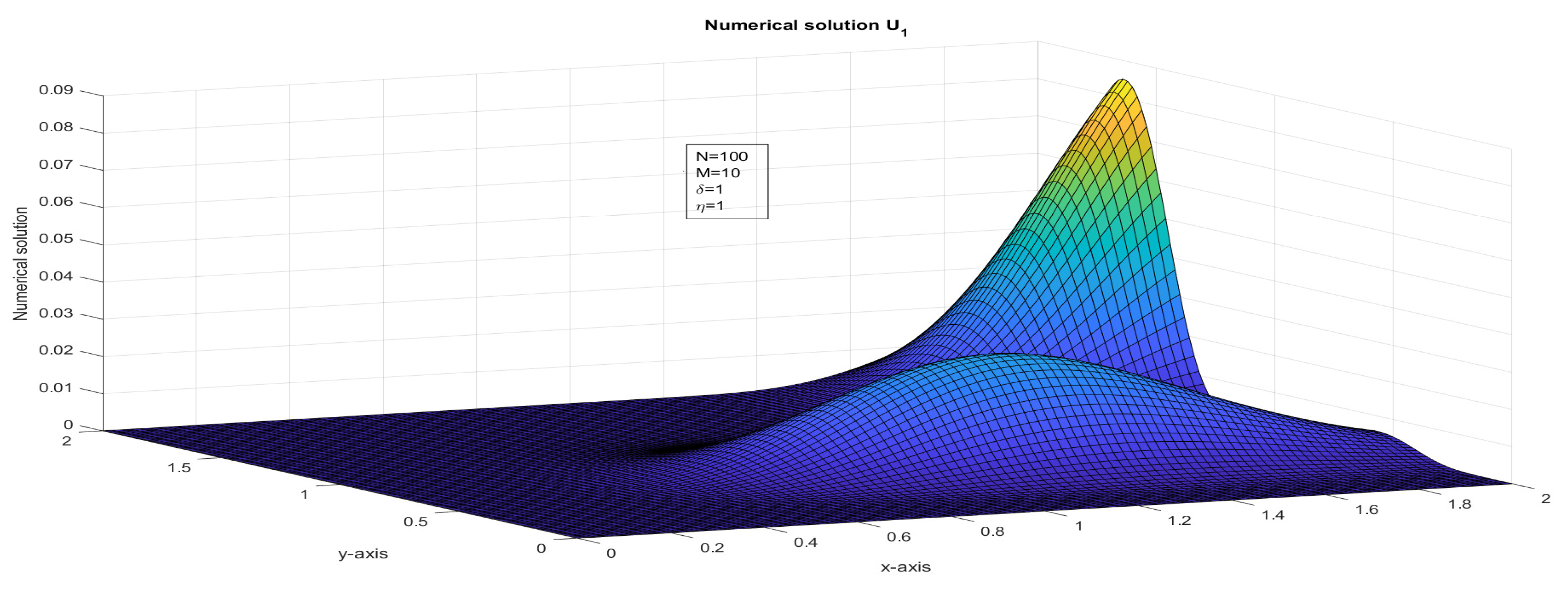
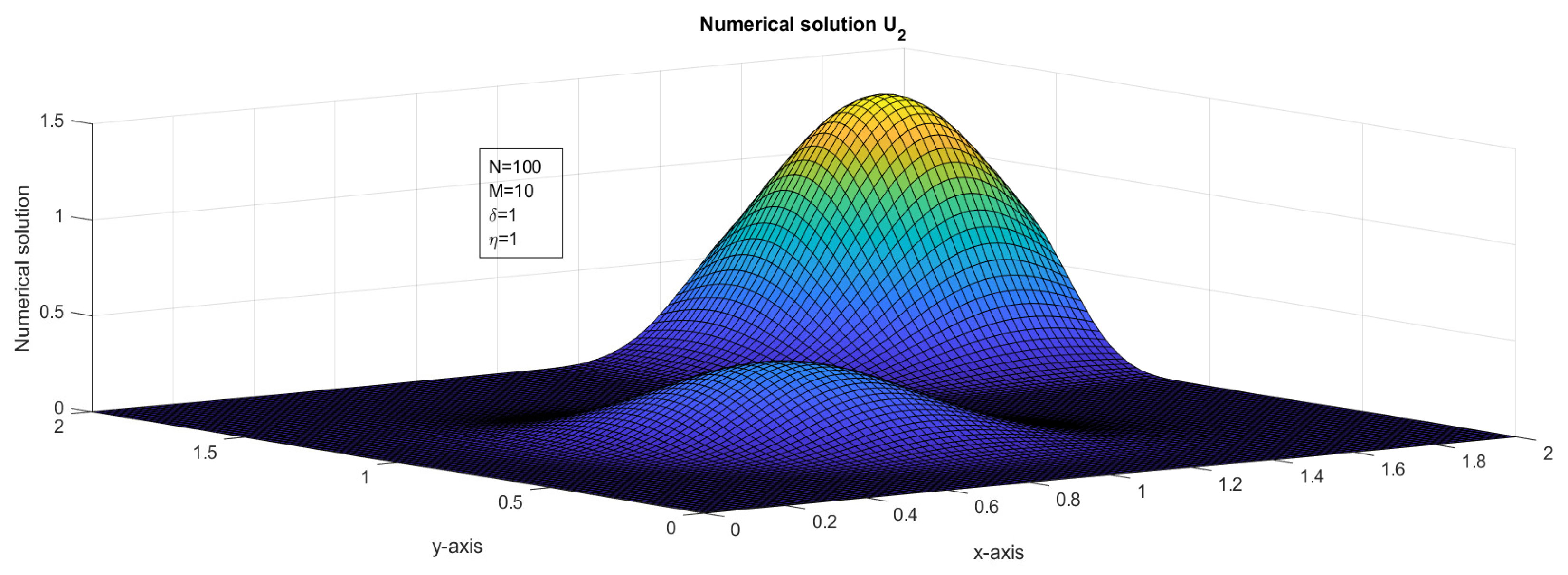
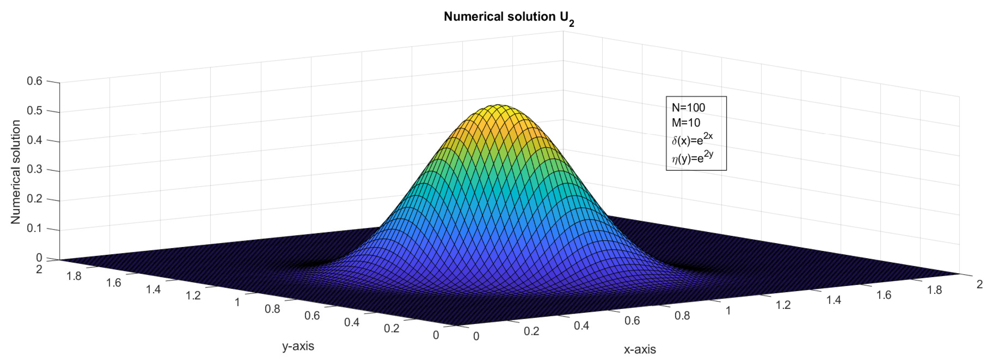
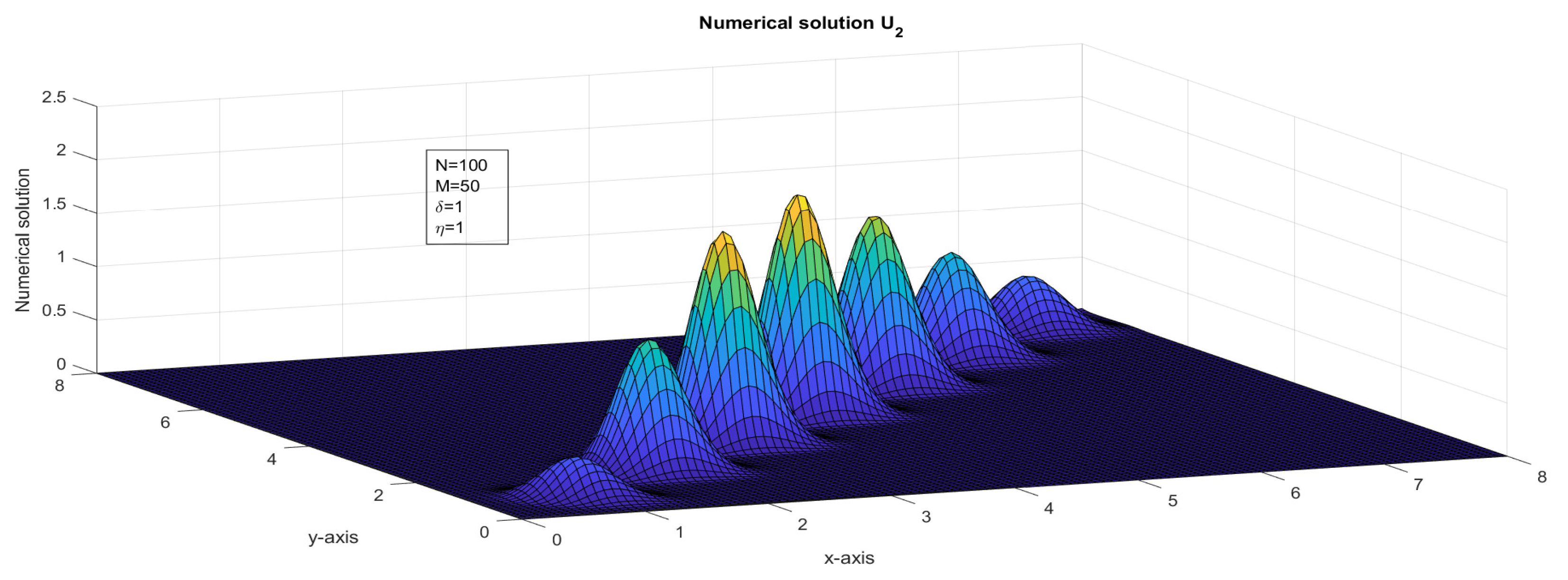
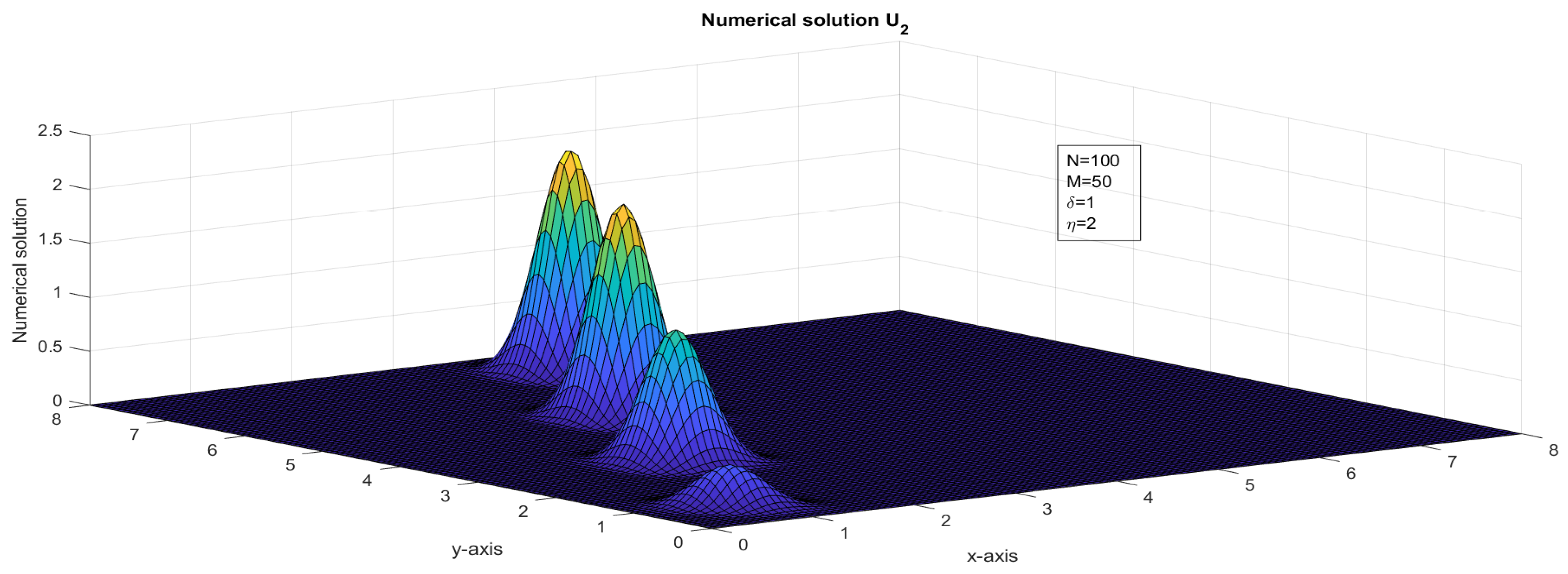
This section includes two examples that serve to confirm the validity of the theoretical results presented in the article. Figure 1, Figure 2, Figure 3, Figure 4, Figure 5, Figure 6, Figure 7, Figure 8, Figure 9, Figure 10, Figure 11, Figure 12, Figure 13, Figure 14, Figure 15 and Figure 16 display the plotted numerical solutions of the test problems, along with the corresponding maximum point-wise errors. To estimate the maximum error, we applied the half mesh principle stated in [31].

$$\begin{array}{cc}\hfill & E_k^{N,M}=\underset{i,j}{max}\mid U_{k,i,j}^M(\Delta x,\Delta y,\Delta t)-U_{k,i,j}^M(\Delta x/2,\Delta y/2,\Delta t/2)\mid ,0\le i,j\le N,\hfill \\ \hfill & D_{k,x,y}^N=\underset{M}{max}{E}_k^{N,M},D_{k,t}^M=\underset{N}{max}{E}_k^{N,M},\hfill \end{array}$$

where $U_{k,i,j}^M(\Delta x,\Delta y,\Delta t)$ and $U_{k,i,j}^M(\Delta x/2,\Delta y/2,\Delta t/2)$ are the numerical solutions at the node $(x_i,y_j,t_n)$, with mesh sizes $(\Delta x,\Delta y,\Delta t)$ and $(\frac{\Delta x}{2},\frac{\Delta y}{2},\frac{\Delta t}{2})$, respectively, and $D_{k,x,y}^N$ is the maximum over M for fixed N and $D_{k,t}^M$ is the maximum over N for fixed M. Numerical results and maximum point-wise errors were plotted.

Example 1.

Consider the following 2D hyperbolic DPDE with the following data.

$$\begin{array}{cc}\hfill & \frac{\partial u_k}{\partial t}+\overline{a_k}·\nabla u_k+\sum _{l=1}^2{c}_{kl}{u}_l(x-\delta ,y-\eta ,t)=f_k,\hfill \\ & (x,y,t)\in (0,2]\times (0,2]\times (0,1],k=1,2,\hfill \\ \hfill & u_k(x,y,t)=0,(x,y,t)\in ([-1,0]\times [-1,x_f]\cup [0,y_f]\times [-1,0])\times [0,T],\hfill \\ \hfill & u_1(x,y,0)=exp(-{(10x-1)}^5/4)\times exp(-{(4y-1)}^2/4)\times (2x-x^2)\times (2y-y^2),\hfill \\ \hfill & u_2(x,y,0)=exp(-{(6x-1)}^2/4)\times exp(-{(10y-1)}^5/4)\times (4x-x^2)\times (4y-y^2),\hfill \end{array}$$

$$\begin{array}{cc}\hfill & a_{11}={\displaystyle \frac{1+x^2+y^2}{1+2xy+x^2+y^2}},a_{12}={\displaystyle \frac{1+x^4+y^4}{1+2xy+2x^2+2y^2}},a_{21}={\displaystyle \frac{1+x^4+y^4}{1+2xy+3x^2+4y^2}},\hfill \\ & a_{22}={\displaystyle \frac{1+x^2+y^2}{1+2tx+3x^2+6y^2}},c_{11}=-1,c_{12}=-\frac{1}{2},c_{21}=-1,c_{22}=-\frac{1}{2},\hfill \\ & f_1=0=f_2.\hfill \end{array}$$

Case 1:

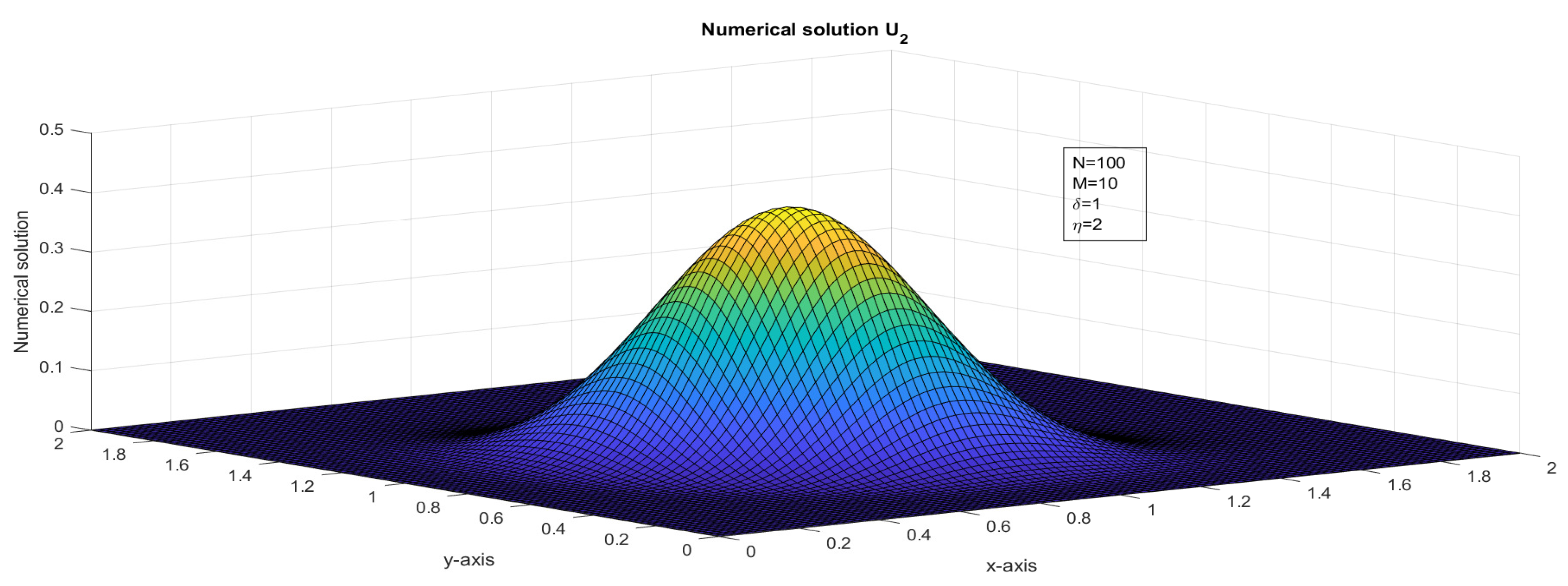
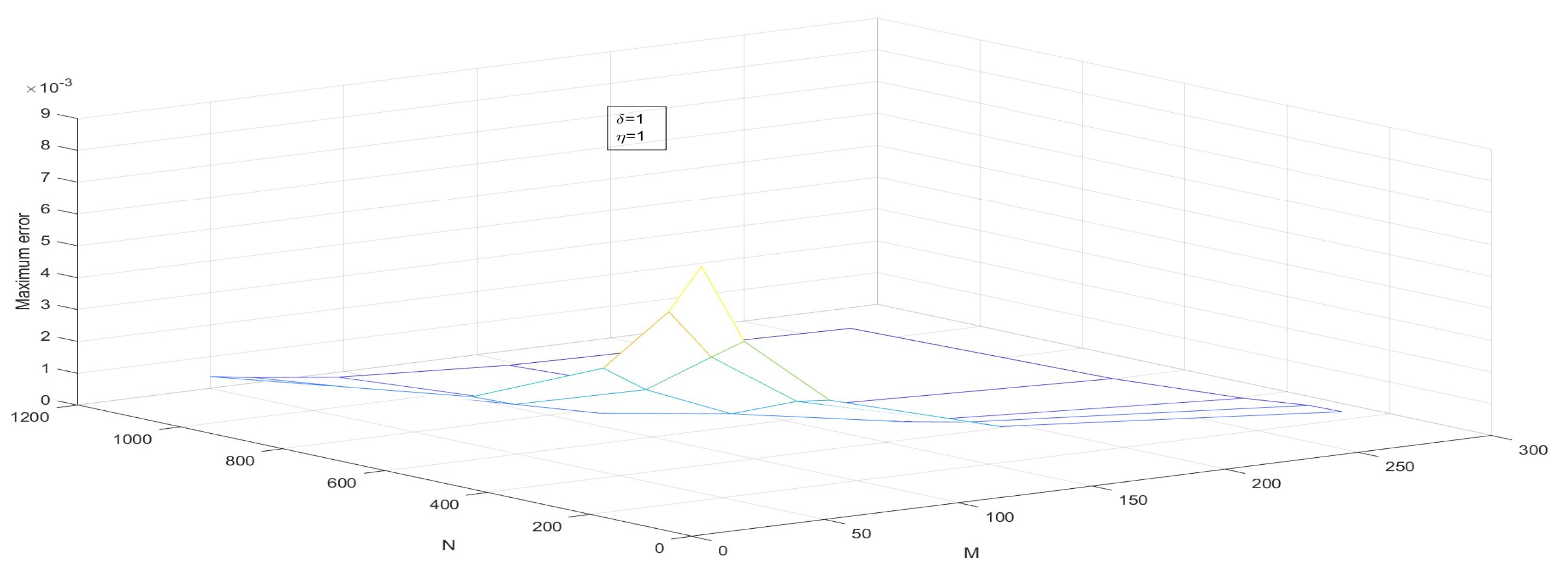
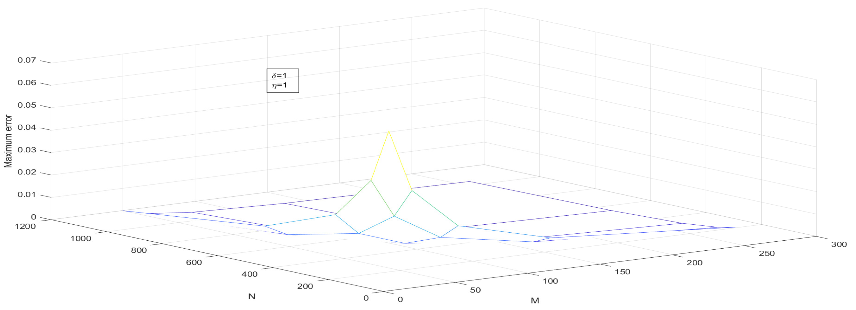
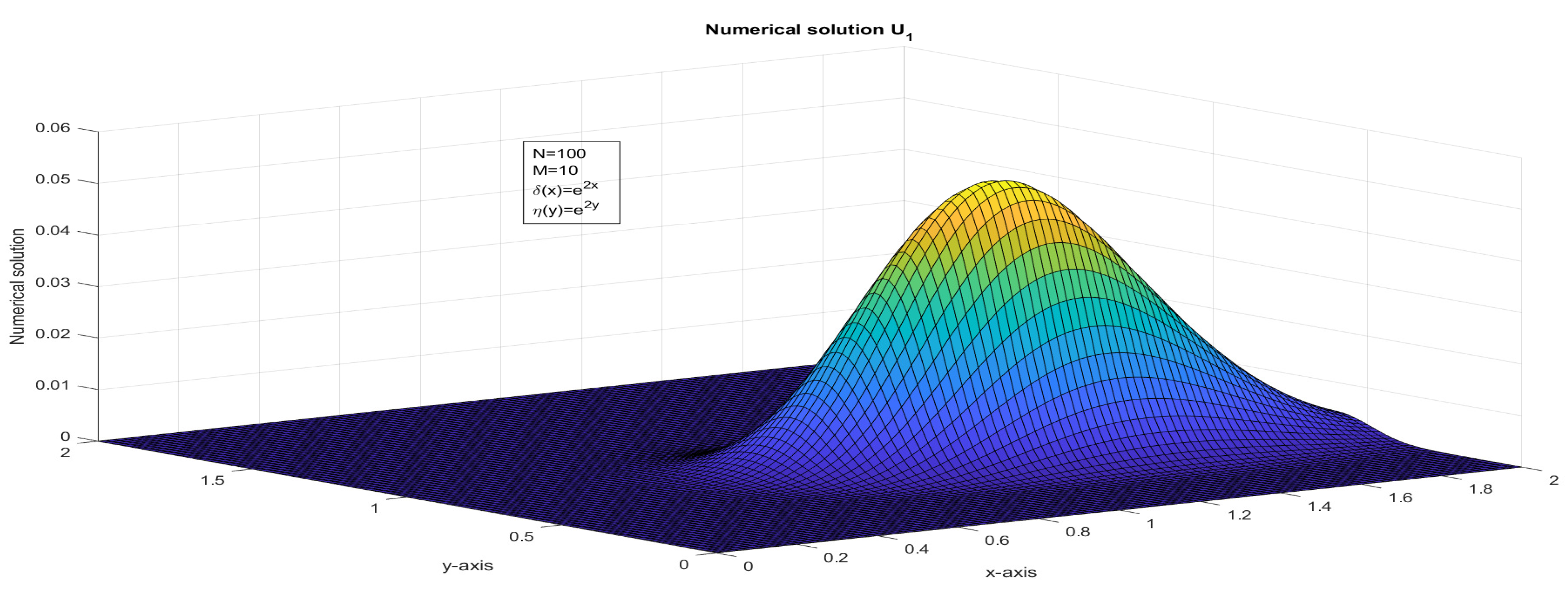
Assume that $\delta =1,\eta =1$. The two-dimensional impulse propagates in the solution due to the presence of the delay term. Numerical solutions are plotted in Figure 1 and Figure 2 and maximum point-wise errors are plotted in Figure 7 and Figure 8. The maximum point-wise errors are given in Table 1 and Table 2. The impulse moves in the forward direction can be found in Figure 11 and Figure 12.

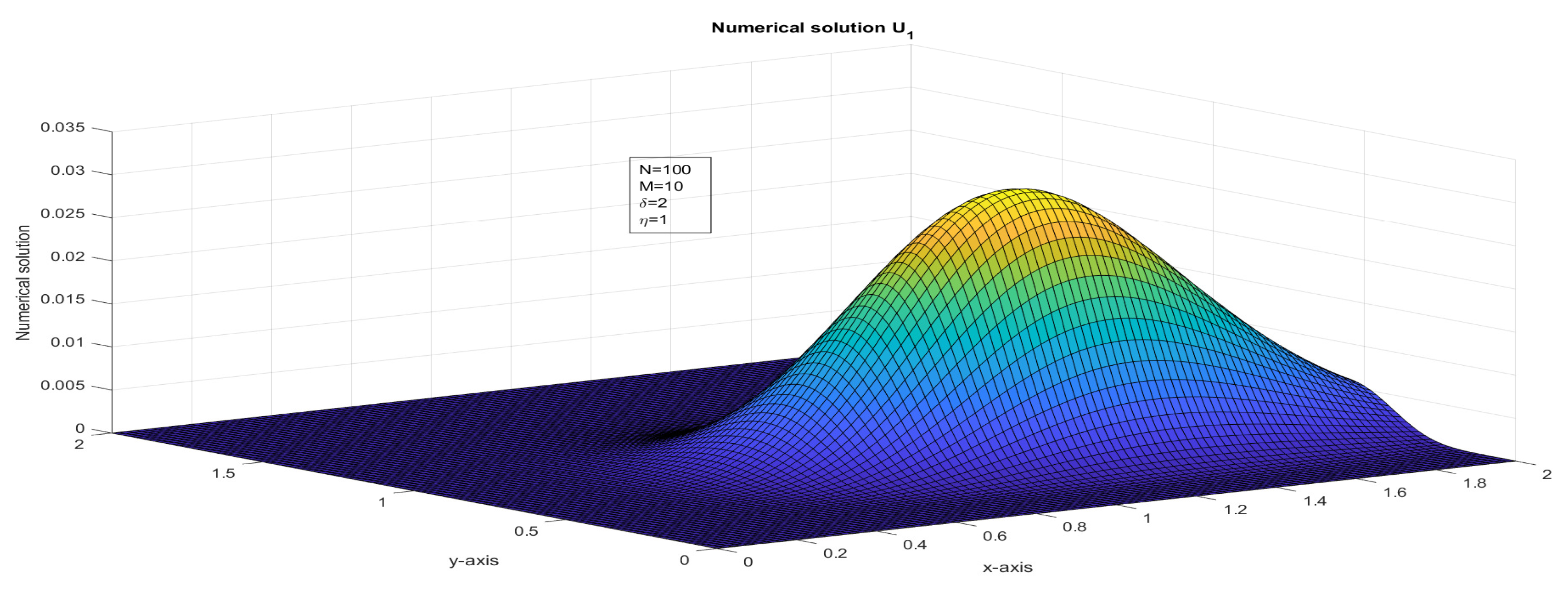
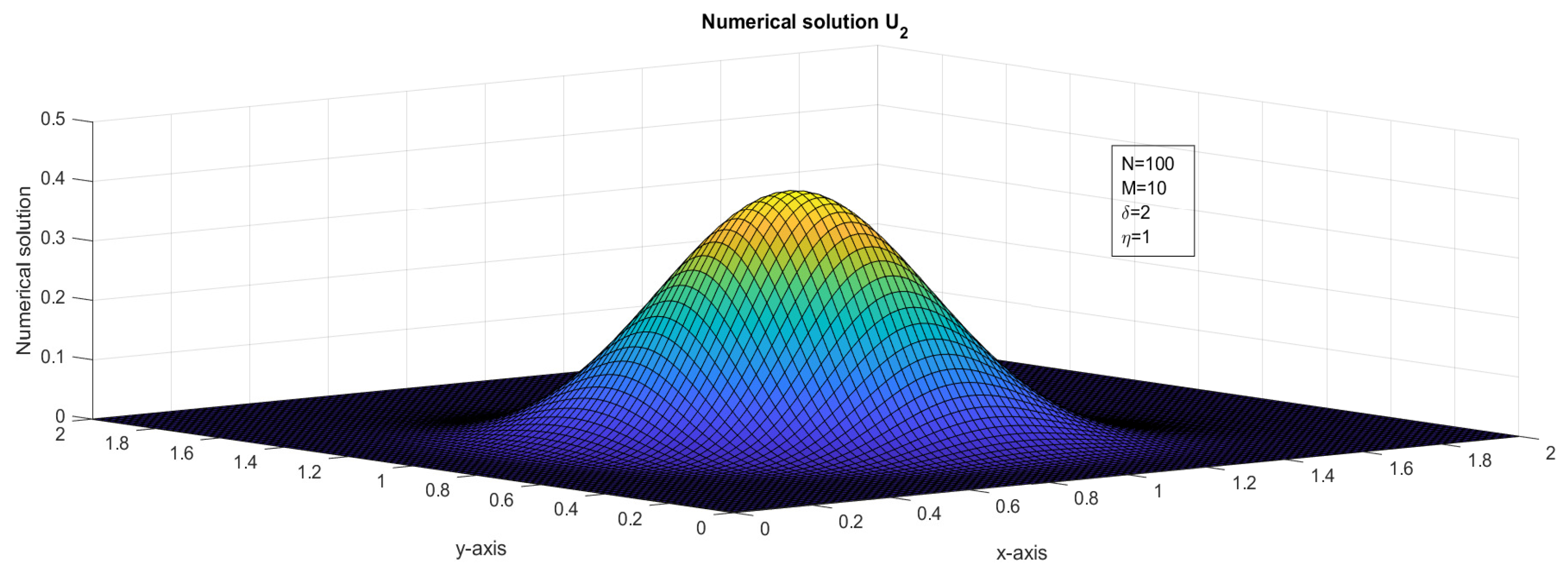
Case 2:

Assume that $\delta =2,\eta =1$. Numerical solutions are plotted in Figure 3 and Figure 4. If $\delta >\eta$, then the impulse moved in the forward x-direction, see Figure 13 and Figure 14.

Case 3:

Assume that $\delta =1,\eta =2$. Numerical solutions are plotted in Figure 5 and Figure 6. If $\eta >\delta$, then the impulse moved in the forward y-direction, see Figure 15 and Figure 16.

Example 2.

Consider the variable delay differential equation in (31)–(33).

$$\begin{array}{cc}\hfill & a_{11}={\displaystyle \frac{1+x^4+y^4}{1+3xy+x^4+y^4}},a_{12}={\displaystyle \frac{1+x^4+y^4}{1+4xy+2x^4+2y^4}},a_{21}={\displaystyle \frac{1+x^4+y^4}{1+2xy+3x^4+6y^4}},\hfill \\ & a_{22}={\displaystyle \frac{1+x^4+y^4}{1+2tx+4x^4+3y^4}},c_{11}=-1,c_{12}=-\frac{1}{2},c_{21}=-1,c_{22}=-\frac{1}{2},\hfill \\ & f_1=0=f_2,\delta (x)=e^{2x},\eta (y)=e^{2y}.\hfill \end{array}$$

Figure 9 and Figure 10 present the numerical solutions.

Figure 1. The surface plot illustrates the numerical solution, $U_1$, for Case 1 in Example 1.

Figure 2. The surface plot illustrates the numerical solution, $U_2$, for Case 1 in Example 1.

Figure 3. The surface plot illustrates the numerical solution, $U_1$, for Case 2 in Example 1.

Table 1. $U_1$— the component maximum error for Example 1 in Case 1.

	$\mathit{\delta }=1,\mathit{\eta }=1$, and N
M ↓	64	128	256	512	1024	$D_{1,t}^M$
16	8.0922 × 10${}^{-3}$	6.4475 × 10${}^{-3}$	4.2323 × 10${}^{-3}$	2.4580 × 10${}^{-3}$	1.3300 × 10${}^{-3}$	8.0922 × 10${}^{-3}$
32	5.5672 × 10${}^{-3}$	4.8529 × 10${}^{-3}$	3.3899 × 10${}^{-3}$	2.0492 × 10${}^{-3}$	1.1329 × 10${}^{-3}$	5.5672 × 10${}^{-3}$
64	3.3803 × 10${}^{-3}$	3.1249 × 10${}^{-3}$	2.2935 × 10${}^{-3}$	1.4320 × 10${}^{-3}$	8.0661 × 10${}^{-4}$	3.3803 × 10${}^{-3}$
128	1.8814 × 10${}^{-3}$	1.7998 × 10${}^{-3}$	1.3716 × 10${}^{-3}$	8.7893 × 10${}^{-4}$	5.0466 × 10${}^{-4}$	1.8814 × 10${}^{-3}$
256	9.9549 × 10${}^{-4}$	9.7438 × 10${}^{-4}$	7.5796 × 10${}^{-4}$	4.9483 × 10${}^{-4}$	3.1548 × 10${}^{-4}$	9.9549 × 10${}^{-4}$
$D_{1,x,y}^N$	8.0922 × 10${}^{-3}$	6.4475 × 10${}^{-3}$	4.2323 × 10${}^{-3}$	2.4580 × 10${}^{-3}$	1.3300 × 10${}^{-3}$	-

Table 1. $U_1$— the component maximum error for Example 1 in Case 1.

	$\mathit{\delta }=1,\mathit{\eta }=1$, and N
M ↓	64	128	256	512	1024	$D_{1,t}^M$
16	8.0922 × 10${}^{-3}$	6.4475 × 10${}^{-3}$	4.2323 × 10${}^{-3}$	2.4580 × 10${}^{-3}$	1.3300 × 10${}^{-3}$	8.0922 × 10${}^{-3}$
32	5.5672 × 10${}^{-3}$	4.8529 × 10${}^{-3}$	3.3899 × 10${}^{-3}$	2.0492 × 10${}^{-3}$	1.1329 × 10${}^{-3}$	5.5672 × 10${}^{-3}$
64	3.3803 × 10${}^{-3}$	3.1249 × 10${}^{-3}$	2.2935 × 10${}^{-3}$	1.4320 × 10${}^{-3}$	8.0661 × 10${}^{-4}$	3.3803 × 10${}^{-3}$
128	1.8814 × 10${}^{-3}$	1.7998 × 10${}^{-3}$	1.3716 × 10${}^{-3}$	8.7893 × 10${}^{-4}$	5.0466 × 10${}^{-4}$	1.8814 × 10${}^{-3}$
256	9.9549 × 10${}^{-4}$	9.7438 × 10${}^{-4}$	7.5796 × 10${}^{-4}$	4.9483 × 10${}^{-4}$	3.1548 × 10${}^{-4}$	9.9549 × 10${}^{-4}$
$D_{1,x,y}^N$	8.0922 × 10${}^{-3}$	6.4475 × 10${}^{-3}$	4.2323 × 10${}^{-3}$	2.4580 × 10${}^{-3}$	1.3300 × 10${}^{-3}$	-

Figure 4. The surface plot illustrates the numerical solution, $U_2$, for Case 2 in Example 1.

Figure 5. The surface plot illustrates the numerical solution, $U_1$, for Case 3 in Example 1.

Figure 6. The surface plot illustrates the numerical solution, $U_2$, for Case 3 in Example 1.

Table 2. $U_2$— the component maximum error for Example 1 in Case 1.

	$\mathit{\delta }=1,\mathit{\eta }=1$, and N
M ↓	64	128	256	512	1024	$D_{2,t}^M$
16	6.8702 × 10${}^{-2}$	4.4892 × 10${}^{-2}$	2.6181 × 10${}^{-2}$	1.4221 × 10${}^{-2}$	7.4248 × 10${}^{-3}$	6.8702 × 10${}^{-2}$
32	4.0786 × 10${}^{-2}$	2.7619 × 10${}^{-2}$	1.6487 × 10${}^{-2}$	9.0944 × 10${}^{-3}$	4.7898 × 10${}^{-3}$	4.0786 × 10${}^{-2}$
64	2.2413 × 10${}^{-2}$	1.5539 × 10${}^{-2}$	9.4426 × 10${}^{-3}$	5.2683 × 10${}^{-3}$	2.7922 × 10${}^{-3}$	2.2413 × 10${}^{-2}$
128	1.1778 × 10${}^{-2}$	8.2741 × 10${}^{-3}$	5.0898 × 10${}^{-3}$	2.8575 × 10${}^{-3}$	1.5196 × 10${}^{-3}$	1.1778 × 10${}^{-2}$
256	6.0411 × 10${}^{-3}$	4.2797 × 10${}^{-3}$	2.6459 × 10${}^{-3}$	1.4907 × 10${}^{-3}$	7.9392 × 10${}^{-4}$	6.0411 × 10${}^{-3}$
$D_{2,x,y}^N$	6.8702 × 10${}^{-2}$	4.4892 × 10${}^{-2}$	2.6181 × 10${}^{-2}$	1.4221 × 10${}^{-2}$	7.4248 × 10${}^{-3}$	-

Table 2. $U_2$— the component maximum error for Example 1 in Case 1.

	$\mathit{\delta }=1,\mathit{\eta }=1$, and N
M ↓	64	128	256	512	1024	$D_{2,t}^M$
16	6.8702 × 10${}^{-2}$	4.4892 × 10${}^{-2}$	2.6181 × 10${}^{-2}$	1.4221 × 10${}^{-2}$	7.4248 × 10${}^{-3}$	6.8702 × 10${}^{-2}$
32	4.0786 × 10${}^{-2}$	2.7619 × 10${}^{-2}$	1.6487 × 10${}^{-2}$	9.0944 × 10${}^{-3}$	4.7898 × 10${}^{-3}$	4.0786 × 10${}^{-2}$
64	2.2413 × 10${}^{-2}$	1.5539 × 10${}^{-2}$	9.4426 × 10${}^{-3}$	5.2683 × 10${}^{-3}$	2.7922 × 10${}^{-3}$	2.2413 × 10${}^{-2}$
128	1.1778 × 10${}^{-2}$	8.2741 × 10${}^{-3}$	5.0898 × 10${}^{-3}$	2.8575 × 10${}^{-3}$	1.5196 × 10${}^{-3}$	1.1778 × 10${}^{-2}$
256	6.0411 × 10${}^{-3}$	4.2797 × 10${}^{-3}$	2.6459 × 10${}^{-3}$	1.4907 × 10${}^{-3}$	7.9392 × 10${}^{-4}$	6.0411 × 10${}^{-3}$
$D_{2,x,y}^N$	6.8702 × 10${}^{-2}$	4.4892 × 10${}^{-2}$	2.6181 × 10${}^{-2}$	1.4221 × 10${}^{-2}$	7.4248 × 10${}^{-3}$	-

Figure 7. $U_1$—the maximum point-wise error of Example 1 for Case 1.

Figure 8. $U_2$—the maximum point-wise error of Example 1 for Case 1.

Figure 9. The surface plot illustrates the numerical solution, $U_1$, of Example 2.

Figure 10. The surface plot illustrates the numerical solution, $U_2$, of Example 2.

Figure 11. The surface plot illustrates the numerical solution, $U_1$, for Case 1 in Example 1.

Figure 12. The surface plot illustrates the numerical solution, $U_2$, for Case 1 in Example 1.

Figure 13. The surface plot illustrates the numerical solution, $U_1$, for Case 2 in Example 1.

Figure 14. The surface plot illustrates the numerical solution, $U_2$, for Case 2 in Example 1.

Figure 15. The surface plot illustrates the numerical solution, $U_1$, for Case 3 in Example 1.

Figure 16. The surface plot illustrates the numerical solution, $U_2$, for Case 3 in Example 1.

8. Conclusions

In this paper, we presented an investigation of a two-dimensional system of first-order hyperbolic delay partial differential equations (HDPDEs). Our study involved a comprehensive analysis of the theoretical aspects of the system, as well as the development of numerical methods for approximating its solution. To achieve this, we employed a fractional-step method with a finite difference scheme in discretizing the spatial derivatives of the problem. In addition to the theoretical analysis, we developed numerical methods for approximating the solution of the system. The fractional-step method with a finite difference scheme was shown to be a reliable and efficient approach for approximating the solution of the system. We established the stability of our numerical method under suitable conditions. The numerical analysis of the fractional-step method with a finite difference scheme revealed that the error estimates in both space and time were almost first-order. We used a rigorous mathematical framework to analyze the error estimates in both spatial and temporal discretization. We also established the consistency and convergence of the numerical method. If $x_f\ne r\delta$ and $y_f\ne r\eta$, then the interval $[0,x_f]$ and $[0,y_f]$ was divided with different mesh sizes. If $x_q\le x_i-\delta \le x_{q+1}$ and $y_p\le y_j-\eta \le y_{p+1}$, then a bilinear interpolation [36] of $U_{k,q,p}$, $U_{k,q+1,p}$, $U_{k,q,p+1}$, and $U_{k,q+1,p+1}$ was applied to approximate $u_k(x_i-\delta ,y_j-\eta ,t_{n+1})$. The stability analysis and truncation error analysis were crucial components of the investigation of the two-dimensional system of first-order HDPDEs. We carefully derived the stability criteria for the fractional-step method with a finite difference scheme, which ensured that the numerical solution remained stable as the time step and grid spacing varied. We also conducted a thorough analysis of the truncation error to identify the sources of error in the numerical approximation. As discussed in [10,15], for fixed $\delta$ and $\eta$, the impulse moved in the forward direction, see Figure 11 and Figure 12. For fixed $\eta$ and an increased value of $\delta >\eta$, the impulse moved in the forward x-direction, see Figure 13 and Figure 14. For fixed $\delta$ and an increased value of $\eta >\delta$, the impulse moved in the forward y-direction, see Figure 15 and Figure 16. In Figure 13, Figure 14, Figure 15 and Figure 16, the range of x and y was taken as $[0,8]$ in order to show the explicit transverse of the impulses. An application of the variable delay problem is considered and a numerical solution is presented in Figure 9 and Figure 10.

References

- Alexander, V.R.; Wu, J. A non-local PDE model for population dynamics with state-selective delay: Local theory and global attractors. J. Comput. Appl. Math. 2006, 190, 99–113. [Google Scholar]
- Al-Mutib, A.N. Stability properties of numerical methods for solving delay differential equations. J. Comput. Appl. Math. 1984, 10, 71–79. [Google Scholar] [CrossRef]
- Bellen, A.; Zennaro, M. Numerical Methods for Delay Differential Equations; Oxford University Press: Oxford, UK, 2003. [Google Scholar]
- Wu, J. Theory and Applications of Partial Functional Differential Equations; Springer: New York, NY, USA, 1996. [Google Scholar]
- Karthick, S.; Mahendran, R.; Subburayan, V. Method of lines and Runge-Kutta method for solving delayed one dimensional transport equation. J. Math. Comput. Sci. 2023, 28, 270–280. [Google Scholar] [CrossRef]
- Tunç, O.; Tunç, C.; Wang, Y. Delay-dependent stability, integrability and boundedeness criteria for delay differential systems. Axioms 2021, 10, 138. [Google Scholar] [CrossRef]
- Tunç, O.; Tunç, C. Solution estimates to Caputo proportional fractional derivative delay integro-differential equations. Rev. Real Acad. Cienc. Exactas Fís. Nat. Ser. A Mat. 2023, 117, 12. [Google Scholar] [CrossRef]
- Stein, R.B. A theoretical analysis of neuronal variability. Biophys. J. 1965, 5, 173–194. [Google Scholar] [CrossRef]
- Stein, R.B. Some models of neuronal variability. Biophys. J. 1967, 7, 37–68. [Google Scholar] [CrossRef]
- Sharma, K.K.; Singh, P. Hyperbolic partial differential-difference equation in the mathematical modelling of neuronal firing and its numerical solution. Appl. Math. Comput. 2008, 201, 229–238. [Google Scholar]
- Singh, P.; Sharma, K.K. Finite difference approximations for the first-order hyperbolic partial differential equation with point-wise delay. Int. J. Pure Appl. Math. 2011, 67, 49–67. [Google Scholar]
- Singh, P.; Sharma, K.K. Numerical solution of first-order hyperbolic partial differential-difference equation with shift. Numer. Methods Partial Differ. Equ. 2010, 26, 107–116. [Google Scholar] [CrossRef]
- Karthick, S.; Subburayan, V. Finite Difference Methods with Interpolation for First-Order Hyperbolic Delay Differential Equations. Springer Proc. Math. Stat. 2021, 368, 147–161. [Google Scholar]
- Karthick, S.; Subburayan, V. Finite difference methods with linear interpolation for solving a coupled system of hyperbolic delay differential equations. Int. J. Math. Model. Numer. Optim 2022, 12, 370–389. [Google Scholar] [CrossRef]
- Karthick, S.; Subburayan, V.; Agrwal, R.P. Stable Difference Schemes with Interpolation for Delayed One-Dimensional Transport Equation. Symmetry 2022, 14, 1046. [Google Scholar]
- Fridmana, E.; Orlov, Y. Exponential stability of linear distributed parameter systems with time-varying delays. Automatica 2009, 45, 194–201. [Google Scholar] [CrossRef]
- Smith, G.D. Numerical Solution of Partial Differential Equations: Finite Difference Methods; Oxford University Press: Oxford, UK, 1985. [Google Scholar]
- Strikwerda, J.C. Finite Difference Schemes and Partial Differential Equations; SIAM: Philadelphia, PA, USA, 2004. [Google Scholar]
- Islam, S.; Alam, M.; Al-Asad, M.; Tunç, C. An analytical technique for solving new computational of the modified Zakharov-Kuznetsov equation arising in electrical engineering. J. Appl. Comput. Mech. 2021, 7, 715–726. [Google Scholar]
- Alam, M.N.; Tunc, C. An analytical method for solving exact solutions of the nonlinear Bogoyavlenskii equation and the nonlinear diffusive predator–prey system. Alex. Eng. J. 2016, 55, 1855–1865. [Google Scholar] [CrossRef]
- Jiwari, R. Lagrange interpolation and modified cubic B-spline differential quadrature methods for solving hyperbolic partial differential equations with Dirichlet and Neumann boundary conditions. Comput. Phys. Commun. 2015, 193, 55–65. [Google Scholar] [CrossRef]
- Jiwari, R.; Pandit, S.; Mittal, R. A differential quadrature algorithm to solve the two dimensional linear hyperbolic telegraph equation with Dirichlet and Neumann boundary conditions. Appl. Math. Comput. 2012, 218, 7279–7294. [Google Scholar] [CrossRef]
- Pandit, S.; Kumar, M.; Tiwari, S. Numerical simulation of second-order one dimensional hyperbolic telegraph equation. Comput. Phys. Commun. 2015, 187, 83–90. [Google Scholar] [CrossRef]
- Protter, M.H.; Weinberger, H.F. Maximum Principles in Differential Equations; Springer Science and Business Media: New York, NY, USA, 2012. [Google Scholar]
- Mizohata, S.; Murthy, M.V.; Singbal, B.V. Lectures on Cauchy Problem; Tata Institute of Fundamental Research: Bombay, India, 1965; Volume 35. [Google Scholar]
- Peaceman, D.W.; Rachford, H.H. The numerical solution of parabolic and elliptic differential equations. SIAM J. Comput. 1955, 3, 28–41. [Google Scholar] [CrossRef]
- Thomas, B.G.; Samarasekera, I.V.; Brimacombe, J.K. Comparison of numerical modeling techniques for complex, two-dimensional, transient heat-conduction problems. Metall. Trans. B 1984, 15, 307–318. [Google Scholar] [CrossRef]
- Araújo, A.; Neves, C.; Sousa, E. An alternating direction implicit method for a second-order hyperbolic diffusion equation with convection. Appl. Math. Comput. 2014, 239, 17–28. [Google Scholar] [CrossRef]
- Clavero, C.; Jorge, J.C.; Lisbona, F. A uniformly convergent scheme on a nonuniform mesh for convection–diffusion parabolic problems. J. Comput. Appl. Math. 2003, 154, 415–429. [Google Scholar] [CrossRef]
- Clavero, C.; Jorge, J.C.; Lisbona, F.; Shishkin, G.I. An alternating direction scheme on a nonuniform mesh for reaction-diffusion parabolic problems. IMA J. Numer. Anal. 2000, 20, 263–280. [Google Scholar] [CrossRef]
- Majumdar, A.; Natesan, S. Alternating direction numerical scheme for singularly perturbed 2D degenerate parabolic convection-diffusion problems. Appl. Math. Comput. 2017, 313, 453–473. [Google Scholar] [CrossRef]
- Avudai Selvi, P.; Ramanujam, N. A parameter uniform difference scheme for singularly perturbed parabolic delay differential equation with Robin type boundary condition. Appl. Math. Comput. 2017, 296, 101–115. [Google Scholar] [CrossRef]
- Subburayan, V.; Ramanujam, N. An asymptotic numerical method for singularly perturbed convection-diffusion problems with a negative shift. Neural Parallel Sci. Comput. 2013, 21, 431–446. [Google Scholar]
- Walter, A. Strauss, Partial Differential Equations an Introduction; John Wiley & Sons, Inc.: New York, NY, USA, 2008. [Google Scholar]
- Subburayan, V.; Natesan, S. Parameter Uniform Numerical Method for Singularly Perturbed 2D Parabolic PDE with Shift in Space. Mathematics 2022, 10, 3310. [Google Scholar] [CrossRef]
- Zadorin, A.I. Approaches to constructing two-dimensional interpolation formulas in the presence of boundary layers. J. Phys. Conf. Ser. 2022, 2182, 012036. [Google Scholar] [CrossRef]
- Miller, J.J.H.; O’Riordan, E.; Shishkin, G.I. Fitted Numerical Methods for Singular Perturbation Problems: Error Estimates in the Maximum Norm for Linear Problems in One and Two Dimensions; World Scientific: Singapore, 2012. [Google Scholar]
- Varah, J.M. A lower bound for the smallest singular value of a matrix. Linear Algebra Its Appl. 1975, 11, 3–5. [Google Scholar] [CrossRef]
- Agarwal, R.P.; Chow, Y.M. Finite-difference methods for boundary-value problems of differential equations with deviating arguments. Comput. Method. Appl. Math. 1986, 12, 1143–1153. [Google Scholar] [CrossRef]
- Jain, R.K.; Agarwal, R.P. Finite difference method for second order functional differential equations. J. Math. Phys. Sci. 1973, 7, 301–316. [Google Scholar]
Disclaimer/Publisher’s Note: The statements, opinions and data contained in all publications are solely those of the individual author(s) and contributor(s) and not of MDPI and/or the editor(s). MDPI and/or the editor(s) disclaim responsibility for any injury to people or property resulting from any ideas, methods, instructions or products referred to in the content. |
© 2023 by the authors. Licensee MDPI, Basel, Switzerland. This article is an open access article distributed under the terms and conditions of the Creative Commons Attribution (CC BY) license (https://creativecommons.org/licenses/by/4.0/).