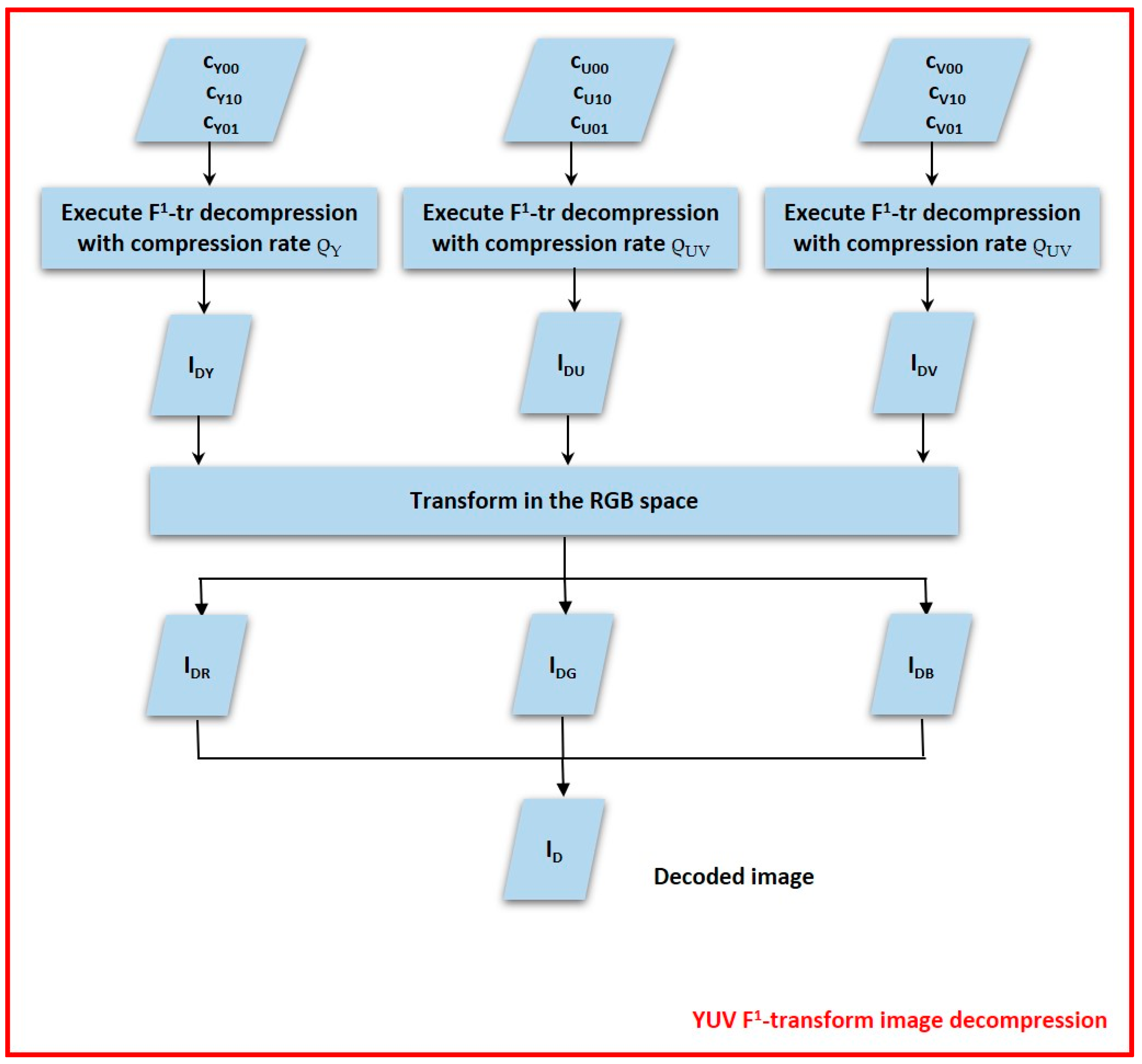
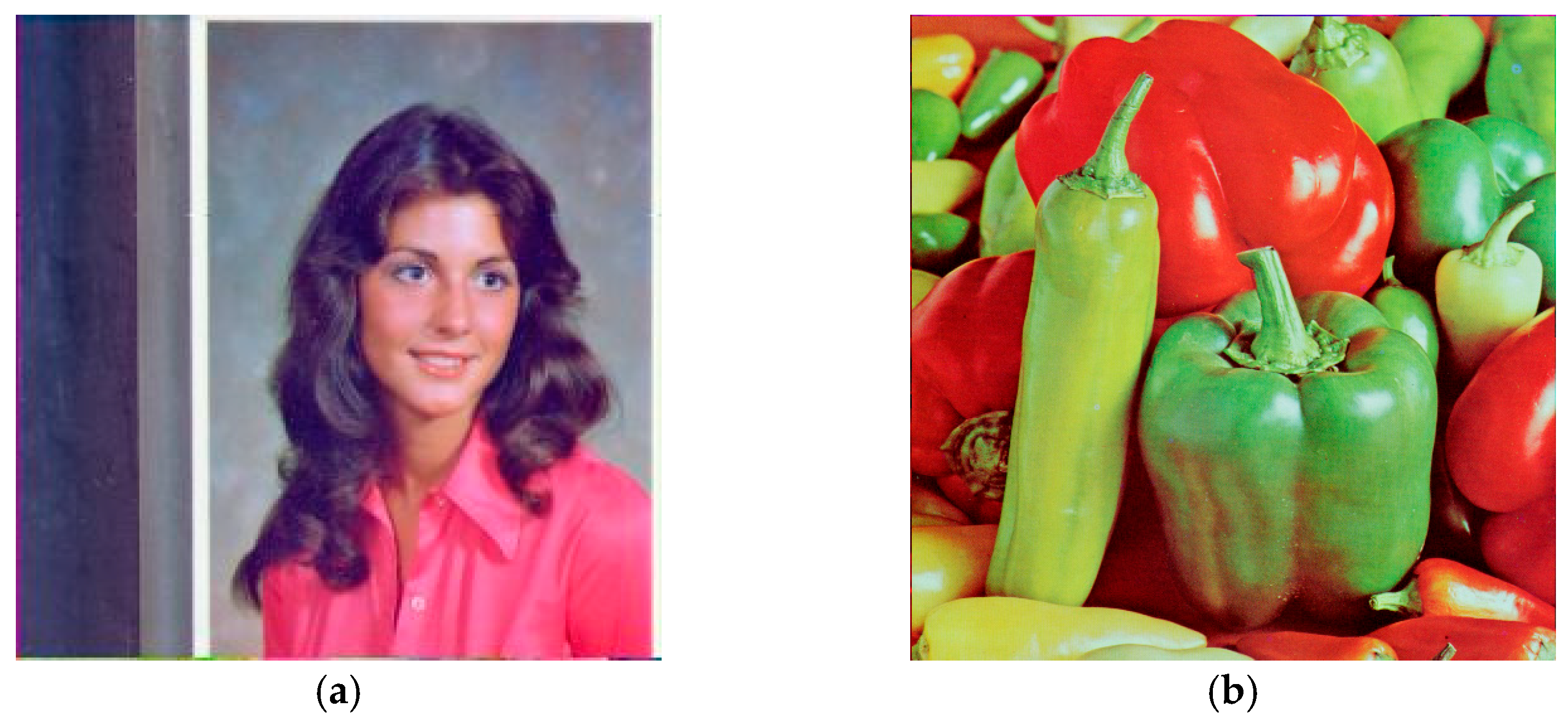
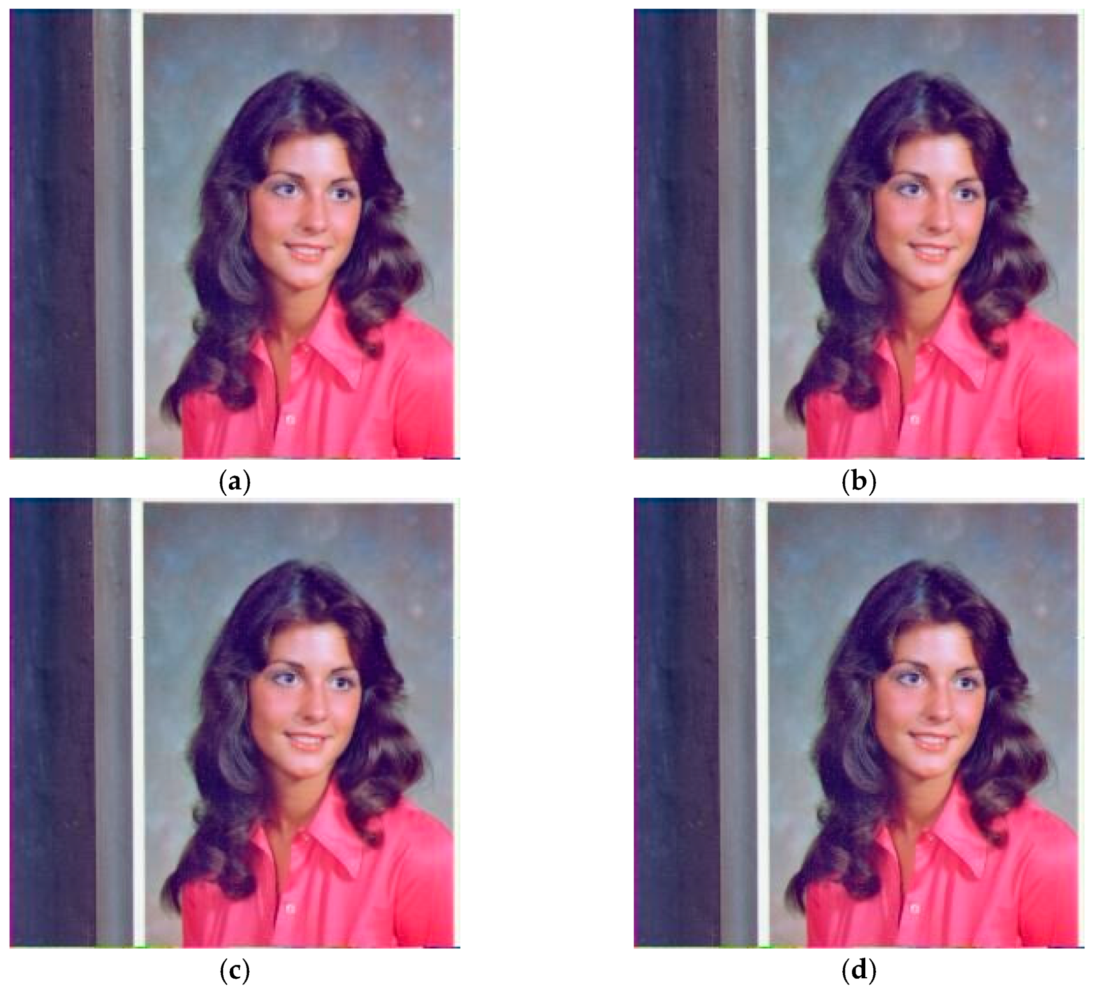
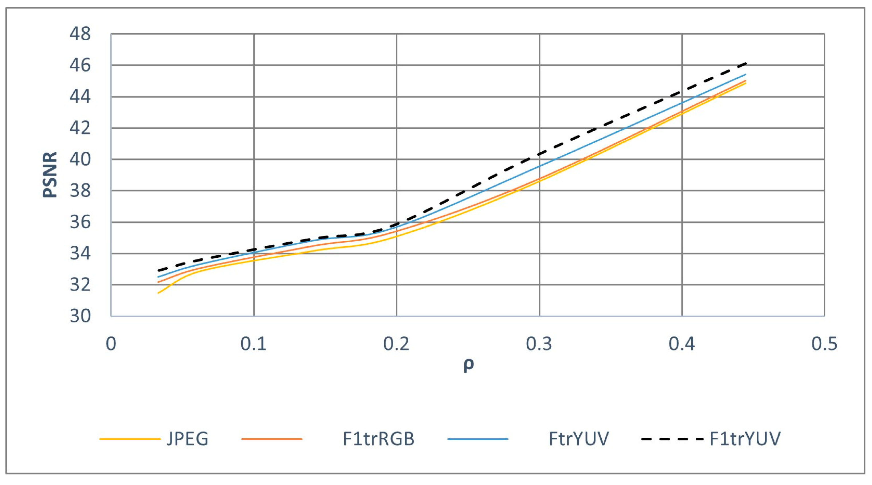
2.1. The bi-Dimensional F-Transform
Let [a, b] be a closed real interval and let {x1, x2, …, xn} be a set of points of [a, b], called nodes, such that x1 = a < x2 <…< xn = b.
Let {A1,…,An} be a family of fuzzy sets of X, where Ai: [a, b] → [0, 1]: it forms a fuzzy partition of X id the following conditions hold:
- (1)
Ai(xi) = 1 for every i =1, 2, …, n;
- (2)
Ai(x) = 0 if x∉(xi − 1, xi + 1), by setting x0 = x1 = a and xn + 1 = xn = b;
- (3)
Ai(x) is a continuous function over [a, b];
- (4)
Ai(x) is strictly increasing over [xi − 1, xi] for each i = 2, …, n;
- (5)
Ai(x) is strictly decreasing over [xi, xi + 1] for each i = 1, …, n−1;
- (6)
for every x∈[a, b].
Let . The fuzzy partition {A1, …, An} is an uniform fuzzy partition if:
- (7)
n ≥ 3;
- (8)
xi =a + h∙(i−1), for i = 1, 2, …, n;
- (9)
Ai(xi−x) = Ai(xi + x) for every x [0, h] and i = 2, …, n−1;
- (10)
Ai + 1(x) = Ai(x−h) for every x [xi, xi + 1] and i = 1, 2, …, n−1.
Let
f(x) be a continuous function over [a, b] and {A
1, A
2, …, A
n} be a fuzzy partition of [a, b]. The n-tuple F =
is called
uni-dimensional direct F-transform of
f with respect to {A
1, A
2, …, A
n} if the following holds:
The following function
defined for every x∈[a, b] as
is called the uni-dimensional inverse F-transform of the function f.
The following theorem holds (cfr. ([
7], Theorem 2)):
Theorem 1. Let f(x) be a continuous function over [a, b]. For every ε > 0 there exists an integer n(ε) and a fuzzy partition {A1, A2, …, An(ε)} of [a, b] for which holds the inequality for every x [a, b].
Now, consider the discrete case where the function f is known in a set of N points P = {p1, …, pN}, where pj ∈ [a, b], j = 1, 2, …, m. The set {p1, …, pN} is called sufficiently dense with respect to the fixed fuzzy partition {A1, A2, …, An} if for i = 1, …, n, there exists at least an index j {1, …, m} such that Ai(pj) > 0.
If the set P is sufficiently dense with respect to the fuzzy partition, we can define the
discrete direct F-transform with components given as
and the
discrete inverse F-transform as
The following theorem applied to the discrete inverse F-transform holds (cfr. ([
7], Theorem 5)):
Theorem 2. Let f(x) be a continuous function over [a, b] known in a discrete set of points P = {p1, …, pm}. For every ε > 0, there exists an integer n(ε) and a fuzzy partition {A1, A2, …, An(ε)} of [a, b], with respect to which P is sufficiently dense, for which the following inequality holds for j = 1, …, N.
According to Theorem 2, the inverse fuzzy transform (4) can be used to approximate the function f in a point.
Now, we consider functions in two variables. Let x1, x2, …, xn be a set of n nodes in [a,b] where n > 2 and x1 = a < x2 <…< xn = b, and let y1, y2, …, ym be a set of m nodes in [c,d], where m > 2 and and y1 = c < y2 <…< ym = d. Moreover, let A1,…,An: [a, b] → [0, 1] be a fuzzy partition of [a, b], B1, …, Bm: [c, d] → [0, 1] be a fuzzy partition of [c, d] and let f(x,y) be a function defined in the Cartesian product [a, b] × [c, d].
We suppose that f assumes known values in a set of points (pj, qj)∈[a, b] × [c, d], where i = 1, …, N and j = 1, …, m, where the set P = {p1, …, pN} is sufficiently dense with respect to the fuzzy partition {A1, …, An} and the set Q = {q1, …, qM} is sufficiently dense with respect to the fuzzy partition {B1, …, Bm}.
In this case, we can define the
bi-dimensional discrete F-transform of
f, given by matrix [F
hk] with entries defined as
and the
bi-dimensional discrete inverse F-transform of
f with respect to {A
1, A
2, …, A
n} and {B
1, …, B
m} defined as
2.2. The bi-Dimensional F1-Transform
This paragraph introduces the concept of higher-degree fuzzy transform or F1-transform.
Let A
h, h = 1, …, n, be the h
th fuzzy set of the fuzzy partition {A
1, …, A
n} defined in [a, b] and L
2([x
h − 1,x
h + 1]) be the Hilbert space of square-integrable functions
f,
g: [x
h − 1,x
h + 1] ⟶ R with the inner product:
Given a integer r ≥ 0, we denote with
([x
h−1,x
h+1]) a linear subspace of the Hilbert space L
2([x
h−1,x
h+1]) that has as an orthogonal basis the polynomials {
,
, …,
} constructed by applying the Gram–Schmidt ortho-normalization to the linear independent system of polynomials {1, x, x
2, …, x
r} defined in the interval [x
h−1,x
h+1]. We have the following:
The following Lemma holds (Cfr. [
7], Lemma 1):
Lemma 1. Let be the orthogonal projection of the function f on ([x
h−1,x
h+1]).
Then,where it is the h
th component of the direct Fr-transform of
f. The inverse Fr-transform of
f in a point x ∊ [a, b] is defined as
For r = 0, we have = 1 and the F0-transform is given by the F-transform in one variable ( (x) = ch,0).
For r = 1, we have
= (x − x
h) and the h
th component of the F1-transform is given as
If the function
f is known in a set of N points, P = {p
1, …, p
N}, c
h,0 and c
h,1 can be discretized in the following formulas:
The F1-transform can be extended in a bi-dimensional space. We consider the Hilbert space L
2([x
h−1, x
h+1] × [y
k−1, y
k+1]) of square-integrable functions
f: [x
h − 1, x
h + 1] × [y
k − 1,y
k + 1]→ R with the weighted inner product:
Two functions L2 ([xh−1, xh+1] × [yk−1, yk+1]) are orthogonal if .
Let f: X ⊆ R2 → Y⊆ R be a continuous bi-dimensional function defined in [a, b] × [c, d]. Let {A1, A2, …, An} be a fuzzy partition of [a, b] and {B1, B2, …, Bm} be a fuzzy partition of [c, d]. Moreover, let {(p1,q1),…, (pN,qjN)} a set of N points in which the function f is known, where (pj,qj) [a, b] × [c, d]. Let P = {p1, …, pN} be sufficiently dense with respect to the fuzzy partition {A1, …, An} and Q = {q1, …, qM} be sufficiently dense with respect to the fuzzy partition {B1, …, Bm}.
We can define the bi-dimensional direct F1-transform of
f, with components given as
where
is the component
of the bi-dimensional discrete direct F transform of
f, defined via Formula (5). The three coefficients in (17) are given as
The inverse F1-transform of
f in a point (x,y) ∊ [a, b] × [c, d] is defined as
where
is the (h,k)
th component of the bi-dimensional direct F1-transform given from Formula (16).
2.3. Coding/Decoding Images using the Bidimensional F and F1-Transforms
Let I be a gray N × M image. A pixel can be considered a data point with coordinates (i,j), where i = 1, 2, …, N and j = 1, 2, …, M: the value of this data point is given as the pixel value I(i,j). In [
8], the image is normalized in [0, 1] according to the formula R(i,j) = I(i,j)/(L-1), where L is the number of gray levels.
We can create a partition of this image in blocks of equal size N(B) × M(B), coded to a block FB of sizes n(B) × m(B), with n(B) << N(B) and m(B) << M(B), using the bi-dimensional direct F-transform.
Let {A
1, …, A
n(B)} be a fuzzy partition of the set [1,N(B)] and let {B
1,…,B
m(B)} be a fuzzy partition of the set [1,M(B))]. Each block is compressed by the bi-dimensional direct F-transform:
The coded image is reconstructed by merging all compressed blocks. Each block is decompressed using the bi-dimensional inverse F-transform. The pixel value I(i,j) in the block is approximated with the following value:
The decoded image is reconstructed by merging the decompressed blocks. The F-transform compression and decompression algorithms are shown in the pseudocode as Algorithms 1 and 2, respectively.
| Algorithm 1: F1-transform image compression |
| Input: N × M Image I with L grey levels |
| Size of the blocks of the source image N(B) × M(B) |
| Size of the compressed blocks n(B) × m(B) |
| Output: n × m compressed image IC |
Normalize the source image I in [0, 1] Partition the source image in blocks of size N(B) × M(B) For each block For h = 1 to n(B) For k = 1 to m(B) Compute the (hk)th component of the bidimensional direct F-transform by (21) Next k Next h Next block Merge the compressed blocks De-normalize the image Return the compressed n × m image IC
|
| Algorithm 2: F-transform image decompression |
| Input: n × m compressed image Ic |
| Output: N × M decoded image ID |
Normalize the compressed image in [0, 1] Partition the compressed image Ic in blocks of size n(B) × m(B) For each compressed block For i = 1 to N(B) For j = 1 to M(B) Compute the (i,j)th pixel of the decoded block by the bidimensional inverse F-transform (22) Next j Next i Next compressed block Merge the decompressed blocks De-normalize the decompressed image Return the decompressed N × M image ID
|
In [
22] an improvement in the quality of the decompressed image is accomplished using the bi-dimensional F1-transform. The blocks are compressed by using the bi-dimensional direct F1-transform:
where
The three coefficients , and are constructed by merging the coefficients of each block and finally stored, forming the output of coding process.
During the decompression process, the image is reconstructed by decompressing the block with the following bi-dimensional inverse F1-transform:
where the bi-dimensional direct F
1-transform of the block
is calculated using (23).
The decompressed blocks are merged to form the decompressed image. The F1-transform compression and decompression algorithms are shown in the pseudocode as Algorithms 3 and 4, respectively.
| Algorithm 3: F1-transform image compression |
| Input: N × M Image I with L grey levels |
| Size of the blocks of the source image N(B) × M(B) |
| Size of the compressed blocks n(B) × m(B) |
| Output: n × m matrices of the direct F1-transform coefficients , and |
Normalize the source image I in [0, 1] Partition the source image in blocks of size N(B) × M(B) For each block For h = 1 to n(B) For k = 1 to m(B) Compute the component by (24) Compute the component by (25) Compute the component by (26) Compute the (hk)th component of the bidimensional direct F1-transform by (26) Next k Next h Next block Merge the compressed blocks to obtain the n×m matrices of the coefficients , and Return the compressed n×m matrices of the coefficients , and
|
| Algorithm 4: F1-transform image decompression |
| Input: n × m matrices of the direct F1-transform coefficients coefficients , and |
| Size of the blocks of the decoded image N(B) × M(B) |
| Size of the blocks of the coded image n(B) × m(B) |
| Output: N × M decoded image ID |
Partition the F1-transform coefficients , and in blocks of size n(B) × m(B) For each compressed block For i = 1 to N(B) For j = 1 to M(B) Compute the (i,j)th pixel of the decoded block by the bidimensional inverse F1-transform (27) Next j Next i Next compressed block Merge the decompressed blocks De-normalize the decompressed image Return the decompressed N × M image ID
|

