Solving the Optimal Reactive Power Dispatch Problem through a Python-DIgSILENT Interface

Abstract

The Optimal Reactive Power Dispatch (ORPD) problem consists of finding the optimal settings of reactive power resources within a network, usually with the aim of minimizing active power losses. The ORPD is a nonlinear and nonconvex optimization problem that involves both discrete and continuous variables; the former include transformer tap positions and settings of reactor banks, while the latter include voltage magnitude settings in generation buses. In this paper, the ORPD problem is modeled as a mixed integer nonlinear programming problem and solved through two different metaheuristic techniques, namely the Mean Variance Mapping Optimization and the genetic algorithm. As a novelty, the solution of the ORPD problem is implemented through a Python-DIgSILENT interface that combines the strengths of both software. Several tests were performed on the IEEE 6-, 14-, and 39-bus test systems evidencing the applicability of the proposed approach. The results were contrasted with those previously reported in the specialized literature, matching, and in some cases improving, the reported solutions with lower computational times.

1. Introduction

Electric power systems play a key role in modern societies, since they allow us to transport energy from generation centers to loads. This is carried out through a complex infrastructure that involves centrally-dispatched generation, substations and high-voltage transmission lines. The ORPD is part of the daily operation of power systems; it consists of finding the right settings of transformer taps, reactor banks and voltage set points in generation buses, generally with the aim of minimizing active power losses [1]. The ORPD is usually solved after the unit commitment, which is the process of programming the active power generation as a function of their biding prices and limits [2,3]. The first attempts to solve the ORPD problem resorted to classical optimization techniques such as linear programming [4], quadratic programming [5] and interior point methods [6]. Although these techniques are effective for solving convex optimization problems, they do not perform well when solving Mixed Integer Nonlinear Programming (MINLP) problems. These type of problems are better handled by heuristic and metaheuristic techniques as shown in [7,8,9,10] when it is not possible to transform these into mixed-integer models.

Owing to its nature, several metaheuristic techniques have been applied to solve the ORPD problem. The main advantage of these approaches is that they are able to deal with nonconvex optimization problems involving discrete and continuous variables [11,12]. Furthermore, they do not require differentiability of the objective function or constraints, overcoming the disadvantages of classic optimization algorithms. Metaheuristic algorithms are usually inspired by natural or social phenomena. Some of these methodologies, applied to the solution of the ORPD problem, are described below.

In [13], the authors propose a gravitational search algorithm (GSA) applied to the ORPD problem. In this technique, the solution candidates are represented by masses that interact according to the law of gravity and Newton’s laws. The proposed GSA is tested on the IEEE 30-bus, 57-bus and 118-bus test systems considering minimization of active power losses, improvement of voltage profile and enhancement of voltage stability. An opposition-based GSA is developed in [14] to further improve the optimization performance of the basic GSA.

In [15], the ORPD is approached using a harmony search algorithm with the objective of minimizing power losses and improving voltage profile. This method is based on a phenomenon inspired by the improvisation process of musicians. The study is implemented on the IEEE 30-bus and 57-bus test systems, and the results obtained are compared with other techniques that include GA and Particle Swarm Optimization (PSO).

In [16,17], the authors use a particle swarm optimization (PSO) method to solve the ORPD problem considering voltage security assessment and voltage stability, respectively. The PSO is a metaheuristic inspired by the behavior of bird flocks and fish schools. Several variants of this approach have also been applied to solve the ORPD problem. In [18], three PSO variants are explored to solve the reactive power and voltage control problem. The first two are known as global and local neighborhood variants of PSO, while the third one is the coordinated aggregation PSO algorithm. In [19], the turbulent and turbulent crazy variants of PSO are also implemented. The authors perform several tests on the IEEE 57-bus and IEEE 118-bus test systems, comparing their results with other metaheuristic techniques. It was found that the performance of PSO is considerably improved when the turbulent and turbulent crazy variants are implemented, outperforming classic metaheuristic approaches. In [20], the authors proposed a hybrid fuzzy-PSO algorithm that features improved exploration and exploitation processes to approach the ORPD in real-size power systems. Test systems of up to 354 nodes were used to validate the results. This algorithm showed a better performance than the classical PSO approach.

In [21], a stochastic fractal search method is used to solve the multi-objective ORPD problem considering the minimization of power losses along with voltage deviation and a voltage stability index. In [22], the authors implemented the mean-variance mapping optimization (MVMO) algorithm to solve the ORPD problem. The effectiveness of the proposed algorithm was tested in the IEEE 30-bus test system and compared with other metaheuristic approaches.

A survey of different metaheuristic techniques applied to the ORPD problem is presented in [23]. In this paper, the authors also propose the sine–cosine algorithm to approach the ORPD problem. A validation of the proposed algorithm is carried out with differential evolution (DE) and PSO among other techniques. In [24], the authors propose an optimization algorithm based on the gradient to solve the ORPD, taking into account dispersed distributed generation in distribution networks. In [25], the authors use a hybrid fractional PSO with GSA (FPSOGSA) to solve the ORPD problem. The proposed model is validated with the IEEE 30 and IEEE 57-bus test systems with the minimization of active power transmission line losses and voltage deviation. The authors in [26] propose an entropy evolution technique implemented into FPSOGSA to further improve its performance.

In [27,28,29,30], evolutionary algorithms for addressing ORPD are presented. These algorithms are based on the postulates of biological evolution in which an initial set of individuals (solution candidates) give rise to other individuals with which they must compete in such a way that the fittest (best quality solutions) prevail over time, giving rise to new and better solutions. In [27], an evolutionary algorithm based on quantum computing is presented that seeks to jointly solve the optimal dispatch of both active and reactive power. The authors validate their approach with the IEEE 30 and 118-bus test systems comparing their results with those obtained with simulated annealing (SA) and ant colony optimization. In [28], a DE algorithm is proposed bearing in mind several objectives, including voltage stability enhancement, voltage profile improvement and losses minimization. In [31], the authors implemented a specialized GA in the DIgSILENT programming language (DPL) to solve the ORPD problem. As a main contribution, the proposed approach takes advantage of the modeling capabilities of DIgSILENT [32]. This software includes a detailed modeling of all sorts of power system elements, including generators, reactors, transmission lines and transformers. Furthermore, it counts with its own programming language that can be used to run power flow calculations with low computational time.

Other optimization techniques applied to solve the ORPD include moth–flame optimization [33], the bat optimization algorithm [34], tabu search [35,36] and the slime mold algorithm [37] among others. A detailed description of such techniques is not within the scope of this document; nonetheless, a review of metaheuristic techniques used to solve the ORPD problem can be consulted in [38].

Following the research line adopted by [31], this paper presents a Python-DIgSILENT interface to solve the ORPD problem. The proposed approach integrates the advantages of using a specialized software that allows detailed modeling of network assets and has effective power flow algorithms (DIgSILENT) with a versatile programming language that surpasses the capabilities of DPL (Python). The main contribution of this paper is the integration of this software to solve the ORPD problem in electric power systems. The ORPD problem is well known in electrical engineering for being nonlinear, nonconvex and presenting several sub-optimal solutions. The complexity of the ORPD problem largely surpasses the built-in capabilities and functionalities of the DigSILENT Power Factory software alone. Therefore, an interface with an object-oriented, high-level programming language is implemented. The main advantage of the proposed interface is the fact of counting with several optimization libraries that can be used not only to solve the ORPD problem but other optimization problems in electric power systems. To show the applicability of the proposed approach and for comparative purposes with [31], several tests were carried out with the IEEE 6, IEEE 14 and IEEE 39-bus test system with two metaheuristic techniques developed in Python programming language, namely MVMO and GA.

The rest of the document is organized as follows: Section 2 presents the general mathematical formulation of the ORPD problem in power systems. Section 3 describes the Python-DIgSILENT interface developed in this research work. Section 4 presents the main characteristics of the test systems that feature 6, 14 and 39 buses, respectively. Section 5 presents the tests and results where the Python-DIgSILENT interface is used to solve the ORPD using MVMO and GA in three benchmark IEEE test systems. Finally, the conclusions are discussed in Section 6.

2. Mathematical Modeling of the ORPD Problem

Within the ORPD problem the continuous variables are related to generation of active and reactive power as well as voltage magnitudes. On the other hand, the integer variables are related to transformer tap positions as well as reactive power compensators. The mathematical modeling of the ORPD problem adopted in this research is described in the next subsections [39].

2.1. Objective Function

Several objective functions may be envisaged when approaching the ORPD, such as enhancement of voltage profile, amelioration of voltage stability or minimization of power losses, the last one being the most common. Equation (1) presents the objective function considered in this paper which consists on minimizing the total active power losses for a given operative scenario. In this case, $p_{\mathrm{loss}}$ represents the value of the objective function; $v_m$ and $v_k$ are the magnitudes of voltages at buses m and k with angles ${\theta }_m$ and ${\theta }_k$, respectively; $Y_{km}\left(t_a\right)$ is the admittance magnitude associated with buses k and m. This admittance depends on the values of the transformer taps $t_a$, and its angle is given by ${\varphi }_{km}\left(t_a\right)$. Finally, $\mathcal{N}$ indicates the set of network buses.

$$\begin{array}{c}\hfill min{p}_{\mathrm{loss}}=\sum _{k\in \mathcal{N}}\sum _{m\in \mathcal{N}}{Y}_{km}\left(t_a\right)v_k{v}_{m}cos\left({\theta }_k-{\theta }_m-{\varphi }_{km}\left(t_a\right)\right),\end{array}$$

(1)

Note that the admittance matrix is a function of the transformers tap positions. This is due to the fact that such devices change the operational state of the transformer based on the fact that its capacities and inductive effects modify the reactance components of the admittance matrix [40].

2.2. Equality Constraints

The ORPD is subject to active and reactive power balance restrictions at each bus given by Equations (2) and (3), respectively.

$$p_k^g-p_k^d=\sum _{m\in \mathcal{N}}{Y}_{km}\left(t_a\right)v_k{v}_{m}cos\left({\theta }_k-{\theta }_m-{\varphi }_{km}\left(t_a\right)\right),\forall k\in \mathcal{N}$$

(2)

$$q_k^g-q_k^d+q_k^c\left(c_j\right)-q_k^l\left(r_l\right)=\sum _{m\in \mathcal{N}}{Y}_{km}\left(t_a\right)v_k{v}_{m}sin\left({\theta }_k-{\theta }_m-{\varphi }_{km}\left(t_a\right)\right),\forall k\in \mathcal{N}$$

(3)

In this case, $p_k^g$ and $q_k^g$ indicate the active and reactive power injections given by the generator located at node k; $p_k^d$ and $q_k^d$ indicate the active and reactive power demands at bus k; $q_k^c\left(c_j\right)$ indicates the reactive power injection provided by a capacitor bank located at bus k with the tap position $c_j$; $q_k^l\left(r_l\right)$ is the reactive power absorption of a reactor located at bus k with a tap position given by $r_l$.

2.3. Inequality Constraints

Equations (4) and (5) represent voltage and reactive power generation limits for all the generators. Constraints given by Equations (6)–(8) enforce limits on the taps of capacitor banks, reactors and power transformers. Finally, Equation (9) limits the voltage magnitudes in all buses.

$$v_i^{g,min}\le v_i^g\le v_i^{g,max},\forall i\in \mathcal{G}$$

(4)

$$q^{g,min}\le q_k^g\le q_k^{g,max},\forall k\in \mathcal{N}$$

(5)

$$c_j^{min}\le c_j\le c_j^{max},\forall j\in \mathcal{C}$$

(6)

$$r_l^{min}\le r_l\le r_l^{max},\forall l\in \mathcal{L}$$

(7)

$$t_a^{min}\le t_a\le t_a^{max},\forall a\in \mathcal{T}$$

(8)

$$v_k^{min}\le v_k\le v_k^{max},\forall k\in \mathcal{N}$$

(9)

In this case, $v_i^g$ is the voltage magnitude of the ith generator; $c_j$ is the tap position of capacitor bank j; $r_l$ is the tap position of the lth reactor compensator; $v_i^{g,max}$ and $v_i^{g,min}$ represent the bounds (upper and lower, respectively) related to voltage variables at generation buses; $q_k^{g,max}$ and $q_k^{g,min}$ represent upper and lower limits of power generation at bus k; $c_j^{max}$ and $c_j^{min}$ indicate the maximum and minimum bounds of the tap positions at the jth capacitor bank; $r_l^{max}$ and $r_l^{min}$ indicate the maximum and minimum limits of the tap positions at the lth reactor; $t_a^{max}$ and $t_a^{min}$ indicate the maximum and minimum limits of the tap position related to the ath transformer; finally, $v_k^{max}$ and $v_k^{min}$ are the upper and lower voltage limits associated to the kth node.

Note that the injections of reactive power provided by the capacitor banks as well as the absorption of reactive power of the reactors are a function of the tap positions of these devices [22,41]. Furthermore, the tap modeling can be performed as a continuous variable or by means of discrete stages, using the former results in a nonlinear optimization model, while using the later results in a general MINLP problem [42].

The optimization problem indicated by Equations (1)–(9) is nonlinear and nonconvex. This is evident in Equations (2) and (3) which involve trigonometric functions as well as a nonlinear relation of the admittance matrix with the transformer taps [21,43]. Moreover, the presence of integer variables makes the problem even more complex. As evidenced in the literature review, these types of problems are usually solved through metaheuristic techniques instead of classical optimization methods. In this paper we implemented two metaheuristic techniques to approach the ORPD problem through a Python-DIgSILENT interface, namely MVMO and GA.

3. Python-DIgSILENT Interface

This section presents the main characteristics of the Python-DIgSILENT interface to face the ORPD problem through the combination of the Newton–Raphson load flow solution in DIgSILENT [31], and the metaheuristic optimization techniques, i.e., the MVMO and the GA, implemented in the Python programming environment [44].

3.1. DIgSILENT Power Factory Software

DIgSILENT PowerFactory is one of the most popular power system software available in the market. It is widely used by electricity companies for analyzing generation, distribution and transmission and is also used by industrial systems. DIgSILENT covers a full range of functions, from standard features to advanced and highly sophisticated applications, that includes real-time simulation, renewable energy, distributed generation, and performance monitoring for the supervision and testing of electrical systems. DIgSILENT is easy to use, is Windows compatible and integrates flexible and reliable system modeling capabilities along with sophisticated algorithms and a unique database concept [45]. In addition, with its flexibility for scripting and interfaces, it is suited for highly automated and integrated solutions in business applications.

To sum up, DIgSILENT PowerFactory was selected in this research work bearing in mind the following criteria: (1) it counts with its own programming language (DPL) that can be used to compute several load flows with low computational effort, (2) it allows detailed modeling of power system devices that includes transmission lines, transformers, reactors, as well as generators and induction motors, and (3) the integration of power system elements is straightforward for load flow analyses [46].

3.2. Python Programming Language

Python is an open-source, cross-platform programming language whose philosophy emphasizes code readability. It is an object-oriented, high-level programming language that features fewer steps compared to Java and C [47]. Python was initially founded in 1991 by developer Guido Van Rossum. Due to its readability along with dynamic typing and binding, it has rapidly become popular among programmers, and currently it is among the fastest growing languages in the world. One of the advantages of Python programming language is counting with a very active community. Many organizations such as Google, Yahoo and YouTube have adopted Python.

Python has been integrated with other languages used for solving optimization problems, among which are those related to power systems. Python’s versatility, ease of adaptation, integration and robustness have given it a place in the formulation of optimization problems, either as a main language or as a complement. The specialized literature presents diverse examples of the use of tools developed in Python that allow modeling, use of specialized analysis methods and easy integration with external methodologies for solving power system problems [48,49]. In addition, examples of power system problem solving, such as electrical planning [50], weak node detection using statistical methods [51] and optimal reactive power dispatch [52] have been implemented using this programming language.

3.3. Design of the Python-DIgSILENT Interface

The Python-DIgSILENT interface integrates all the features of Python (libraries, readable code, documentation and support community) and allows access from Python to all the functionality that DIgSILENT PowerFactory provides as power system modeling software. The interface integrates Python libraries that focus on optimization, data analytics and machine learning in conjunction with the detailed power system modeling that allows DIgSILENT PowerFactory. An example of the interface is depicted in Figure 1 where power losses of a transmission system are computed.

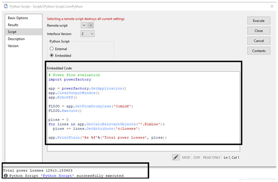
Figure 1. Example of an AC load flow loss calculation (evaluated using Newton–Raphson) in Python-DIgSILENT script software.

Figure 2 shows how to perform the same calculation using the standard DPL (DIgSILENT Programming Language) form of programming, which involves an understanding of the features of writing code, necessitates more time in application development and does not have the aforementioned benefits of using a programming language such as Python.

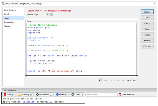
Figure 2. Example of an AC load flow loss calculation (evaluated using Newton–Raphson) in DIgSILENT Programming Language.

The workflow between DigSILENT and the Python programming language is shown in Figure 3. In this case, the software DigSILENT allows integration with the Python executable via ComPython objects. Using Python, the integration library is loaded, which allows the connection with the DigSILENT program and with the optimization libraries.

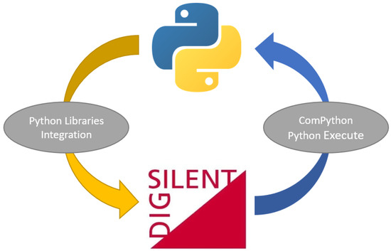
Figure 3. DIgSILENT Power Factory and Python Programming Language workflow.

3.4. Implementation of Optimization Libraries

The solution of the proposed optimization problem involved the use of open-source Python libraries. In this case, the MVMO [53] and PyMoo [54] libraries were used. These libraries allow the assignment of constraint functions, the objective function, the control variables and the input parameters (initial population, initial control variables, number of mutations and number of iterations). The PyMoo library contains different optimization algorithms. In this paper, the GA was implemented. The use of this library and specifications for different algorithms can be consulted in [55].

The power systems under analysis are modeled in the DIgSILENT Power Factory tool, and by means of this tool, the update of the control variables and the validation by means of load flow of the system constraints are performed. The implementation of the codes, the initial configurations of the variables and the DIgSILENT Power Factory files are available in [56].

As already mentioned, since the ORPD is a combinatorial problem, two metaheuristic approaches were selected for its solution, namely GA and MVMO. These methodologies are briefly described in the next subsections.

3.4.1. Genetic Algorithm

Genetic algorithms are search heuristics inspired by Charles Darwin’s theory of natural evolution. They are designed to mimic the process of natural selection in which the fittest individuals are more likely to transmit their genes to the next generations [57]. There are several variants of GAs; nonetheless, the version of GA available in [58] and illustrated in Figure 4 was implemented.

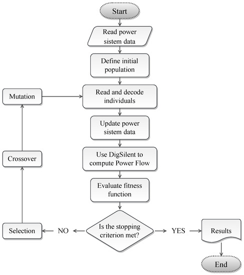
Figure 4. Flowchart of the implemented GA.

In the first stage of the algorithm, an initial population of randomly or pseudo-randomly candidate solutions is generated. Every candidate solution is represented as a vector (chromosome) that contains the four optimization variables of the system as indicated in Figure 5.

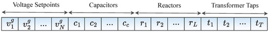
Figure 5. Illustration of a candidate solution to the ORPD problem.

In this case, the initial population is randomly created taking into account the limits of the optimization variables. Once the initial population is obtained, the quality or fitness of every individual is computed. This corresponds to the power losses given by Equation (1). For this, a power flow is executed for every candidate solution using DIgSILENT and taking as inputs the information provided in their codification.

The next step of the GA is the process of selection. In this step, two subsets of the population are randomly selected, and the fittest individual from each subset is chosen to generate new candidate solutions (offspring). The two selected individuals or candidate solutions are then the parents of new solutions that are obtained through a crossover operation. In this stage, the information of the parents is exchanged at a random position. The last stage of the GA is the mutation in which a randomly selected element of the chromosome is changed. This steps allows the algorithm to escape from locally-optimal solutions.

Within the GA, the size of the population is kept constant; therefore, new solutions or offspring replace the worst solutions of the current population. The process is carried out until a given number of generations is executed.

3.4.2. MVMO

The MVMO is a population-based stochastic technique which performs a search procedure within a normalized range of optimization variables. The MVMO uses the same structure of candidate solutions as illustrated in Figure 6. MVMO uses the solution variables as an adaptive memory to save the n-best solutions that are found, a generic version available in [59]. Like other evolutionary solution algorithms, MVMO adopts an optimal value criterion to select the main solution, i.e., the stored optimal solution, from which the next generation (offspring) solution is created.

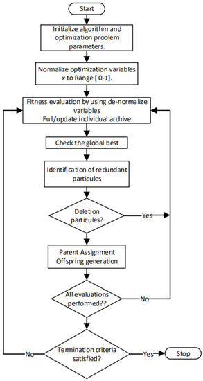
Figure 6. Flowchart of the implemented MVMO algorithm.

The search space of the MVMO for all variables is limited to [0, 1]. So then, the maximum and minimum values of the variables must be normalized in this range. In each iteration, it is not possible that any solution component surpasses the corresponding constraints. To achieve this goal, a unique mapping function ($h-$function) was developed. This function has as inputs the means and variance of the best candidate solutions that the optimization algorithm has found so far. The shape and mapping curves are fixed in relation to the advancement in the search space, and the MVMO updates the good solution around the best solutions in each iteration [60]. The MVMO algorithm searches around the best local candidate solution with a small possibility of being trapped in a local optimal solution. The feasibility of the solution is examined, and a fitness value is given for this solution. To handle constraints, the static penalization approach was implemented. In this case, all variables are restricted by applying the fitness function due to the fact that control variables are self-limited.

The mapping function is in charge of transforming a given variable $x_i^{*}$ varied randomly with unity distribution to another variable $x_i$, which is concentrated around the mean value.

The solutions file is the knowledge base of the methodology that guides the search. Then, the n best solutions or individuals found so far by the MVMO are stored in this file. The fitness value of each solution is also saved. The update is only performed if the new solution candidate turns out to be better than those currently in the file. The viable solutions are at the top of the file. These individuals are sorted in accordance to their fitness value. Non-viable solutions are sorted in accordance to their fitness and are placed at the bottom of the file. Once the file is complete with n feasible individuals, any non-feasible candidate solutions will not have a chance to be saved in the file.

The best solution found so far (the first solution positioned in the file), labeled as xbest, is the parent. In this case, a variable selection is carried out for the generation of the offspring. The MVMO algorithm seeks the mean value stored in the solution file for the best individual only in m selected directions. Therefore, only these dimensions of the offspring are updated, while the remaining $D-m$ are assigned the corresponding $xbest$ values, D being the number of control variables (problem dimension). Next, the mutation stage is carried out for each selected m dimension.

The MVMO also has a swarm variant with $n_p$ particles. In this case, each particle has its own solution file and mapping function. In the swarm MVMO algorithm, every particle carries out m steps to identify an optimal set of independent solutions. Subsequently, the current solutions (particles) exchange information. In some cases, some solution candidates might be very close to each other, meaning that there is information redundancy, and therefore, redundant particles must be discarded. The best local and global solution ($gbest$) are defined. In addition, the normalized distance between each solution to the best local and global solutions are calculated.

The ith particle is eliminated from the process if its normalized distance is lower than a certain predefined threshold; if the solution is still considered, its search is focused towards the global best solution. This is performed by assigning the global best solution as the parent. Finally, the MVMO search process stops after a given number of fitness evaluations. The authors in [61,62] present a detailed description of the swarm MVMO algorithm.

4. Description of the Test Systems

The main features and data of the power systems under study are presented in this section for future validation of the proposed approach. These systems have 6, 14 and 39 buses, respectively. The last two systems can be found directly in the DIgSILENT software [31].

4.1. IEEE 6-Bus Test System

Figure 7 depicts the IEEE 6-bus test system used in this study. The system features two power generators located at buses 2 and 6 (slack bus), 2 capacitive banks, 2 power transformers and 5 transmission lines. Table 1 presents the data of these devices which include the nominal parameters of capacitor banks, transformers, generators and loads. In this case, the capacitor banks were represented as synchronous compensators featuring nominal capabilities from 0 to 5 MVAr.

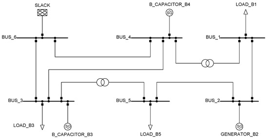
Figure 7. IEEE 6-bus test system diagram.

Table 1. Electrical data of the IEEE 6-bus test system.

Transmission Lines
Line	From	To	Line Impedance’s
#	Bus	Bus	R ($\mathsf{\Omega }$)	X ($\mathsf{\Omega }$)
1	6	3	4.88187	20.55942
2	6	4	3.17520	14.68530
3	4	3	3.84993	16.15383
4	5	2	11.19258	25.40160
5	2	1	28.69587	41.67450
Transformer Characteristics
Transformer	From	To	Transformer Tap
#	Bus	Bus	Settings
1	4	1	9100
2	3	5	9100
Bus-Bar Characteristics
Bus	Load		Power Injections
#	${\mathit{P}}_{\mathit{L}}$(MW)	${\mathit{Q}}_{\mathit{L}}$(Mvar)	${\mathit{P}}_{\mathit{G}}$(MW)	${\mathit{Q}}_{\mathit{G}}$(Mvar)
1	55	13	0	0
2	0	0	50	0
3	50	5	0	5
4	0	0	0	5
5	30	18	0	0
6	-	-	Slack node

Table 2 presents the transformer data of this system. In this case, the maximum range for a safe operation of these transformers is of $\pm 10\%$. The data presented in Table 2 are needed for the parametrization of transformers in DIgSILENT.

Table 2. Characterization of transformers in the IEEE 6-bus test system.

Transformer	From	To	Minimum	Maximum	Addition Voltage	Voltage
#	Bus	Bus	Voltage	Voltage	per Tap (%)	Range (%)
1	4	1	9100	11,100	0.001	−0.1 $\le$pT$\le$ 0.1
2	3	5	9100	11,100	0.001	−0.1 $\le$pT$\le$ 0.1

Note that the last column in Table 2 defines the parameter pT to define the percentage of variations of the voltage output in the transformers equipped with taps. It is worth mentioning that the minimum and maximum positions for the transformer’s taps (see columns 4 and 5 in Table 2 are related with the typical settings in DIgSILENT software where the nominal input/output voltages for the transformer are defined for a tap value of 10,000.

Table 3 presents the technical characteristics of the generators present in the IEEE 6-bus test system. In this case, bus 2 is a voltage-controlled node with minimum and maximum voltages of $0.95$ p.u. and $1.15$ p.u., respectively. On the other hand, bus 6 is assigned as the slack or reference bus. For comparative purposes with [31], its minimum and maximum voltages are assigned as $0.95$ p.u. and $1.15$ p.u., respectively.

Table 3. Technical characteristics of the generators in the IEEE 6-bus test system.

Generator	Terminal	${\mathit{v}}_1^{\mathit{g},min}={\mathit{v}}_6^{\mathit{g},min}$(p.u.)	${\mathit{v}}_1^{\mathit{g},max}$ (p.u.)	${\mathit{v}}_6^{\mathit{g},max}$ (p.u.)
1	2	0.95	1.1	1.15
Slack	6	0.95	1.05	1.1

4.2. IEEE 14-Bus Test System

The IEEE 14-bus test system is illustrated in Figure 8. This system includes 5 transformers, 16 transmission lines, 2 generators and 3 capacitor banks. This power system is also made of four areas with voltage levels of 132 kV, 33 kV, 11 kV and 1 kV.

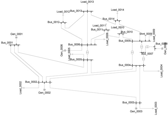
Figure 8. IEEE 14-bus test system diagram.

Table 4 presents the electrical parameter of the transmission lines for the IEEE 14-bus test system, while Table 5 shows the transformers information. In this system the slack node is bus 1, and node 2 is a voltage-controlled bus. Furthermore, three synchronous compensators are used as capacitor banks operating in the continuous domain. These elements are located at buses 3, 6 and 8; buses 3 and 6 feature a nominal power of 20 MVAr and bus 8 a nominal power of 30 MVAr.

Table 4. Parameters for the IEEE 14-bus test system.

Transmission Lines
Line	From	To	Line Impedance’s		Line	From	To	Line Impedance’s
#	Bus	Bus	R ($\mathsf{\Omega }$)	X ($\mathsf{\Omega }$)	#	Bus	Bus	R ($\mathsf{\Omega }$)	X ($\mathsf{\Omega }$)
1	1	2	6.753542	20.61956	9	6	11	1.034332	2.16602
2	1	2	6.753542	20.61956	10	6	12	1.33849	2.78577
3	1	5	9.414187	38.86250	11	6	13	0.72037	1.41864
4	2	3	8.187537	34.49428	12	9	10	0.34641	0.92020
5	2	4	10.12509	30.72200	13	9	14	1.38422	2.94443
6	2	5	9.922968	30.29685	14	10	11	0.89352	2.09164
7	3	4	11.67582	29.80027	15	12	13	2.40581	2.17669
8	4	5	2.326104	7.33724	16	13	14	1.86142	3.78993
Transformers Characteristic
Trans.	From	To	Tap		Trans.	From	To	Tap
#	Bus	Bus	Settings		#	Bus	Bus	Settings
1	5	6	11,100		4	8	7	11,100
2	4	9	11,100		5	4	7	11,100
3	9	7	11,100
Bus-Bar Characteristics (All Power Units inMW and MVAr)
Bus	Load		Injection		Bus	Load		Injection
#	${\mathit{P}}_{\mathit{L}}$	${\mathit{Q}}_{\mathit{L}}$	${\mathit{P}}_{\mathit{G}}$	${\mathit{Q}}_{\mathit{G}}$	#	${\mathit{P}}_{\mathit{L}}$	${\mathit{Q}}_{\mathit{L}}$	${\mathit{P}}_{\mathit{G}}$	${\mathit{Q}}_{\mathit{G}}$
1	-	-	Node Slack		8	0.0	0.0	0.0	30.0
2	21.7	12.7	40.0	42.4	9	29.5	16.6	0.0	0.0
3	94.2	19.0	0.0	20.0	10	9.0	5.8	0.0	0.0
4	47.8	−3.9	0.0	0.0	11	3.5	1.8	0.0	0.0
5	7.6	1.6	0.0	0.0	12	6.1	1.6	0.0	0.0
6	11.2	7.5	0.0	20.0	13	13.5	5.8	0.0	0.0
7	0.0	0.0	0.0	20.0	14	14.9	5.0	0.0	0.0

Table 5. Transformers characteristics of the IEEE 14-bus test system.

Transformer	From	To	Minimum	Maximum	Addition Voltage	Voltage
#	Bus	Bus	Voltage	Voltage	per Tap (%)	Range (%)
1	4	7	9100	11,100	0.0022	−2.2 $\le$pT$\le$ 2.2
2	4	9	9100	11,100	0.0031	−3.1 $\le$pT$\le$ 3.1
3	5	6	9100	11,100	0.0068	−6.8 $\le$pT$\le$ 6.8
4	8	7	9100	11,100	0.0068	−6.8 $\le$pT$\le$ 6.8
5	9	7	9100	11,100	0.0068	−6.8 $\le$pT$\le$ 6.8

4.3. IEEE 39-Bus Test System

The IEEE 39-bus test system, illustrated in Figure 9, features four areas with voltage levels of 345 kV, 230 kV, 138 kV and 16.5 kV. This system has 10 generators, 34 transmission lines and 12 transformers.

Figure 9. IEEE 39-bus test system diagram.

The electrical parameters of the IEEE 39-bus test system and the characterization of the transformers are indicated in Table 6 and Table 7, respectively.

Table 6. Parameters of the IEEE 39-bus test system.

Lines Characteristic
Line	From	To	Line Impedance’s		Line	From	To	Line Impedance’s
#	Bus	Bus	R ($\mathsf{\Omega }$)	X ($\mathsf{\Omega }$)	#	Bus	Bus	R ($\mathsf{\Omega }$)	X ($\mathsf{\Omega }$)
1	1	2	0.025547	0.30	18	13	14	0.026732	0.30
2	1	39	0.012000	0.30	19	14	15	0.024884	0.30
3	2	3	0.025827	0.30	20	15	16	0.028723	0.30
4	2	25	0.244186	0.30	21	16	17	0.023595	0.30
5	3	4	0.018309	0.30	22	16	19	0.024615	0.30
6	3	18	0.024812	0.30	23	16	21	0.017777	0.30
7	4	5	0.018750	0.30	24	16	24	0.015254	0.30
8	4	14	0.018604	0.30	25	17	18	0.025609	0.30
9	5	6	0.023076	0.30	26	17	27	0.022543	0.30
10	5	8	0.021428	0.30	27	21	22	0.017142	0.30
11	6	7	0.019565	0.30	28	22	23	0.018750	0.30
12	6	11	0.025609	0.30	29	23	24	0.018857	0.30
13	7	8	0.026086	0.30	30	25	26	0.029721	0.30
14	8	9	0.019008	0.30	31	26	27	0.028571	0.30
15	9	39	0.012000	0.30	32	26	28	0.027215	0.30
16	10	11	0.027906	0.30	33	26	29	0.027360	0.30
17	10	13	0.027906	0.30	34	28	29	0.027814	0.30
Transformers Characteristic
Trans.	From	To	Tap		Trans.	From	To	Tap
#	Bus	Bus	Settings		#	Bus	Bus	Settings
1	2	30	9100		7	19	33	9100
2	6	31	9100		8	20	34	9100
3	10	32	9100		9	22	35	9100
4	11	12	9100		10	23	36	9100
5	13	12	9100		11	25	37	9100
6	19	20	9100		12	29	38	9100
Bus Characteristics (All Power Units in MW and MVAr)
Bus	Load		Injection		Bus	Load		Injection
#	${\mathit{P}}_{\mathit{L}}$	${\mathit{Q}}_{\mathit{L}}$	${\mathit{P}}_{\mathit{G}}$	${\mathit{P}}_{\mathit{G}}$	#	${\mathit{P}}_{\mathit{L}}$	${\mathit{Q}}_{\mathit{L}}$	${\mathit{P}}_{\mathit{G}}$	${\mathit{P}}_{\mathit{G}}$
3	322.0	2.4	-	-	27	281.0	75.5	-	-
4	500.0	184.0	-	-	28	206.0	27.6	-	-
7	233.8	84.0	-	-	29	283.5	26.9	-	-
8	522.0	176.0	-	-	30	-	-	250	0.0
12	7.5	88.0	-	-	31	9.2	4.6	Slack bus
15	320.0	153.0	-	-	32	-	-	650	0.0
16	329.0	32.3	-	-	33	-	-	632	0.0
18	158.0	30.0	-	-	34	-	-	254	0.0
20	628.0	103.0	-	-	35	-	-	650	0.0
21	274.0	115	-	-	36	-	-	560	0.0
23	247.5	84.6	-	-	37	-	-	540	0.0
24	308.0	−92.2	-	-	38	-	-	830	0.0
25	224.0	47.2	-	-	39	1104	250	1000	0.0
26	139.0	17.0	-	-

Table 7. Characterization of the transformers in the IEEE 39-bus test system.

Transformer	From	To	Minimum	Maximum	Addition Voltage	Voltage
#	Bus	Bus	Voltage	Voltage	per Tap (%)	Range (%)
1	02	30	9100	11,100	0.0025	−2.5 $\le$pT$\le$ 2.5
2	25	37	9100	11,100	0.0025	−2.5 $\le$pT$\le$ 2.5
3	29	38	9100	11,100	0.0025	−2.5 $\le$pT$\le$ 2.5
4	22	35	9100	11,100	0.0025	−2.5 $\le$pT$\le$ 2.5
5	23	36	9100	11,100	0.0070	−7.0 $\le$pT$\le$ 7.0
6	19	33	9100	11,100	0.0070	−7.0 $\le$pT$\le$ 7.0
7	20	34	9100	11,100	0.0009	−0.9 $\le$pT$\le$ 0.9
8	19	20	9100	11,100	0.0060	−6.0 $\le$pT$\le$ 6.0
9	10	32	9100	11,100	0.0070	−7.0 $\le$pT$\le$ 7.0
10	13	12	9100	11,100	0.0006	−0.6 $\le$pT$\le$ 0.6
11	11	12	9100	11,100	0.0006	−0.6 $\le$pT$\le$ 0.6
12	06	31	9100	11,100	0.0070	−7.0 $\le$pT$\le$ 7.0

5. Tests and Results

This section presents the results obtained with the power systems described in Section 4. All tests were run on a personal computer Intel(R) Core(TM) i5-8365U processor 1.60 GHz. RAM 16 Gb, with a Windows 10 operating system, 64 bits, single language. The results of the two implemented methodologies (MVMO and GA) using the Python-DIgSILENT interface described in this paper are compared with those obtained through the CBGA proposed in [31] using DPL. For the sake of simplicity, only Case A1 of the aforementioned paper is considered.

5.1. Results with the IEEE 6-Bus Test System

Table 8 presents the results obtained with the developed Python-DIgSILENT interface considering MVMO and GA. These results are compared with the CBGA implemented in [31].

Table 8. Results for the IEEE 6-bus test system.

Elements	Base Case	CBGA [31]	MVMO	GA
Generators	Voltage (p.u.)	Voltage (p.u.)
G1 Bus06 (slack)	1.0000	1.0500	1.0500	1.0500
G2 Bus02	1.0000	1.0999	1.0999	1.0999
Transformers	Tap Position	Tap Position
Trafo Bus 04-01	9100	11,089	11,100	11,099
Trafo Bus 03-05	9100	11,099	11,085	11,099
Capacitor Bank	Reactive power (Mvar)	Reactive power (Mvar)
PQ Bus03	0.0000	4.9992	4.9999	4.9999
PQ Bus04	0.0000	4.9995	4.9999	4.9999
Power Losses (MW)	12.910	10.089	10.089	10.089
Reduction (%)	-	21.85	21.85	21.85

The results presented in Table 8 show that the reduction in power losses obtained with the three algorithms is identical and corresponds to 21.85% with respect to the original values (base case). Note that the voltage set points of the generators obtained with the three optimization approaches is also the same. In this case the voltage set point for the slack bus is 1.05 p.u., and the maximum voltage magnitude for generation buses is 1.1 p.u. The capacitor banks installed in the test system operate almost at their maximum limits in the three approaches explored. Regarding tap positions of transformers, there are some small differences between the results obtained with proposed interface (both MVMO and GA) and the DIgSILENT DPL (CBGA); nonetheless, such difference does not alter the amount of power loss reduction.

Table 9 presents the line loading. It can be observed that the three optimization methods result in roughly the same loading conditions. In all cases, it is reduced, resulting in lower power losses. Some transmission lines reduce their loading conditions by an important percentage: for example, line 6-3 that passes from an initial condition of 48.23% to 41.26% or line 6-4 that passes from 55.8% to 47.4% .

Table 9. Line loading for the IEEE 6-bus test system considering different approaches.

Line	Base Case	CBGA [31]	MVMO	GA
(Start-End)	Loading (%)	Loading (%)	Loading (%)	Loading (%)
Line 6-3	48.2314	41.2668	41.2645	41.2661
Line 6-4	55.8039	47.4526	47.4497	47.4517
Line 4-3	10.9207	9.5843	9.5841	9.5842
Line 5-2	33.5334	30.4007	30.4016	30.4008
Line 1-2	17.4563	16.1338	16.1339	16.1337

Figure 10 illustrates the voltage magnitudes for each simulation along with the base case. Note that for all methodologies, there is an important enhancement of the voltage profile: nonetheless, without violating the voltage limits of the system. Note that some buses exhibit important voltage improvements, such as bus 2 that passes from 1.00 p.u. to 1.10 p.u. and bus 3 that originally has 0.84 p.u. and passes to 0.94 p.u.

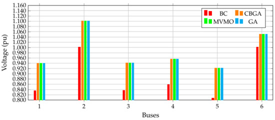
Figure 10. Voltage profile of the IEEE 6-bus test system considering different methodologies.

5.2. Results with the IEEE 14-Bus Test System

Table 10 presents the optimal reactive power outputs in capacitor banks, voltage set points of generators, tap positions of transformers and the total power losses for each methodology compared to the base case. The active power loss reduction is around 21% for the three methodologies. The highest reduction is obtained with the CBGA; nonetheless, the differences with the other two methodologies implemented in the proposed Python-DIgSILENT interface are not high. In this case, the solution obtained with the CBGA is 0.1% and 0.4% better than those achieved with MVMO and GA, respectively. The voltage set point for the slack bus is kept the same for the three methodologies; nonetheless, there are small differences in the voltage set points obtained for the PV bus. The CBGA proposes 1.037 p.u for generator G2 located at bus 02, while MVMO and GA set this voltage at 1.0353 p.u. and 1.03723 p.u., respectively. Regarding tap position, all methodologies coincide in the same results. Note that unlike the IEEE 6-bus test system, where transformer taps were set close to their maximum values, in this test system the results of the taps were different. Such variation in transformer tap positions are principally conditioned by voltage output in power generators. On the other hand, capacitor banks with nominal rates of 20 MVAr for the compensators located at nodes PQBus06 and PQBus08 and 30 MVAr for the capacitor at bus PQB03 present small differences with the three methodologies. Note that this last one is not set near its upper limit as is the case for the other capacitor banks.

Table 10. Results for the IEEE 14-bus test system.

Elements	Base Case	CBGA [31]	MVMO	GA
Generators	Voltage (p.u.)		Voltage (p.u.)
G1 Bus01(slack)	1.0000	1.0500	1.0500	1.0500
G2 Bus02	1.0000	1.0370	1.0353	1.03723
Transformers	Tap Position		Tap Position
Trafo Bus 05-06	11,100	9100	9100	9100
Trafo Bus 04-09	11,100	9100	9100	9100
Trafo Bus 09-07	11,100	11,100	11,100	11,000
Trafo Bus 08-07	11,000	9100	9100	9100
Trafo Bus 04-07	11,000	9100	9100	9100
Capacitor Bank	Reactive power (Mvar)		Reactive power (Mvar)
PQ Bus06	0.0000	19.9936	19.9996	19.9997
PQ Bus08	0.0000	19.9902	19.9998	19.9998
PQ Bus03	0.0000	26.4670	26.2454	19.9999
Power Losses (MW)	17.200	13.558	13.560	13.573
Reduction (%)	-	21.18	21.16	21.08

The line loading for the base case and for each implemented metaheuristic is presented in Table 11. In this case, results after optimization are roughly the same for the three methodologies. Note that there is a reduction in the power flows in all lines. In particular, Line 1–10 passes from a loading of 12.48% to 6.1%. In addition, lines 9–10 and 9–14 experience high loading, passing from 28.54% and 28.99% to approximately 13.8% and 17.4%, respectively, after optimization.

Table 11. Loading conditions of lines for the IEEE 14-bus test system.

Line	Original Values	CBGA [31]	MVMO	GA
(Start-End)	Loading (%)	Loading (%)	Loading (%)	Loading (%)
Line 1–2(1)	36.7486	32.9993	33.0110	33.0158
Line 1–2(2)	36.7486	32.9993	33.0110	33.0158
Line 1–5	33.3443	31.6365	31.6361	31.6289
Line 2–3	35.2074	30.8695	30.8654	30.8590
Line 2–4	27.7888	23.7087	23.7032	23.7258
Line 2–5	21.1140	17.5080	17.5030	17.5326
Line 3–4	11.3021	10.4849	10.4861	10.4167
Line 4–5	30.5788	27.1440	27.1426	27.1161
Line 6–11	13.1368	11.6951	11.6912	11.7381
Line 6–12	15.4418	12.7432	12.7398	12.7746
Line 6–13	34.6838	29.6405	29.6321	29.7191
Line 9–10	28.5486	13.8137	13.8158	13.7414
Line 9–14	28.9935	17.4872	17.4853	17.4782
Line 10–11	12.4895	6.1880	6.1879	6.1764
Line 12–13	2.3032	2.5620	2.5609	2.5750
Line 13–14	9.9979	8.8853	8.8826	8.9126

Figure 11 illustrates the voltage profile of the IEEE 14-bus test system for the base case and every optimization technique. Note that an important improvement on voltage profile is achieved through the optimization techniques without violating the lower and upper voltage bounds of the system.

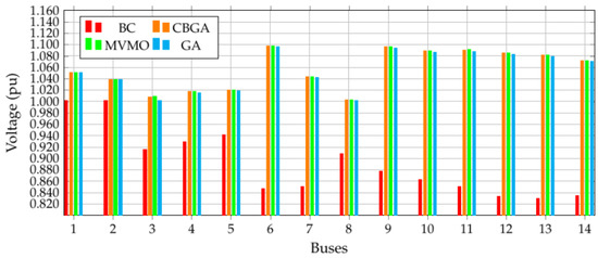
Figure 11. Voltage profile of the IEEE 14-bus system considering different methodologies.

It can be seen in Figure 11 that some buses show important improvement in their voltage magnitudes, such as buses 10 to 14 which start with a relatively low voltage around 0.85 p.u. and end up with nearly 1.1 p.u. after the optimization process. This change is mainly due to the new positions of transformer taps and the reactive power injected by the capacitor banks.

5.3. Results with the IEEE 39-Bus Test System

The solutions obtained with the IEEE 39-bus test system are reported in Table 12. These include voltage set points of generators and transformer tap positions (this test system does not feature capacitor banks). In this case, the solution achieved by the MVMO matches the one obtained by the CBGA (although with different values of the optimization variables). On the other hand, the reduction obtained by the GA implemented in the Python-DIgSILENT interface is slightly better than that of the CBGA and MVMO. Nonetheless, the three methodologies achieve a reduction of power losses of around 31% with respect to the base case. An important feature of these three solutions is the variability of the optimization variables which evidences the multimodal feature of the ORPD.

Table 12. Results for the IEEE 39-bus system.

Elements	Base Case	CBGA [31]	MVMO	GA
Generators	Voltage (p.u)		Voltage (p.u)
G1 Bus39	1.0000	1.0776	1.0657	1.0753
G2 Bus31(slack)	1.0000	1.0500	1.0500	1.0500
G3 Bus32	1.0000	1.0810	1.0728	1.0903
G4 Bus33	1.0000	1.0985	1.0733	1.0917
G5 Bus34	1.0000	1.0414	1.0764	1.0995
G6 Bus35	1.0000	1.0970	1.0879	1.0891
G7 Bus36	1.0000	1.0761	1.0574	1.0857
G8 Bus37	1.0000	1.0792	1.0703	1.0960
G9 Bus38	1.0000	1.0982	1.0841	1.0880
G10 Bus30	1.0000	1.0652	1.0565	1.0725
Transformers	Tap Position		Tap Position
Trafo Bus 02-30	9100	10,440	10,863	10,416
Trafo Bus 25-37	9100	10,830	11,100	11,100
Trafo Bus 29-38	9100	10,021	11,100	10,844
Trafo Bus 22-35	9100	10,214	9455	9480
Trafo Bus 23-36	9100	11,065	9397	10,850
Trafo Bus 19-33	9100	10,562	10,169	10,892
Trafo Bus 20-34	9100	9648	10,966	10,222
Trafo Bus 19-20	9100	10,729	9,335	10,041
Trafo Bus 10-32	9100	11,037	11,100	10,927
Trafo Bus 13-12	9100	10,725	11,100	10,737
Trafo Bus 11-12	9100	10,085	10,971	10,373
Trafo Bus 06-31	9100	11,058	10,635	10,179
Power Losses (MW)	38.790	26.476	26.479	26.422
Reduction(%)	-	31.75	31.75	31.88

The loading percentage of each transmission line obtained with the three optimization methodologies is presented in Table 13. As with the previous test systems, a generalized reduction in loading conditions is experienced in all lines. It is worth mentioning that the power flow relief in transmission lines for this system is higher than that of the previous test systems. In fact, most transmission lines have an important loading reduction with the exception of lines 1–39 and 14–15 that experience a small increment in their power flows.

Table 13. Loading conditions of the lines for the IEEE 39-bus system.

(Lines (Start-End)	Base Case Loading	CBGA [31] (%)	MVMO Loading	GA (%)
L 1–2	31.5919	21.9571	20.7607	21.2570
L 1–2	31.5919	21.9571	20.7607	21.2570
L 1–39	24.6876	24.1132	25.7837	25.0039
L 2–3	71.5882	56.8398	56.8912	56.7258
L 2–25	44.4287	37.9134	38.0674	37.8657
L 3–4	30.8098	16.9084	17.1695	17.4032
L 3–18	13.0756	9.0992	9.6112	8.8264
L 4–5	27.6425	22.7757	22.5411	22.5985
L 4–14	50.5295	43.9437	44.0914	43.7494
L 5–6	86.2751	72.2391	72.5483	72.1871
L 5–8	59.1632	50.8941	51.3915	50.9805
L 6–7	79.2231	67.6418	68.1481	67.7006
L 6–11	67.1245	58.4637	58.3799	58.2336
L 7–8	35.6682	29.4048	29.7223	29.4501
L 8–9	37.8915	12.2439	9.8735	11.5506
L 9–39	32.0210	17.0125	19.1821	17.6749
L 10–11	67.6012	59.4466	59.5977	58.8809
L 10–13	54.5243	46.9344	46.3916	46.8317
L 13–14	52.3392	44.1616	43.9891	43.8117
L 13–14	52.3392	44.1616	43.9891	43.8117
L 14–15	5.2454	8.0803	7.0235	7.5485
L 15–16	62.7392	51.7655	52.1361	51.9074
L 16–17	46.8878	35.5673	35.4393	35.5494
L 16–19	92.5581	77.7325	77.6822	77.6428
L 16–21	60.7955	51.6157	51.2743	51.3467
L 16–24	17.5808	17.7158	17.3047	17.2731
L 17–18	38.4347	32.6810	32.9077	32.5544
L 17–27	13.8078	6.2314	6.1114	5.7034
L 21–22	112.7630	93.7010	93.8989	93.7535
L 22–23	22.7600	11.7429	7.1108	7.2783
L 23–24	64.0312	54.1063	53.9617	53.9557
L 25–26	16.4244	12.6808	13.3907	11.8264
L 26–27	51.4229	41.5517	41.6268	41.3364
L 26–28	25.3862	23.5066	23.3028	23.9918
L 26–29	33.9377	31.4868	31.2730	31.9884
L 28–29	60.7682	53.7901	53.6518	54.1180

The voltage profile of the IEEE 39-bus test system is illustrated in Figure 12 for the base case and for the solutions obtained with the implemented methodologies. Note that there is an important improvement in voltage profile; nonetheless, these remain within their bounds. This implies that the proposed tested methodologies ensure the feasibility of the proposed solutions.

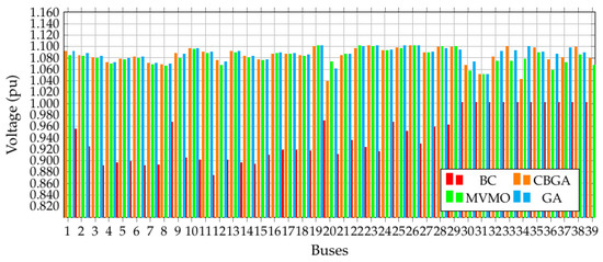
Figure 12. Voltage profile of the IEEE 39-bus test system considering different methodologies.

5.4. Processing Times

The average processing times required by the proposed Python-DIgSILENT interface and the CBGA implemented in the DPL environment from DIgSILENT [31] are presented in Table 14. As expected, processing times increase with the number of nodes since more decision variables must be considered in the optimization processes. Note that an important improvement in computation time is achieved through the proposed approach, especially when applying the GA.

Table 14. Average processing times for all the IEEE test systems considering different optimization approaches.

Test System	CBGA [31] (s)	MVMO (s)	GA (s)
IEEE 6-bus test system	88.94	24.47	14.45
IEEE 14-bus test system	124.74	43.96	29.96
IEEE 39-bus test system	193.80	132.59	89.42

6. Conclusions

This paper presented a Python-DIgSILENT interface to approach the optimal reactive power dispatch problem in electric power systems. The proposed interface takes advantage of all the functionalities provided by DIgSILENT software for system modeling and power flow calculations along with an object-oriented high-level programming language that allows using optimization libraries. The optimal reactive power dispatch was solved using two metaheuristic approaches, namely MVMO and GA. Several tests were carried out on three benchmark IEEE power systems. Voltage set points of generators, transformer tap positions and reactive power injection in capacitor banks were used as optimization variables.

The numerical results reported power loss reductions with respect to the base case of up to 21.85%, 21.1% and 31.88% for the IEEE-6, 14 and 39 bus test systems, respectively. This evidenced the effectiveness of the proposed approach for reducing active power losses through the optimal management of reactive power resources. All tests were carried out with a fixed voltage of the slack bus of 1.05 p.u and a maximum voltage in generation buses of 1.1 p.u. In all cases, it was verified that voltage magnitudes were kept within their allowable limits. On the other hand, significant reductions on loading conditions were observed in all test systems.

A comparison was carried out with previously reported results in the specialized literature. The proposed approach was able to match the results obtained by a CBGA implemented in DIgSILENT programming language using the same test systems and initial conditions. Nonetheless, better computing times were obtained with the proposed approach.

The proposed Python-DIgSILENT interface opens the possibility to explore other metaheuristic methodologies available in Python optimization libraries. Future work may also include other variants of the optimal reactive power dispatch, such as considering a multi-period and multi-area approach as well as taking into account voltage stability issues.

References

- Villa-Acevedo, W.M.; López-Lezama, J.M.; Valencia-Velásquez, J.A. A Novel Constraint Handling Approach for the Optimal Reactive Power Dispatch Problem. Energies 2018, 11, 2352. [Google Scholar] [CrossRef]
- Marín-Cano, C.C.; Sierra-Aguilar, J.E.; López-Lezama, J.M.; Jaramillo-Duque, Á.; Villegas, J.G. A Novel Strategy to Reduce Computational Burden of the Stochastic Security Constrained Unit Commitment Problem. Energies 2020, 13, 3777. [Google Scholar] [CrossRef]
- Sierra-Aguilar, J.E.; Marín-Cano, C.C.; López-Lezama, J.M.; Jaramillo-Duque, Á.; Villegas, J.G. A New Affinely Adjustable Robust Model for Security Constrained Unit Commitment under Uncertainty. Appl. Sci. 2021, 11, 3987. [Google Scholar] [CrossRef]
- Mota-Palomino, R.; Quintana, V.H. Sparse Reactive Power Scheduling by a Penalty Function - Linear Programming Technique. IEEE Trans. Power Syst. 1986, 1, 31–39. [Google Scholar] [CrossRef]
- Quintana, V.; Santos-Nieto, M. Reactive-power dispatch by successive quadratic programming. IEEE D 1989, 4, 425–435. [Google Scholar] [CrossRef]
- Granville, S. Optimal reactive dispatch through interior point methods. IEEE Trans. Power Syst. 1994, 9, 136–146. [Google Scholar] [CrossRef]
- López-Lezama, J.M.; Cortina-Gómez, J.; Muñoz-Galeano, N. Assessment of the Electric Grid Interdiction Problem using a nonlinear modeling approach. Electr. Power Syst. Res. 2017, 144, 243–254. [Google Scholar] [CrossRef]
- Gracia-Velásquez, D.G.; Morales-Rodríguez, A.S.; Montoya, O.D. Application of the Crow Search Algorithm to the Problem of the Parametric Estimation in Transformers Considering Voltage and Current Measures. Computers 2022, 11, 9. [Google Scholar] [CrossRef]
- Arenas-Acuña, C.A.; Rodriguez-Contreras, J.A.; Montoya, O.D.; Rivas-Trujillo, E. Black-Hole Optimization Applied to the Parametric Estimation in Distribution Transformers Considering Voltage and Current Measures. Computers 2021, 10, 124. [Google Scholar] [CrossRef]
- Saldarriaga-Zuluaga, S.D.; López-Lezama, J.M.; Muñoz-Galeano, N. Optimal coordination of over-current relays in microgrids considering multiple characteristic curves. Alex. Eng. J. 2021, 60, 2093–2113. [Google Scholar] [CrossRef]
- Pareja, L.A.G.; Lezama, J.M.L.; Carmona, O.G. Optimal Placement of Capacitors, Voltage Regulators, and Distributed Generators in Electric Power Distribution Systems. Ingeniería 2020, 25, 334–354. [Google Scholar] [CrossRef]
- Montoya, O.D. Notes on the Dimension of the Solution Space in Typical Electrical Engineering Optimization Problems. Ingeniería 2022, 27, e19310. [Google Scholar] [CrossRef]
- Duman, S.; Sonmez, Y.; Guvencc, U.; Yorukeren, N. Optimal reactive power dispatch using a gravitational search algorithm. IET Gener. Transm. Distrib. 2012, 6, 563. [Google Scholar] [CrossRef]
- Shaw, B.; Mukherjee, V.; Ghoshal, S. Solution of reactive power dispatch of power systems by an opposition-based gravitational search algorithm. Int. J. Electr. Power Energy Syst. 2014, 55, 29–40. [Google Scholar] [CrossRef]
- Khazali, A.; Kalantar, M. Optimal reactive power dispatch based on harmony search algorithm. Int. J. Electr. Power Energy Syst. 2011, 33, 684–692. [Google Scholar] [CrossRef]
- Yoshida, H.; Kawata, K.; Fukuyama, Y.; Takayama, S.; Nakanishi, Y. A particle swarm optimization for reactive power and voltage control considering voltage security assessment. IEEE Trans. Power Syst. 2000, 15, 1232–1239. [Google Scholar] [CrossRef]
- Cai, G.; Ren, Z.; Yu, T. Optimal Reactive Power Dispatch Based on Modified Particle Swarm Optimization Considering Voltage Stability. In Proceedings of the 2007 IEEE Power Engineering Society General Meeting, Tampa, FL, USA, 24–28 June 2007; pp. 1–5. [Google Scholar] [CrossRef]
- Vlachogiannis, J.; Lee, K. A Comparative Study on Particle Swarm Optimization for Optimal Steady-State Performance of Power Systems. IEEE Trans. Power Syst. 2006, 21, 1718–1728. [Google Scholar] [CrossRef]
- Gutiérrez, D.; Villa, W.M.; López-Lezama, J.M. Flujo Óptimo Reactivo mediante Optimización por Enjambre de Partículas. Inform. Tecnol. 2017, 28, 215–224. [Google Scholar] [CrossRef][Green Version]
- Naderi, E.; Narimani, H.; Fathi, M.; Narimani, M.R. A novel fuzzy adaptive configuration of particle swarm optimization to solve large-scale optimal reactive power dispatch. Appl. Soft Comput. 2017, 53, 441–456. [Google Scholar] [CrossRef]
- Duong, T.L.; Duong, M.Q.; Phan, V.D.; Nguyen, T.T. Optimal Reactive Power Flow for Large-Scale Power Systems Using an Effective Metaheuristic Algorithm. J. Electr. Comput. Eng. 2020, 2020, 1–11. [Google Scholar] [CrossRef]
- Londoño, D.C.; Villa-Acevedo, W.M.; López-Lezama, J.M. Assessment of Metaheuristic Techniques Applied to the Optimal Reactive Power Dispatch. In Communications in Computer and Information Science; Springer International Publishing: Cham, Switzerland, 2019; pp. 250–262. [Google Scholar] [CrossRef]
- Saddique, M.S.; Bhatti, A.R.; Haroon, S.S.; Sattar, M.K.; Amin, S.; Sajjad, I.A.; ul Haq, S.S.; Awan, A.B.; Rasheed, N. Solution to optimal reactive power dispatch in transmission system using meta-heuristic techniques—Status and technological review. Electr. Power Syst. Res. 2020, 178, 106031. [Google Scholar] [CrossRef]
- Zhao, J.; Zhang, Z.; Yao, J.; Yang, S.; Wang, K. A distributed optimal reactive power flow for global transmission and distribution network. Int. J. Electr. Power Energy Syst. 2019, 104, 524–536. [Google Scholar] [CrossRef]
- Khan, N.H.; Wang, Y.; Tian, D.; Raja, M.A.Z.; Jamal, R.; Muhammad, Y. Design of Fractional Particle Swarm Optimization Gravitational Search Algorithm for Optimal Reactive Power Dispatch Problems. IEEE Access 2020, 8, 146785–146806. [Google Scholar] [CrossRef]
- Jamal, R.; Men, B.; Khan, N.H.; Raja, M.A.Z.; Muhammad, Y. Application of Shannon Entropy Implementation Into a Novel Fractional Particle Swarm Optimization Gravitational Search Algorithm (FPSOGSA) for Optimal Reactive Power Dispatch Problem. IEEE Access 2021, 9, 2715–2733. [Google Scholar] [CrossRef]
- Vlachogiannis, J.G.; Lee, K.Y. Quantum-Inspired Evolutionary Algorithm for Real and Reactive Power Dispatch. IEEE Trans. Power Syst. 2008, 23, 1627–1636. [Google Scholar] [CrossRef]
- Ela, A.A.E.; Abido, M.; Spea, S. Differential evolution algorithm for optimal reactive power dispatch. Electr. Power Syst. Res. 2011, 81, 458–464. [Google Scholar] [CrossRef]
- Bakirtzis, A.; Biskas, P.; Zoumas, C.; Petridis, V. Optimal power flow by enhanced genetic algorithm. IEEE Trans. Power Syst. 2002, 17, 229–236. [Google Scholar] [CrossRef]
- Ara, A.L.; Kazemi, A.; Gahramani, S.; Behshad, M. Optimal reactive power flow using multi-objective mathematical programming. Sci. Iran. 2012, 19, 1829–1836. [Google Scholar] [CrossRef]
- Bernal-Romero, D.L.; Montoya, O.D.; Arias-Londoño, A. Solution of the Optimal Reactive Power Flow Problem Using a Discrete-Continuous CBGA Implemented in the DigSILENT Programming Language. Computers 2021, 10, 151. [Google Scholar] [CrossRef]
- Ganesh, S.; Perilla, A.; Torres, J.R.; Palensky, P.; van der Meijden, M. Validation of EMT Digital Twin Models for Dynamic Voltage Performance Assessment of 66 kV Offshore Transmission Network. Appl. Sci. 2020, 11, 244. [Google Scholar] [CrossRef]
- Mei, R.N.S.; Sulaiman, M.H.; Mustaffa, Z.; Daniyal, H. Optimal reactive power dispatch solution by loss minimization using moth-flame optimization technique. Appl. Soft Comput. 2017, 59, 210–222. [Google Scholar] [CrossRef]
- Bhongade, S.; Tomar, A.; Goigowal, S.R. Minimization of Optimal Reactive Power Dispatch Problem using BAT Algorithm. In Proceedings of the 2020 IEEE First International Conference on Smart Technologies for Power, Energy and Control (STPEC), Nagpur, India, 25–26 September 2020; IEEE: Piscataway, NJ, USA, 2020. [Google Scholar] [CrossRef]
- Abido, M.A. Optimal Power Flow Using Tabu Search Algorithm. Electr. Power Compon. Syst. 2002, 30, 469–483. [Google Scholar] [CrossRef]
- Lenin, K. Reduction of active power loss by improved tabu search algorithm. Int. J. Res. GRANTHAALAYAH 2018, 6, 1–9. [Google Scholar] [CrossRef]
- ElSayed, S.K.; Elattar, E.E. Slime Mold Algorithm for Optimal Reactive Power Dispatch Combining with Renewable Energy Sources. Sustainability 2021, 13, 5831. [Google Scholar] [CrossRef]
- Rojas, D.G.; Lezama, J.L.; Villa, W. Metaheuristic Techniques Applied to the Optimal Reactive Power Dispatch: A Review. IEEE Lat. Am. Trans. 2016, 14, 2253–2263. [Google Scholar] [CrossRef]
- Aghbolaghi, A.J.; Tabatabaei, N.M.; Boushehri, N.S.; Parast, F.H. Reactive Power Optimization in AC Power Systems. In Power Systems; Springer International Publishing: Cham, Switzerland, 2017; pp. 345–409. [Google Scholar] [CrossRef]
- Barboza, L.V.; Ziirn, H.H.; Salgado, R. Load Tap Change Transformers: A Modeling Reminder. IEEE Power Eng. Rev. 2001, 21, 51–52. [Google Scholar] [CrossRef]
- Londoño-Tamayo, D.; Villa-Acevedo, J.L.L.W. Mean-Variance Mapping Optimization Algorithm Applied to the Optimal Reactive Power Dispatch. INGECUC 2021, 17, 239–255. [Google Scholar] [CrossRef]
- Sharif, S.; Taylor, J. MINLP formulation of optimal reactive power flow. In Proceedings of the IEEE 1997 American Control Conference (Cat. No.97CH36041), Albuquerque, NM, USA, 8–10 May 1997. [Google Scholar] [CrossRef]
- Morán-Burgos, J.A.; Sierra-Aguilar, J.E.; Villa-Acevedo, W.M.; López-Lezama, J.M. A Multi-Period Optimal Reactive Power Dispatch Approach Considering Multiple Operative Goals. Appl. Sci. 2021, 11, 8535. [Google Scholar] [CrossRef]
- Acosta, M.N.; Adiyabazar, C.; Gonzalez-Longatt, F.; Andrade, M.A.; Torres, J.R.; Vazquez, E.; Santos, J.M.R. Optimal Under-Frequency Load Shedding Setting at Altai-Uliastai Regional Power System, Mongolia. Energies 2020, 13, 5390. [Google Scholar] [CrossRef]
- Gonzalez-Longatt, F.M.; Rueda, J.L. (Eds.) PowerFactory Applications for Power System Analysis; Springer International Publishing: Cham, Switzerland, 2014. [Google Scholar] [CrossRef]
- Bifaretti, S.; Bonaiuto, V.; Pipolo, S.; Terlizzi, C.; Zanchetta, P.; Gallinelli, F.; Alessandroni, S. Power Flow Management by Active Nodes: A Case Study in Real Operating Conditions. Energies 2021, 14, 4519. [Google Scholar] [CrossRef]
- Dierbach, C. Python as a First Programming Language. J. Comput. Sci. Coll. 2014, 29, 73. [Google Scholar]
- Thurner, L.; Scheidler, A.; Schäfer, F.; Menke, J.H.; Dollichon, J.; Meier, F.; Meinecke, S.; Braun, M. Pandapower—An Open-Source Python Tool for Convenient Modeling, Analysis, and Optimization of Electric Power Systems. IEEE Trans. Power Syst. 2018, 33, 6510–6521. [Google Scholar] [CrossRef]
- Milano, F. A python-based software tool for power system analysis. In Proceedings of the 2013 IEEE Power Energy Society General Meeting, Vancouver, BC, Canada, 21–25 July 2013; pp. 1–5. [Google Scholar] [CrossRef]
- Condren, J.; An, S. Automation of transmission planning analysis process using Python and GTK+. In Proceedings of the 2006 IEEE Power Engineering Society General Meeting, London, UK, 18–22 June 2006; p. 8. [Google Scholar] [CrossRef]
- Yusuff, A.; Mosetlhe, T.; Ayodele, T. Statistical method for identification of weak nodes in power system based on voltage magnitude deviation. Electr. Power Syst. Res. 2021, 200, 107464. [Google Scholar] [CrossRef]
- Latif, A.; Ahmad, I.; Palensky, P.; Gawlik, W. Multi-objective reactive power dispatch in distribution networks using modified bat algorithm. In Proceedings of the 2016 IEEE Green Energy and Systems Conference (IGSEC), Long Beach, CA, USA, 6–7 June 2016; pp. 1–7. [Google Scholar] [CrossRef]
- Mean Variance Mapping Optimization Algorithm. Available online: https://pypi.org/project/MVMO/ (accessed on 30 April 2022).
- Pymoo: Multi-Objective Optimization in Python. Available online: https://pymoo.org/index.html (accessed on 30 April 2022).
- Blank, J.; Deb, K. Pymoo: Multi-Objective Optimization in Python. IEEE Access 2020, 8, 89497–89509. [Google Scholar] [CrossRef]
- Implemtación de MVMO y GA en DigSilent Power Factory con Python. Available online: https://github.com/Msanchez1002/MVMO_GA (accessed on 30 April 2022).
- Agudelo, L.; López-Lezama, J.M.; Muñoz-Galeano, N. Vulnerability assessment of power systems to intentional attacks using a specialized genetic algorithm. Dyna 2015, 82, 78–84. [Google Scholar] [CrossRef]
- GA: Genetic Algorithm. Available online: https://pymoo.org/algorithms/soo/ga.html (accessed on 30 April 2022).
- MVMo: Mean Variance Mapping Optimization Algorithm. Available online: https://github.com/dgusain1/MVMO (accessed on 30 April 2022).
- Erlich, I.; Venayagamoorthy, G.K.; Worawat, N. A Mean-Variance Optimization algorithm. In Proceedings of the IEEE Congress on Evolutionary Computation, Barcelona, Spain, 18–23 July 2010; pp. 1–6. [Google Scholar] [CrossRef]
- Rueda, J.L.; Erlich, I. Optimal dispatch of reactive power sources by using MVMO optimization. In Proceedings of the 2013 IEEE Computational Intelligence Applications in Smart Grid (CIASG), Singapore, 16–19 April 2013; pp. 29–36. [Google Scholar] [CrossRef]
- Rueda, J.L.; Erlich, I. Evaluation of the mean-variance mapping optimization for solving multimodal problems. In Proceedings of the 2013 IEEE Symposium on Swarm Intelligence (SIS), Singapore, 16–19 April 2013; pp. 7–14. [Google Scholar] [CrossRef]
Publisher’s Note: MDPI stays neutral with regard to jurisdictional claims in published maps and institutional affiliations. |
© 2022 by the authors. Licensee MDPI, Basel, Switzerland. This article is an open access article distributed under the terms and conditions of the Creative Commons Attribution (CC BY) license (https://creativecommons.org/licenses/by/4.0/).